Peripheral arterial disease screening for hemodialysis patients using a fractional‐order integrator and transition probability decision‐making model

Abstract

Atherosclerosis and resultant peripheral arterial disease (PAD) are common complications in patients with type 2 diabetes mellitus or end‐stage renal disease and in elderly patients. The prevalence of PAD is higher in patients receiving haemodialysis therapy. For early assessment of arterial occlusion using bilateral photoplethysmography (PPG), such as changes in pulse transit time and pulse shape, bilateral timing differences could be used to identify the risk level of PAD. Hence, the authors propose a discrete fractional‐order integrator to calculate the bilateral area under the systolic peak (AUSP). These indices indicated the differences in both rise‐timing and amplitudes of PPG signals. The dexter and sinister AUSP ratios were preliminarily used to separate the normal condition from low/high risk of PAD. Then, transition probability‐based decision‐making model was employed to evaluate the risk levels. The joint probability could be specified as a critical threshold, < 0.81, to identify the true positive for screening low or high risk level of PAD, referring to the patients’ health records. In contrast to the bilateral timing differences and traditional methods, the proposed model showed better efficiency in PAD assessments and provided a promising strategy to be implemented in an embedded system.

1. Introduction

Cardiovascular diseases (CVDs), involving heart or vascular diseases, are major risk factors for morbidity and mortality especially in elderly patients and haemodialysis (HD) patients with or without type 2 diabetes. In Taiwan, the prevalence of CVDs in elderly patients aged > 65 years is associated with several complications, such as coronary artery disease, stroke, hypertensive heart disease, peripheral arterial disease (PAD), and venous thrombosis. Compared to other complications, PAD and atherosclerotic diseases are common and occur in both lower and upper extremity peripheral arteries [1, 2]. Endothelial dysfunction in vascular access has been found to be a contributing cause of atherosclerosis due to diabetes mellitus. Therefore, patients develop atherosclerosis of peripheral arteries, peripheral vascular stenosis, and subsequent vascular diseases [3, 4]. Lower limb PAD is highly prevalent in patients with type 2 diabetes mellitus. This symptom leads to narrowed lower extremity peripheral arteries, leg pain, and/or foot gangrene [5, 6, 7]. In addition, patients with peritoneal dialysis and HD therapy also develop PAD in both lower and upper limbs. Frequent complications, such as venous side stenosis or stenoses near the graft‐to‐vein site, could reduce dialysis blood flow [8, 9, 10]. In this study, we propose a prognostic detection model that could be employed to screen PAD with bilateral photoplethysmography (PPG) signals in HD patients.

PPG signals carry physical information about cardiovascular functions, heart rates, arterial properties, and arterial/venous blood oxygen saturation in clinical examinations [7, 11, 12, 13, 14, 15, 16]. Optical measurement techniques (red and infrared wavelengths) allow for comfortable and non‐invasive continuous monitoring of biosignals and the placement of reflection or transmissive modes on any skin surface. Thus, optical probes and measurement hardware could be easily integrated into a mobile device or a tablet PC via wired or wireless communication, as shown in Fig. 1. Using bilateral multisite measurements or temporal analysis, previous studies [7, 11, 12, 13, 17, 18, 19] have shown significant bilateral PPG differences, such as timing differences and PPG morphology, in CVDs, PAD, arterial compliance, diabetic foot, and vascular diseases. An advantage of optical measurements is their ability to detect changes in vasoconstriction and vasodilatation in vessels < 2.5 mm in diameter. Information about blood volume and blood transport can be obtained via continuous measurement and temporal analysis at different body sites.

Fig. 1.

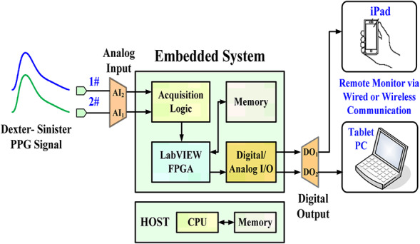
Configuration of proposed screening model in an embedded system

Time‐domain methods are commonly applied to analyse PPG signals for lower and upper limb PAD screening. Bilateral differences in rise time (RT), pulse transit time (PTT), and pulse waveforms have been validated that could separate normal condition from lower grade or higher grade PAD. Depending on the severity of PAD progression, the dexter‐to‐sinister dissimilarity in transit time and pulse amplitudes increases significantly. Thus, pulse area under the systolic peak (AUSP) contains both information. This index has been validated so as to identify patients with and without PAD [15, 17, 18]. A quantitative method based on discrete fractional‐order integrators [7, 20, 21] with finite computations, short‐memory requirements, and finite power series was designed to calculate the bilateral pulse AUSPs. This method could overcome the limitations of Fourier analysis and wavelet transformation methods, such as the large number of numerical computations, memory and sampling data requirements, and choices of specific frequency features for healthy subjects and PAD subjects [12, 22]. The Markov model [23, 24] with two states of AUSP ratios expresses a matrix of substitution rates [24, 25, 26] to replace the bilateral AUSP variations. Bilateral differences in transition probabilities have been employed to separate normal conditions from low‐risk/high‐risk PAD using the distance estimation method. The joint probability was specified as a critical threshold to find the similarity or different states for screening bilateral AUSP variations. These quantities were inversely related to the severity of PAD and were then employed to identify the possible levels. This method could overcome the complex computations and was easy to program into an embedded system.

The remaining of this paper is organised as follows: Section 2 describes the PPG measurement, feature choice, and screening, such as timing parameters, pulse shape indices, and AUSPs; Section 3 addresses the methodology of the study, including the discrete fractional‐order integrator and transition probability model; and Sections 4 and 5 present the experimental results and conclusions.

2. PPG measurement, features, and screening

PPG is a non‐invasive optical measurement and a volumetric measurement that provides an estimation of blood variations, pulse volumes, and blood transport via the measurement of dynamic attenuation of red or infrared light. With light from a light‐emitting source, a photodetector/photosensor monitors the changes in light absorption using the reflection or transmissive mode to convert light signals into voltage signals. The detector can be placed, either bilaterally or unilaterally, at different body sites, such as the earlobes, index fingers, thumbs, big toes, and on the forehead [11, 12, 13, 14, 15], as shown in the transmissive absorption mode in Fig. 2. The PPG pulse is attributable to variations in blood volume in the skin surface, caused by the heart pumps, cardiovascular regulation, thermoregulation, respiration, and pressure pulses. Hence, the heart rate, cardiac cycle, and respiration can be detected.

Fig. 2.

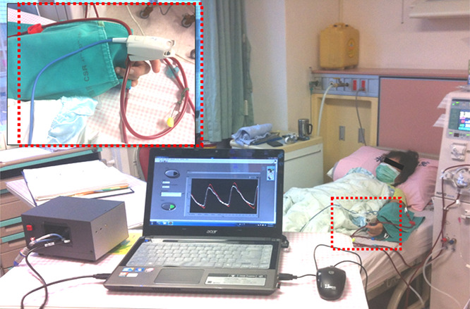
PPG optical measurements at the thumbs

A PPG waveform consists of alternating current (ac) and direct current (dc) components that carry human physiological information. The amplitudes of PPG ac components are proportional to the pressure pulses, while the differences between the systolic and diastolic pressure will result in the blood changes in the peripheral arteries. The PPG's systolic peak is a result of pressure wave from the left ventricle to the periphery of the human body. Hence, the systolic region of each PPG pulse is a time interval revealing vascular dynamic compliances, as shown by the RT of normalised PPG waveform in Fig. 3. Thus, PPG can be used to evaluate cardiovascular risk factors, atherosclerosis, arterial properties, endothelial function, and hypertension [11, 12, 13, 14, 15]. Some indices, such as the reflection index, augmentation index, and stiffness index, have been used to evaluate arterial stiffness, arterial compliance, and vascular health. These indexes are estimated depending on the systolic peak, diastolic peak, and dicrotic notch duration [17, 18]. However, age‐related change is an important factor that could affect the pulse shape characteristics, such as degradation of arterial compliance with age or increase of arterial stiffness with age [15]. The dicrotic notch and diastolic peak may disappear or be less pronounced in older and unhealthy subjects. These indexes cannot be used for subjects of all ages. Timing parameters, such as RT (foot‐to‐systolic peak time) and PTT (R‐peak to systolic peak time) [11, 12, 13], where the peak of R wave of electrocardiogram is a timing reference, show that for bilateral differences (dexter‐to‐sinister), ΔRT = |RT _R − RT _L | and ΔPTT = |PTT _R − PTT _L |, as vascular disease gradually evolves; this is highly correlated with the evaluation of vascular diseases and peripheral arterial stenoses for subjects of all ages. However, timing parameters in signal processing need an extra R peak detection from an electrocardiogram as a timing reference.

Fig. 3.

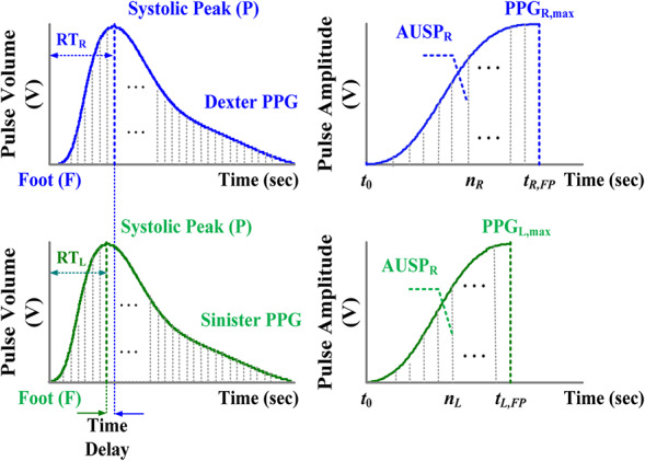
Bilateral normalised PPG signals and bilateral AUSPs

In this study, the AUSP is used to evaluate the bilateral differences from the pulse foot (F) to the systolic peak (P) in the time‐domain PPG signal, as shown in Fig. 3. The characteristics of systolic region show a similar correlation for subjects with different ages. It can be seen the AUSP has an obvious characteristic feature involving timing (time delay) and amplitude information and can be used as a non‐invasive continuous measurement. This index increases with age and systolic stress, while systolic load increases due to arterial stiffness and vascular compliance degradations. The risk factors of CVD, diabetes, and PAD have an important consequence to identify vascular disease progression. Hence, the dexter‐to‐sinister AUSP ratio, ρ, is used to evaluate bilateral similarity and difference, and the critical rule is defined as follows:

$$\rho =\frac{\text{AUS}{\mathrm{P}}_R}{\text{AUS}{\mathrm{P}}_L}=\left\{\begin{array}{c}>1_{,}\text{AUS}{\mathrm{P}}_R>\text{AUS}{\mathrm{P}}_L\\ \begin{array}{c}\simeq 1_{,}\text{AUS}{\mathrm{P}}_R\simeq \text{AUS}{\mathrm{P}}_L\\ <1_{,}\text{AUS}{\mathrm{P}}_R<\text{AUS}{\mathrm{P}}_L\end{array}\end{array}\right.$$ (1)

where AUSP ratio > 1 or < 1 represents bilateral differences in PAD screening.

3. Methodology

3.1. Discrete fractional‐order integrator

For integral computations, fractional‐order integrator employs non‐integer numbers to output the time integral of its input signals, such as electrical signals, audio signals, and biosignals. The summation processes are computed using the ratios of the gamma function, Γ(α), which incorporates the number of sampling data points in the time interval [t ₀, t ₁], the fractional order parameters, α [21]. For information and signal processing, temporal analysis of a time‐varying signal, f(t), is performed in discrete time steps using the Grünwald–Letnikov (G–L) definition [20, 21], as follows:

$$D^{-\alpha }f(t)\simeq \underset{\mathrm{\Delta }\tau \to 0}{\lim }(\mathrm{\Delta }\tau ){}^{\alpha }\sum _{i=0}^{n-1}\left|{(-1)}^i\left(\begin{array}{c}-\alpha \\ i\end{array}\right)f(t-i\times \mathrm{\Delta }\tau )\right|$$ (2)

where 0 < α < 1 for integral process, α∈R; −1 < α < 0 for derivative process; integer, α= ± 1, for integer‐order differentiation and integration process; n is the number of sampling points; and the binomial coefficients are given as follows:

$$\begin{array}{rl}\left(\begin{array}{c}\alpha \\ 0\end{array}\right)& =1,\left(\begin{array}{c}-\alpha \\ i\end{array}\right)=\frac{-\alpha (-\alpha -1)\cdots (-\alpha -i+1)}{i!}\\ & =\frac{\mathrm{\Gamma }(-\alpha -1)}{\mathrm{\Gamma }(i+1)\mathrm{\Gamma }(-\alpha -i+1)}\end{array}$$ (3)

Traditional differentiation and integration computations use the integer‐order differential operators with Tustin transforms and trapezoidal integration methods for geometrical interpretations. The G–L integrator employs non‐integer and irrational numbers to deal with signals, and the summation is computed using the ratios of the gamma function, Γ(α), and sampling data, f(t–i·Δt), in the time interval [t ₀, t ₁]. It can be used to express the finite power series or series expansion of non‐linear functions as a weighted summation to approximate the integral. Its integrator with the various parameters, α, has a broad application range for the analysis of time‐varying signals which includes fluid flows, heat conduction, and biosignals.

For bilateral PPG signals, the AUSP is calculated and bounded in the specific time interval [t ₀, t _FP] using the discrete fractional‐order integration, as shown in Fig. 3. Hence, the AUSP of dexter‐PPG and sinister‐PPG is defined as

$$\text{AUS}{\mathrm{P}}_R\simeq \underset{\mathrm{\Delta }{\tau }_R\to 0}{\lim }(\mathrm{\Delta }{\tau }_R){}^{\alpha }\sum _{i=0}^{n_R-1}\left|{(-1)}^i\left(\begin{array}{c}-\alpha \\ i\end{array}\right)\text{PP}{\mathrm{G}}_{R,\text{FP}}[i\times \mathrm{\Delta }{\tau }_R]\right|$$ (4)

$$\text{AUS}{\mathrm{P}}_L\simeq \underset{\mathrm{\Delta }{\tau }_L\to 0}{\lim }(\mathrm{\Delta }{\tau }_L){}^{\alpha }\sum _{j=0}^{n_L-1}\left|{(-1)}^j\left(\begin{array}{c}-\alpha \\ j\end{array}\right)\text{PP}{\mathrm{G}}_{L,\text{FP}}[j\times \mathrm{\Delta }{\tau }_L]\right|$$ (5)

timing step:

$$\mathrm{\Delta }{\tau }_R=\left(\frac{t_{R,\text{FP}}-t_0}{n_R}\right)\in R\text{and}\mathrm{\Delta }{\tau }_L=\left(\frac{t_{L,\text{FP}}-t_0}{n_L}\right)\in R$$ (6)

where the discrete dexter‐PPG signal is referred to as PPG _{R ,FP}[i × Δτ_R ] in time interval [t ₀, t_{R ,FP}], the number of sampling points, i∈[0, n_R −1]; the discrete sinister‐PPG signal is referred to as PPG _{L ,FP}[j × Δτ_L ] in time interval [t ₀, t_{L ,FP}], the number of sampling points, j∈[0, n_L −1]; n_R and n_L are integer numbers. Both the AUSP _R and AUSP _L are functions of the variable fractional order, 0 < α < 1, and they have a broad range for feature extraction of time‐varying PPG signals. In addition, the discrete bilateral PPG signals can be normalised as follows:

$$\text{PP}{\mathrm{G}}_{R,\text{PF}}[i\times \mathrm{\Delta }{\tau }_R]=\frac{\text{PP}{\mathrm{G}}_R[i\times \mathrm{\Delta }{\tau }_R]}{\text{PP}{\mathrm{G}}_{R,\max }},i\in \left[0,n_R-1\right]$$ (7)

$$\text{PP}{\mathrm{G}}_{L,\text{PF}}[j\times \mathrm{\Delta }{\tau }_L]=\frac{\text{PP}{\mathrm{G}}_L[j\times \mathrm{\Delta }{\tau }_L]}{\text{PP}{\mathrm{G}}_{L,\max }},j\in \left[0,n_L-1\right]$$ (8)

where PPG _{R ,max} and PPG _{L ,max} are the systolic peaks of bilateral PPG signals, and the initial conditions are PPG _R [0] = PPG _L [0] = 0, as shown in Fig. 3.

3.2. Transition probability model

The bilateral AUSP ratios, ρ_R and ρ_L , are defined as follows:

$${\rho }_R=\frac{\text{AUS}{\mathrm{P}}_R}{\text{AUS}{\mathrm{P}}_L}\text{and}{\rho }_L=\frac{\text{AUS}{\mathrm{P}}_L}{\text{AUS}{\mathrm{P}}_R}$$ (9)

The AUSP ratios are used to evaluate bilateral similarity, as the ratios, > 1 or < 1, represent bilateral differences in peripheral arterial stenosis screening. Therefore, each pair of AUSP ratios, ρ_R and ρ_L , can be replaced by the substitution rates, such as the parameters, λ ₁ and λ ₂. For two states, the concept of substitution‐rate matrix, Q , is defined as follows [24, 26]:

$$\begin{array}{rl}\mathit{Q}& =\left[\begin{array}{cc}{\rho }_{11}& {\rho }_{12}\\ {\rho }_{21}& {\rho }_{22}\end{array}\right]\\ & =\left[\begin{array}{cc}-{\rho }_R& {\rho }_R\\ {\rho }_L& -{\rho }_L\end{array}\right]=\mathit{U}\mathbf{\Lambda }{\mathit{U}}^{-1},{\rho }_{12}=-{\rho }_{11},{\rho }_{21}=-{\rho }_{22}\end{array}$$ (10)

$$\Rightarrow \mathit{Q}=\mathit{U}\mathbf{\Lambda }{\mathit{U}}^{-1}=\left[\begin{array}{cc}{u}_{11}& u_{12}\\ u_{21}& u_{22}\end{array}\right]\left[\begin{array}{cc}{\lambda }_1& 0\\ 0& {\lambda }_2\end{array}\right]{\left[\begin{array}{cc}{u}_{11}& u_{12}\\ u_{21}& u_{22}\end{array}\right]}^{-1}$$ (11)

where each raw element of the matrix, Q , sums to 0 (−ρ_R  + ρ_R  = 0 and ρ_L −ρ_L  = 0); matrix, U , is a non‐singular matrix and U ⁻¹ is its inverse; Λ is a diagonal matrix, diag{λ ₁, λ ₂}; and λ ₁ and λ ₂ are the eigenvalues of matrix Q .

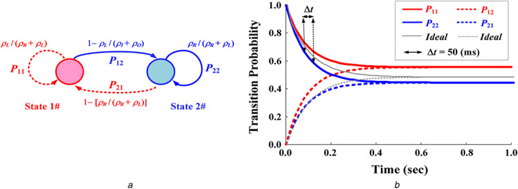
For two dynamic states, λ ₁ × Δt or λ ₂ × Δt gives the probabilities that the ratio ‘ρ_R will change to ρ_L ’ or ‘ρ_L will change to ρ_R ’ in an infinitely small time interval, Δt. A transition matrix can be used to describe the dynamics of changes in two ratios, while two observations can be classified. This provides a Markov transition probability model to describe the evolution of the change ratings, as shown in Fig. 4a . The transition probability matrix, P _RL (t) = [p_rl ]_2×2, is defined as follows:

$${\mathit{P}}_{RL}(t)=e^{Qt}=\left[\begin{array}{cc}{p}_{11}(t)& p_{12}(t)\\ p_{21}(t)& p_{22}(t)\end{array}\right]=\left[\begin{array}{cc}{p}_{11}(t)& (1-p_{11}(t))\\ (1-p_{22}(t))& p_{22}(t)\end{array}\right]$$ (12)

subject to $0\le p_{rl}(t)\le 1$, ${\sum }_{l=1}^2{p}_{rl}(t)=1$, r = 1, 2; l = 1, 2. The spectral decomposition of substitution‐rate matrix, Q , is also [24]

$$\mathit{Q}=U\mathrm{\Lambda }{U}^{-1}=\left[\begin{array}{cc}1& -{\rho }_R\\ 1& {\rho }_L\end{array}\right]\left[\begin{array}{cc}0& 0\\ 0& -\mathrm{\Delta }\end{array}\right]\left[\begin{array}{cc}\frac{{\rho }_R}{\mathrm{\Delta }}& \frac{{\rho }_L}{\mathrm{\Delta }}\\ \frac{-1}{\mathrm{\Delta }}& \frac{1}{\mathrm{\Delta }}\end{array}\right]$$ (13)

where Δ = (ρ_R  + ρ_L ). After deriving the transition probability matrix, P (t), for Markov chain with two dynamic states, the general formulation is

$$P_{RL}(t)=e^{Qt}=U\left[\begin{array}{cc}{e}^{0\times t}& 0\\ 0& e^{-\mathrm{\Delta }\times t}\end{array}\right]U^{-1}$$ (14)

$$\begin{array}{rl}\Rightarrow P_{RL}(t)& =\left[\begin{array}{cc}{P}_{11}(t)& P_{12}(t)\\ P{}_{21}(t)& P_{22}(t)\end{array}\right]\\ & =\frac{1}{({\rho }_R+{\rho }_L)}\cdot \left[\begin{array}{cc}{\rho }_L+{\rho }_R{e}^{-({\rho }_R+{\rho }_L)t}& {\rho }_R-{\rho }_R{e}^{-({\rho }_R+{\rho }_L)t}\\ {\rho }_L-{\rho }_L{e}^{-({\rho }_R+{\rho }_L)t}& {\rho }_R+{\rho }_L{e}^{-({\rho }_R+{\rho }_L)t}\end{array}\right]\end{array}$$ (15)

Fig. 4.

Transition probability model

(a) Markov chain with two states, (b) Transition probabilities for bilateral asynchronous screening (average t_RL  = 1.0 s, N = 20, Δt = 50 ms)

When time t increases from 0 to ∞ (t→∞), the stationary limiting distributions are

$$\underset{t\to \mathrm{\infty }}{\lim }{P}_{11}(t)=\underset{t\to \mathrm{\infty }}{\lim }{P}_{21}(t)=\frac{{\rho }_L}{({\rho }_R+{\rho }_L)}$$ (16)

$$\underset{t\to \mathrm{\infty }}{\lim }{P}_{22}(t)=\underset{t\to \mathrm{\infty }}{\lim }{P}_{12}(t)=\frac{{\rho }_R}{({\rho }_R+{\rho }_L)}$$ (17)

If ρ_R  1.0 and ρ_L  ; 1.0, the transition probabilities will approach the limiting distribution, [0.5, 0.5, 0.5, and 0.5], over any time, t ≥ 0, as shown by the ideal transition probabilities in Fig. 4. Hence, the ideal transition probability is

$$\begin{array}{rl}\Rightarrow P_{\text{ideal}}(t)& =\left[\begin{array}{cc}{P}_{11,\text{ideal}}& P_{12,\text{ideal}}\\ P_{21,\text{ideal}}& P_{22,\text{ideal}}\end{array}\right]\\ & =\left[\begin{array}{cc}0.5e^{-2t}+0.5& -0.5e^{-2t}+0.5\\ -0.5e^{-2t}+0.5& 0.5e^{-2t}+0.5\end{array}\right]\end{array}$$ (18)

We can then apply a column vector [P ₁₁(t) P ₂₂(t)]^T to estimate sequence similarity with the pair of AUSP ratios, ρ_R and ρ_L . The Euclidean distance estimation is used to screen the similarity, as follows [26]:

$$d_R=\sqrt{\sum _{n=1}^N{(P_{11}(n)-P_{11,\text{ideal}}(n))}^2}$$ (19)

$$d_L=\sqrt{\sum _{n=1}^N{(P_{22}(n)-P_{22,\text{ideal}}(n))}^2}$$ (20)

where N is the number of sampling points within infinitely small time intervals, Δt = t_RL /N, n = 1, 2, 3,…, N. In time interval t_RL , the joint probability accommodating the variance with AUSP ratios, ρ_R and ρ_L , is as follows:

$$\begin{array}{rl}{p}_{RL}(t_{RL})& =p_R(t_{RL})\times p_L(t_{RL})\\ & =\exp \left(-\frac{1}{2}{\left(\frac{d_R}{\sigma }\right)}^2\right)\times \exp \left(-\frac{1}{2}{\left(\frac{d_L}{\sigma }\right)}^2\right)\end{array}$$ (21)

where σ is the standard deviation; $p_R(t_{RL})>0.90$ and $p_L(t_{RL})>0.90$ are used to separate the normal condition from PAD progression.

As shown in (21), p_R (t_RL ) and p_L (t_RL ) are used to screen the same ratio of each pair of dexter‐to‐sinister AUSPs. The Euclidean distance estimation screens the bilateral differences due to the asymmetric AUSP. When two ratios are different, the limitation values of transition probabilities will diverge from 0.50 with time intervals over 1.0 s, as shown in Fig. 4b . Thus, the joint probability, p_RL , gradually decreases and approaches zero. Its quantity, from value 1.00 to value 0.00, would be inversely related to PAD progression.

3.3. Model implementation in an embedded system

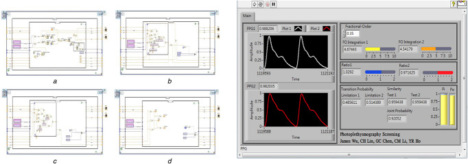
A field programmable gate array (FPGA) is a high‐level embedded system that can be designed to perform the specific functions, as an application‐specific integrated circuit (ASIC) to implement the given application. The detection method integrating the discrete fractional‐order integrator and the transition probability model was configured in an embedded system (NI^TM, myRio 1900, FPGA module [27]). The integrating algorithm was designed in a LabView FPGA module using the ‘Timed Loop’ and the ‘Stacked Sequence Structure’. The logics of data acquisition, fractional‐order integrators, and transition probability model were implemented in each stacked sequence structure, as shown in Fig. 5. Data acquisition logic performed the PPG signal preprocessing to obtain the sampling data of dexter and sinister AUSPs in the (a) sequence structure. Two logics of fractional‐order integrators were carried out using the arithmetic and gamma function operations in the (b) and (c) sequence structures. Then, the dexter and sinister fractional‐order AUSPs can be achieved to calculate the AUSP ratios. While timed loop was used since be deterministic loop, it would synchronise to the internal clock of the embedded system. Both two‐sequence structures finished the calculations before each time period was achieved. With the timed loop, the implemented loop rate for the arithmetic operations was 40 MHz (25 ns for each loop). Hence, two fractional‐order AUSP calculations took about n_R  × 25 ns and n_L  × 25 ns execution time. As indicated in (16) and (17), the transition probability model was implemented in (d) sequence structure. The final output of joint probability exceeding value 0.81 (p_R (t_RL ) > 0.90 and p_L (t_RL ) > 0.90) separated normal conditions from a PAD progression. The inference results could simulate and verify the logic designs via the graphic user interface, as shown in Fig. 5. Among the current designs, the graphic user interface for Windows application has reprogrammability and flexibility to quickly debug and develop ASICs. Thus, the high‐level FPGA module provided a promising platform to design a prototype monitor for bilateral PPG screening. The overall detection procedure is shown in Fig. 6.

Fig. 5.

Sequence structures and graphic user interface for PPG signal processing and arithmetic operations

(a) Data acquisition logic, (b) , (c) Logic of fractional‐order integrator, (d) Logic of transition probability model

Fig. 6.

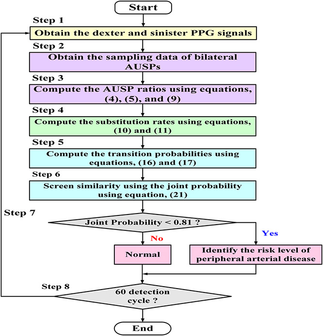
Flowchart of detection procedure

4. Experimental results and discussion

4.1. Feasibility tests with the proposed screening model

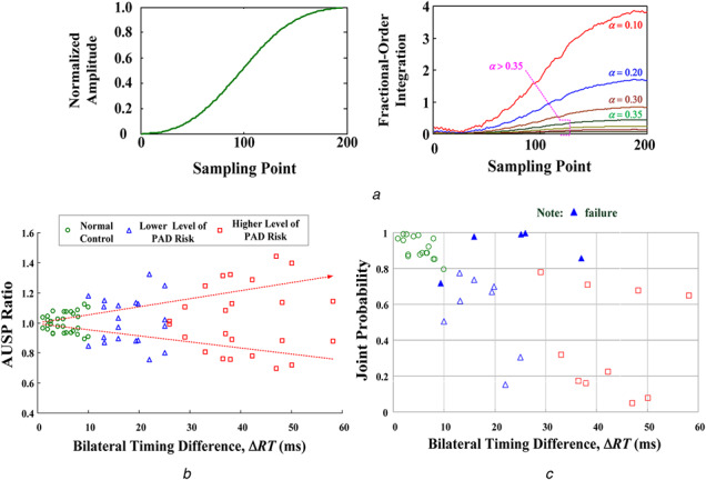
This experiment was approved by the Human Research Ethics Committee and the Institutional Review Board (IRB) of Hospital (under contract number: VGHKS13‐CT12‐11). A total of 40 enrolled subjects were divided into normal subjects (18 subjects) and subjects with PADs, CVDs, or diabetes mellitus (22 subjects) and were further divided into three groups: (i) normal condition, (ii) lower level of PAD risk, and (iii) higher level of PAD risk. Two thumb clips with mounted light‐emitting diodes and photodetectors were placed on the dexter and sinister thumbs to obtain bilateral PPG signals using the transmissive absorption mode, as shown in Fig. 2. Thereby, two‐channel temporal PPG analysis was performed using a data acquisition controller from the photosensors to a tablet PC. Then, the measurement data were stored in the memory. The prototype detection method, which involves data acquisition, discrete fractional‐order integrator, and the transition probability method, was implemented by using LabVIEW FPGA module (NI^TM, myRio 1900). For feature extraction, fractional‐order integration with parameters, α = 0.1–0.4 [20, 21], was calculated using (4)–(6), as shown in Fig. 7a . It can be seen that the distinguishable fractional‐order integrations had a fractional order α ≤ 0.35. Hence, fractional‐order parameter, α = 0.35, was chosen in this study. Then, AUSPs of dexter‐PPG and sinister‐PPG were used to calculate the bilateral AUSP ratios, ρ_R and ρ_L , using (9).

Fig. 7.

Experimental results fro screen bilateral PPG signals

(a) Fractional‐order integrations with fractional‐order parameters, α = 0.10 ‐ 0.40, (b) AUSP ratios versus bilateral timing differences, (c) Joint probabilities versus bilateral timing differences (40 enrolled subjects)

According to the dexter‐to‐sinister timing differences, ΔRT, these preliminary results were separated for normal subjects and PAD subjects, as shown in Fig. 7b . The respective mean values of normal control and lower/higher level of PAD risks were 5.13 ms (range: 1.0–9.3 ms), 14.73 ms (range: 10.0–25.0 ms), and 38.91 ms (22.0–58.1 ms). Three critical ranges, ΔRT < 10 ms, 10 ms < ΔRT < 20 ms, and ΔRT > 20 ms, were used to identify the risk levels for PAD screening. The bilateral AUSP ratios with the three boundaries, < 0.90, 0.90–1.10, and > 1.05, were also used to screen the bilateral synchronous or asynchronous PPG signals, while ρ_R  ; 1 and ρ_L  ; 1 indicated the bilateral synchronous. Hence, these indexes were similar for bilateral RT and AUSPs. For the 40 enrolled subjects, the proposed screening model was used to calculate the transition probabilities. Bilateral similarity or nearly the same will converge/close to a limitation value of 0.50 in a finite time interval; otherwise, it will diverge from 0.50 for asynchronous PPG signals. Then, it can be seen that the joint probabilities decayed or dropped as PAD showed gradual progression. The critical value, < 0.81, could be specified to identify the risk level for separating the normal condition from PAD progression, as shown in Fig. 7c . Comparison with the timing parameters and physician decisions showed that the experimental results had (1) an overall accuracy (hit rate) of 87.5% with five failures for all subjects, (2) a sensitivity of 81.8% (18 true positives and 4 failures) for PAD correctly identified, and (3) a true‐negative rate of 94.4% (17 true negatives and 1 failure) for normal subjects. It can be noticed, the true‐negative rate (1 failure) is higher than true‐positive rate (4 failures), as shown in Fig. 7c .

The measurement errors and quantification errors could affect the efficiency of the proposed method. In some cases, bilateral PAD might occur in HD patients with PAD and diabetes mellitus, resulting in bilateral peripheral arterial stenosis, or in older subjects with severe CVD and vascular diseases. This finding confirmed that the proposed screening model could detect PAD in its early stages, such as in subjects with a lower risk of PAD.

4.2. Case study: HD patients with PAD

In clinical studies [9, 10], CVD has been identified as the most common cause of morbidity and mortality in HD patients. PAD is independently associated with age, diabetes mellitus, and hyperlipidemia. Higher prevalence has been observed in patients > 70 years. However, PAD is also an important risk factor of systemic atherosclerotic disease, resulting in intermittent claudication, leg pain, and ischemic heart disease. Prevalence of PAD was found to be greater in both HD patients and peritoneal dialysis patients [9, 10], increasing the risk factors for hypertension and hyperlipidemia. Clinical data were enrolled from 10 HD patients with and without PADs, CVDs, and diabetes mellitus. These experimental data were used to verify the proposed screening model. In this study, we captured at least a 1‐min record for PPG measurements at the bilateral thumb sites. Fig. 8a represents the experimental measurements containing 15 time‐domain PPG signals. Based on the ankle‐brachial pressure index [28], the three groups were divided into normal condition, low‐risk level, and high‐risk level by physician decisions, as shown in Table 1. In addition, the bilateral timing differences were employed to identify the possible levels. These indices are preliminarily regarded as clinical standard references to screen PAD.

Fig. 8.

Experimental results for Case Study 2#

(a) Dexter and sinister PPG signals in time domain, (b) Dexter and sinister transition probabilities, (c) Dexter and sinister distance estimations, (d) Joint probability, > 0.81, for separating the normal condition from low/high risk of PAD

Table 1.

Experimental results using the proposed screening model, physician decision, bilateral timing differences, and ANN

No.	PAD	CVD	Diabetes	ΔRT (ms) [7]	Physician decision	Ψ [19, 22]	ANN [19, 22]	Transition probability		Distance estimation		Joint probability
								P 11	P 22	pR	pL
01	√	√	√	48.22	high risk	1.200	[0 1 0]	0.5626	0.4374	0.8221	0.8221	0.6759
02	√	√	×	19.38	low risk	1.140	[0 1 0]	0.5633	0.4367	0.8185	0.8185	0.6699
03	√	√	×	27.39	high risk	0.289	[1 0 0]	0.5500	0.4500	0.8826	0.8826	0.7791
04	×	√	×	15.89	low risk	0.621	[0 1 0]	0.5552	0.4448	0.8588	0.8588	0.7375
05	×	√	×	30.68	high risk	0.522	[0 1 0]	0.6072	0.3928	0.5627	0.5627	0.3167
06	×	√	×	20.82	high risk	0.371	[1 0 0]	0.5600	0.4400	0.8353	0.8353	0.6977
07	×	√	×	13.15	low risk	0.252	[1 0 0]	0.5694	0.4306	0.7860	0.7860	0.6179
08	×	×	×	5.30	normal	0.268	[1 0 0]	0.5363	0.4637	0.9361	0.9361	0.8764
09	×	×	×	6.60	normal	0.290	[1 0 0]	0.5348	0.4652	0.9411	0.9411	0.8856
10	×	×	×	7.90	normal	0.371	[0 1 0]	0.5400	0.4600	0.9232	0.9232	0.8524

For example, Case Study 2# had PAD and CVD, as shown in Table 1. This HD patient would be at a low risk of atherosclerosis and could gradually end up in progressive dialysis vascular access stenosis. This would cause some complications, such as endothelial dysfunction, hand oedema, arterial steal syndrome, and hypotension [29]. Hence, screening PAD is needed to evaluate the risk level early in routine HD healthcare. As shown by the detection procedure in Fig. 6, the detailed screening procedures were

• Step 1: for 60 detection cycles, computed the average AUSP ratios, ρ_R  = 0.8805 and ρ_L  = 1.1357, using (4)–(6), and (9),

• Step 2: computed the transition probabilities, P ₁₁ = 0.5633 and P ₂₂ = 0.4367, using (16) and (17), as seen the some part of profiles in Fig. 8b ,

• Step 3: computed the Euclidean distances, d_R and d_L , using (19) and (20),

• Step 4: identify the similarity using the average index, p_R  = p_L  = 0.8185 (the standard deviations, σ = 0.1), as seen the some part of profiles in Fig. 8c ,

• Step 5: computed the joint probability, p_RL  = 0.6699, using (21). The results indicated the average value = 0.6699 to identify the ‘subject 02# with PAD’.

In this study, the critical value of joint probability, p_RL  < 0.81, was used to separate the normal condition from low‐/high‐risk level of PAD, while the joint probabilities dropped with the specific range from 0.8703 to 0.4475, as shown by some part of profiles in Fig. 8d . It can be seen that the distance estimation screened the differences, while the limitation values of transition probabilities diverged from 0.50. Hence, the gross changes of joint probabilities were sensitive to the Euclidean distances. Their quantities were inversely related to PAD progression. For 60 detection cycles, a positive predictivity of > 88.3% (53 true positives and 7 true negatives) was obtained to quantify the performance of signal analysis with a slight noisy background. The experimental results confirmed that the proposed screening model could also detect PAD for clinical applications. Testing data for the remaining nine enrolled subjects (six with PAD and three without PAD) are shown in Table 1.

Bilateral timing differences, such as PTT and RT [11, 12, 13], were employed to screen PAD progression in patients with CVD and diabetes mellitus. Previous studies also showed that timing parameters (systolic rising edge), amplitudes, and shapes differed more significantly in both lower and upper limbs, as PAD gradually deteriorates. However, the bilateral timing parameters were prone to measurement errors by heart‐rate variations, such as while searching R peak of an electrocardiogram with a timing reference for parameter extraction in time domains [11, 12]. An extra R peak detection algorithm was required. In addition, the fractional‐order dynamic errors [19, 22] were also employed to extract the dexter‐to‐sinister differences involving rising time and amplitudes in the systolic rising edge. The index, Ψ, increased with the severity of dexter‐to‐sinister differences, as shown in Table 1. This was a quantitative method to identify the risk level for PAD screening. Then, an artificial neural network (ANN) method was proposed for categorising the level of PAD, as vector = [normal, low risk, and high risk] = [1/0, 1/0, and 1/0] was encoded as binary values with value ‘1’ or ‘0,’ with signal ‘1’ denoting the three groups and ‘0’ denoting the rest of the signals. ANN can be trained in a way of off‐line. Optimal ANN parameters were determined by the traditional least‐square algorithm or gradient descent algorithm [7, 19, 22]. After all model parameters are determined, there is no need for iterative computations on‐line. However, hit rates depending on training data, its mechanism should be implemented with updating parameters immediately using incoming new training data. The adaptive mechanism was required to retrain the entire network with add‐in candidate nodes and updating connected parameters in online applications. Thus, the primary problems were the determination of the multilayer network's structure, trial‐and‐error procedure, and the update of ANN parameters with iterative computations to limit the mechanism's inclusion in an embedded system.

In contrast to the traditional methods, the proposed screening model was a simple formulation method using the discrete fractional‐order integrations, fundamental arithmetic operations, and exponent operations. Hence, the proposed model overcame the complex computations and configuration design. This model could be easily implemented both in a PC‐based device or in a portable embedded system. An embedded system with FPGA module provided a programmable and portable design platform. The screening model could be implemented, tested, debugged, and modified through the sequence structure design and graphic user interface. Its specific function had reprogrammability and flexibility to quickly establish a specific ASIC in an FPGA module. It had a short design cycle, superior to the traditional methods.

5. Conclusion

In clinical practice, HD patients with CVD and diabetes mellitus are prone to develop PAD and vascular diseases. In this study, we established an assistant screening model for PAD detection, consisting of discrete fractional‐order integrator and transition probability model. A discrete fractional‐order integrator with α = 0.35 was designed to calculate the dexter‐to‐sinister AUSP. This fractional‐order calculator could be implemented in real‐time signal processing using the finite series expansion. In contrast to the frequency analysis methods, it could reduce the requirements of a large number of sampling data, memory, and numerical computations. A transition probability model was carried out to identify the risk level of PAD. Then, the critical threshold, 0.81, was employed to separate the true negative (for identified normal condition) from true positive (for identified PAD). For randomly selected HD patients and elderly patients (40 enrolled subjects), > 85% of hit rate and 80% of true‐positive rate were achieved. For signal recognition, the experimental results showed that the proposed screening model had > 85% of positive predictability in 60 detection cycles. In addition, the proposed manner overcame the complex computations and required no iterative computation to update any parameter. This model could be easily implemented in the FPGA module with the ‘Timed Loop’ and the ‘Stacked Sequence Structure.’ This promising tool could establish an individualised tool for PAD screening in clinical examination or routine healthcare.