Abstract
Most of the biological systems including gene regulatory networks can be described well by ordinary differential equation models with rational non‐linearities. These models are derived either based on the reaction kinetics or by curve fitting to experimental data. This study demonstrates the applicability of the root‐locus‐based bifurcation analysis method for studying the complex dynamics of such models. The effectiveness of the bifurcation analysis in determining the exact parameter regions in each of which the system shows a certain dynamical behaviour, such as bistability, oscillation, and asymptotically equilibrium dynamics is shown by considering two mostly studied gene regulatory networks, namely Gardner's genetic toggle switch and p53 gene network possessing two‐phase (mono‐stable/oscillation) dynamics.
Inspec keywords: oscillations, curve fitting, differential equations, bifurcation, genetics, nonlinear dynamical systems
Other keywords: nonlinearities, reaction kinetics, root‐locus‐based bifurcation analysis method, complex dynamics, exact parameter regions, dynamical behaviour, equilibrium dynamics, studied gene regulatory networks, p53 gene network, bistable dynamics, oscillatory dynamics, biological networks, root‐locus method, biological systems, ordinary differential equation models
1 Introduction
The systems biology, which can be considered as the integration of different disciplines to understand the complex dynamics of the biological networks in a holistic approach, employs computational studies as well as experimental ones [1, 2]. The work presented shows that the well‐known method of control engineering, namely the root‐locus, can serve as a useful bifurcation analysis tool for any kind of biological system modelled with ordinary differential equations (ODEs) having rational non‐linearities only.
The components of a biological network could be either proteins and genes or any individuals at various levels appearing from gene regulatory networks to population models. The number of elements and the types of interactions among the elements determine the scale of networks [1, 2]. Regardless of scale and level of networks or complexity of interactions, biological networks show up similar dynamical behaviours such as oscillation, multistability, homeostasis etc. [3–7]. These dynamics are modelled and analysed experimentally and computationally to get insights into the functioning of complex biological mechanisms in gene regulatory networks and signalling pathways [3, 5–8]. The mathematical models of biological systems, which might be derived based on chemical interactions or directly from experimental data by employing signal processing/machine learning methods, are vital not only for understanding the underlying mechanism of complex dynamics but also for predicting the behaviour of these systems via computational studies [8–15].
Mathematical models of biological systems can vary from continuous to discrete, deterministic to stochastic or linear to non‐linear, which are preferred depending on the assumptions about the nature of the system dynamics and on the chosen type of the model variables. The time and the state variable can be treated as continuous or discrete, independently leading to continuous time or discrete time and continuous state or discrete state models, respectively [6]. When the amounts of elements are abundant in the medium, the continuous time and continuous state models are usually preferred such as the ones defined with the ODEs or partial differential equations (PDEs) to describe the changes in variables, e.g. molar concentrations of proteins. The spatially‐heterogeneous systems can be modelled with PDEs while the spatially‐homogeneous ones with ODEs [6, 7]. Unlike the mentioned deterministic models based on ODEs and PDEs, the stochastic differential equation models describe the randomness in the biological reactions and also the changes in the discrete states, namely the number of elements [6].
A study on two basic gene regulatory network models both of which are given as ODEs with rational non‐linearities only is presented: one of them is Gardner's genetic toggle switch model [7] and the other one is the polynomial type relaxation oscillator model for p53 gene network [10]. The dynamical behaviours of these models are analysed by using the root‐locus based method of [12, 15]. The first model considered in the study is the most studied synthetic gene network, the so‐called genetic toggle switch, which is built by a pair of mutually inhibitory genes demonstrating bistability due to the positive feedback [7]. The second one is a reduced polynomial type gene regulatory network model for p53 as a form of relaxation oscillator exhibiting three different qualitative behaviours to DNA damages in the cell [10].
The oscillations in P53 gene network and the bistability in genetic toggle switch are not transient but the steady‐state behaviours of these models [7, 10]. The steady‐state characteristics of dynamical systems are known to be depended on the qualitative and quantitative properties of the equilibrium points. For instance, the bistability in the genetic toggle switch model appears with two stable and one unstable equilibrium points and it turns to switch mechanism between the concentration levels of proteins with the existence of only one stable equilibrium point [12, 13]. The cell cycle progression, cell cycle arrest and apoptosis corresponding to the three different steady‐state behaviours of the p53 network as responses to the different levels of DNA damage in the cell. These dynamical modes occur, respectively, for one stable equilibrium point at a low concentration level, three equilibriums of which only one is unstable and one stable equilibrium at a high‐concentration level [10].
Thus, the quantitative and qualitative changes in the equilibrium points of the mathematical model cause changes in steady‐state behaviour [16]. So, the steady‐state analysis can be adequate to understand the dynamics of the network [3]. The bifurcation analysis, namely the equilibrium point analysis, includes the studies related to the changes in the qualitative and quantitative structures of the equilibrium points depending on the changes in the model parameters. The well‐known graphical representation of the location of the closed‐loop poles, the root‐loci, for varying controller parameter in the control theory can be modified to represent the number and the locations of the equilibrium points of a mathematical model for all possible parameter values [12]. Then, the Lyapunov stabilities of these equilibrium points are determined by calculating the eigenvalues of the Jacobian matrix of the linearised dynamical system. The cascaded root‐locus‐based equilibrium point analysis and eigenvalue‐based stability analysis are applied in this study to two different gene regulatory network models mentioned above to determine the necessary parameter conditions to obtain oscillation and bistability.
The employed root‐locus‐based bifurcation analysis method is valid for any kind of non‐linear dynamical system, including the biological ones studied in the paper, which is defined by ODEs with rational non‐linearities. There is no restriction on the numbers of variables and parameters, and also on the bifurcation type. This bifurcation analysis method subdivides the whole parameter space into non‐overlapping regions in each of which the system shows a certain dynamical behaviour, such as bistability, oscillation and asymptotically equilibrium dynamics. After obtaining the equilibrium equation in terms of a single state variable which can be done in an automatic way by using the MATLAB's symbolic (analysis) toolbox, the changes of the number and location of the equilibrium points depending on the parameters are determined by successively applying the root‐locus method for a single parameter holding the others fixed at each step. Then, the dynamic mode of the system for the parameter values from a specific region is studied mainly by the Lyapunov stability analysis of the determined equilibrium points. Herein, considering the theoretical result by Hartman–Grobman theorem [17] stating that an equilibrium point of a non‐linear system has the same qualitative behaviour with that of its linearised version at this equilibrium point when no eigenvalue of the Jacobian exists at the imaginary axis, the (local) instability and asymptotic stability of an equilibrium point of the non‐linear system are decided by means of checking the eigenvalues of the Jacobian of the linearised system. A user friendly bifurcation analysis tool with a MATLAB GUI may be developed based on the applied root‐locus‐based bifurcation analysis, which can be combined with the already available bifurcation analysis tools such as MATCONT indicating certain types of bifurcation points and bifurcation curves and also with the available bifurcation analysis methods identifying the existence and non‐existence of periodic, quasi‐periodic, and even chaotic behaviours for a considered parameter region [17–21].
This paper is organised as follows. In Section 2, the parameter ranges ensuring the bistability in the toggle switch is determined. Depending on the cooperativity between genes, how the bistability parameter ranges changes in two‐dimensional parameter space is observed. In Section 3, the parameter ranges for three different behaviours of the p53 gene network are obtained. An evaluation of the root‐locus‐based equilibrium point analysis and future aspects are included in Section 4.
2 Bifurcation analysis of toggle switch
The gene regulatory networks can be defined as the network of genes interacting with each other via their products to perform a specific task in the cell. The toggle switch is a gene regulatory network comprised of a couple of mutually inhibitory genes. The mathematical model in (1) and (2) is introduced in [7] based on experimental studies with a synthetic gene network constructed on Escherichia coli. The toggle switch demonstrates bistability due to the cooperative kinetics of repressors, which can be modelled with two repressive Hill functions:
| (1) |
| (2) |
Here, u and v represent the concentrations of repressor1 and repressor2, respectively. corresponds to the maximal production rate of repressor1 and corresponds to the maximal production rate of repressor2. and are the Hill coefficients indicating the degrees of cooperativity, in other words, the needed repressor proteins to inactivate the operator sites in the promoters. The model based on reaction kinetics is defined in terms of the birth and death terms. The birth terms in (1) and (2) represent the mutual inhibitions of the transcribed promoters in the form of Hill functions. The death terms of the equations correspond to linear degradation/dilution for each repressor. As expressed in [7], and are the parameters lumping up the effects of several reactions on the transcription of messenger RNA.
The dynamical behaviour of the model is explained in [7] as (i) to have three equilibriums meaning three intersections between the nullclines in phase portrait, the cooperativity must be >1 (). (ii) To have bistability, the rates of syntheses of the two repressors must be balanced (there is only one stable equilibrium meaning single intersection between nullclines for the unbalanced rates). (iii) The steady states of the repressor concentrations depend on the initial positions with respect to the separatrix. If concentrations fall initially in a domain of attraction of a stable equilibrium point, they will reach the related steady states.
The dynamical behaviours of the model for different parameter sets can be examined by drawing the nullclines as depicted in Figs. 1, 2–3. The u and v nullclines are derived by assuming and , respectively
| (3) |
| (4) |
The change in the number of equilibrium points and their stabilities for different choices of the parameters is demonstrated in Figs. 1, 2–3 with the help of nullclines. To observe the bistability as well as monostability in the toggle switch model, the degrees ( and ) of cooperativities between repressor proteins are chosen >1, specifically as . The effects of production rates and initial conditions on the trajectories and their steady‐state values can be seen from the phase portraits in Figs. 1 a, 2 a and 3 a and time wave forms in Figs. 1 b, 2 b, c, and 3 b.
Fig. 1.
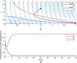
(a) A typical trajectory starting at tends to the unique stable equilibrium point corresponding to the low concentration level for v, (b) Time‐domain simulations of u and v for the unique equilibrium point
Fig. 2.
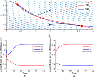
(a) Two different trajectories starting from different domains of attraction (at and ) and ending at two distinct stable equilibrium points and , (b), (c) Time‐domain simulations of u and v for three‐equilibrium point case
Fig. 3.
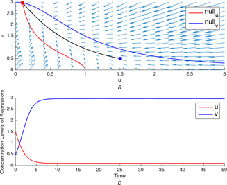
(a) A typical trajectory starting at tends to the unique stable equilibrium point where u is at a low‐concentration level, (b) Time‐domain simulations of u and v for the unique equilibrium point
In Figs. 1 a and 3 a, the production rates, and , are not balanced. In these cases, the nullclines intersect each other only ones and the intersection point is the stable equilibrium point locating at the high concentration level of the repressor protein, which is the one with the higher production rate. It can be seen in Figs. 1 b and 3 b, the repressor with higher rate goes to ON state at high concentration level while the other one goes to OFF state.
When the rates are balanced, the bistability occurs so that the steady‐state values of repressors depend on their initial levels as shown in Fig. 2 a. Herein, the separatrix divides the phase plane into two domains of attraction corresponding to two different stable equilibrium points. The concentration level reaches one of the stable equilibrium points depending on which domain of attraction the initial state is in.
In the monostable cases, the steady‐state values of the concentration levels of repressors are fixed due to the uniqueness of the equilibrium point. However, in the bistable case possessing the toggle mechanism, the steady‐state values of the concentration levels are not unique and depend on their initial values. For the model in (1) and (2), the (bistable) toggle switch mechanism requires the existence of three equilibriums, two of them stable and one unstable.
For possible realisation purposes in synthetic biology, it would be of interest to know the ranges of model parameters ensuring the toggle mechanism. Although the change of bistable/monostable behaviour of the model in (1) and (2) depending on the model parameters is analysed by finding time domain solutions of the related differential equations for some parameter values [7]. However, there is no study in the literature providing whole parameter ranges ensuring the bistability/monostability. Such a bifurcation analysis is conducted in this study based on studying the quantitative and qualitative properties of the equilibrium points for all the possible parameter values. In this context, first the root‐locus method is applied to find the parameter ranges resulting three equilibriums. Second, the stabilities of these equilibriums are checked in two different ways. The first method in the stability analysis is to check the eigenvalues of the Jacobian matrix, and the other one is the dynamic route (also called vector field) method [17, 22].
2.1 Quantitative equilibrium point analysis using the root‐locus method
The study of the number of equilibrium points in terms of the model parameters can be realised by considering the equilibrium equations. For the ODE model in (1) and (2) which are with rational right‐hand sides, one can obtain the equilibrium equation as a polynomial function of a state variable by imposing the steady‐state assumption () and then eliminating one of the state variables
| (5) |
So, as in [12], one can apply the well‐known root‐locus method of control theory, which is actually used for determining the change in the locations of closed‐loop poles of a linear time‐invariant feedback control system with respect to a certain parameter in complex s ‐plane. The root‐locus is applied to the characteristic equation of a control system schematised in Fig. 4 where K parameter is the proportional controller gain, the rational functions and of s complex variable are feed forward and feedback transfer functions in the Laplace domain, respectively. The usage of the root‐locus method in this work is completely different from the control applications. It is used here for studying the existence of the equilibrium points with respect to some parameters in contrast to the change of the positions of the closed‐loop poles.
Fig. 4.

Closed‐loop feedback system
To apply the root‐locus, we need to transform the polynomial equilibrium equation in (5) into a characteristic equation form. The characteristic forms for the model parameters and are given in (6) and (7), respectively
| (6) |
| (7) |
It is known that the equilibrium points of a non‐linear system are the real roots of the polynomial equilibrium equation. So, the equilibrium points of the models (1) and (2) can be obtained as the real roots of the characteristic forms in (6) and (7) with the identification of the real‐axis segments of root‐locus graph [7].
To determine the bistability parameter ranges of production rates and , let us first consider the case of the cooperativity degrees as . Then, the equilibrium equation in (6) and (7) can be rewritten as follows:
| (8) |
| (9) |
The equilibrium points of the toggle switch model in (1) and (2) for and parameters lie on the real‐axis segments of root‐locus graphs drawn for the positive and negative feedback systems in (8) and (9), respectively. The fifth‐order polynomial equilibrium equation has always two complex roots as conjugate pairs. The other three roots become real or complex depending upon the values of and parameters. One of these three roots is necessarily real for all choices of and . As can be seen from the stability analyses in Section 2.2, when the equilibrium equation for the models (1) and (2) has a single equilibrium point, this equilibrium point has to be asymptotically stable and also the bistability necessitating three equilibrium points does not occur. To determine the bistability parameter range, one should obtain the parameter values for which the equilibrium equation has two more real roots in addition to the ever existing one.
The MATLAB graphs for and parameters are shown in Figs. 5 and 6, respectively. The parameter range in which the equilibrium equation has three real roots is the intersection of three distinct parameter intervals each of which is the set of parameter values yielding the real segment of the branch associated with a root. The number and position of the equilibrium points are, indeed, functions of only two independent parameters ( and ) since and are held fixed. The finding of the parameter values providing three equilibrium points is the problem of determining a region in the two‐dimensional parameter space consisting of pairs at which the equilibrium equation has three real roots. Such a two‐dimensional parameter region can be obtained in the following way: firstly, for a chosen parameter (e.g. ), the parameter intervals yielding three real roots are determined by exploiting the root‐locus graphs when the other parameter () is held fixed at different specific values. The intervals of parameter obtained for different choices of are then combined.
Fig. 5.
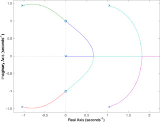
Fig. 6.
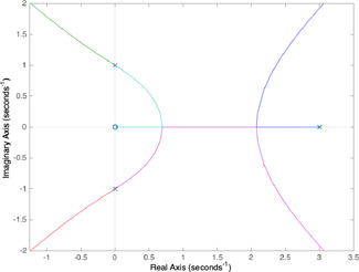
Following the above‐mentioned procedure, for the choice of , the parameter intervals of where the roots become real are, respectively, obtained as [0, 3.54], [2.71, 3.54], and [2.71, inf) for the first, second, and third branches of root‐loci depicted in Fig. 5. In the first branch, the pole locates at origin for and it takes real values until and then it starts to get complex values. In the second branch, the pole initialising at a pure complex value becomes a real root when is between 2.71 and 3.54. In the third branch, the pole starting as a complex root becomes real when . As can be seen from Fig. 5, the equilibrium equation has three roots for which is the intersection of three distinct intervals explained above. By applying the same procedure for parameter, the intersection of three intervals [0, 12.5], [7.29, 12.5], and , which are obtained similarly to the ones for is found as [7.29, 12.5] when is held fixed at 3 (see Fig. 6). Despite the fact that the characteristic equation form for expresses positive feedback, the characteristic equation for contains as a control parameter and also expresses negative feedback. When we take the square roots of the boundary values of the parameter range obtained for , it can be seen that they are the same as the ones found for parameter. This result, which is a direct consequence of the facts that (8) and (9) are actually the different forms of the same equilibrium equation and and are chosen as identical (), is consistent with the result in [7] related to the balanced rates reported to be needed for the existence of the bistability.
By repeating the above way of determination of the parameter range of for , the two‐dimensional parameter region providing the existence of three equilibrium points was obtained. The parameter values that guarantee the bistability were determined by detecting the parameter values yielding one unstable (repeller) and two stable (attractors) equilibrium points with the stability analysis given in Section 2.2. As can be seen from the vector field approach described at the end of Section 2.2, the region of parameter values providing the existence of three equilibrium points completely coincides with the bistability region.
2.2 Qualitative equilibrium point analysis based on the eigenvalues of the Jacobian matrix
The bistability analysis of the genetic toggle switch, which is started in Section 2.1 with the quantitative analysis of determining the number of equilibrium points, is completed in Section 2.2 by a qualitative analysis based on the Lyapunov stability of these equilibrium points. The necessary and sufficient condition for the Lyapunov stability of an equilibrium point for a linear system is that the eigenvalues of the equilibrium point lie in the closed left‐half plane and pure imaginary eigenvalues (if any) have multiplicity one, i.e. simple. The existence of simple pure imaginary eigenvalues means that the equilibrium point is marginally stable, and the case of eigenvalues whose real parts are all strictly less than zero indicates an asymptotically stable equilibrium point. To check the stability of the three equilibrium points of the non‐linear system in (1) and (2), which is obtained from root‐locus graphs, we calculated the eigenvalues of the Jacobian matrix evaluated at each of these equilibrium points.
The Jacobian matrix of the toggle switch model in (1) and (2) is derived in the first step of the stability analysis
| (10) |
Then, the eigenvalues ('s) of the Jacobian matrix evaluated at the equilibrium point with can be calculated as follows:
| (11) |
where and z is defined as
The eigenvalues of the toggle switch model are then determined by finding the roots of the characteristic equation given in (11)
| (12) |
The Routh–Hurwitz stability test can be applied to decide if there exists an eigenvalue in the open right‐half plane and/or a pure imaginary eigenvalue with the multiplicity more than one for an equilibrium point . The Routh array is constructed as in Table 1. The sign change in the first column of the Routh table indicates the existence of an eigenvalue in the open right‐half plane, implying the instability of the equilibrium point. Equation (12) and the sign change condition gave the same result, as being of z strictly <1, for the asymptotic stability of the equilibrium points. One can reach the same result from (12).
Table 1.
Routh array for the characteristic equation of the toggle switch model
|
|
1 |
|
||
|
|
2 | — | ||
|
|
|
— |
The bistability region in two‐dimensional space is obtained by applying first the root‐locus method to obtain the parameter region providing three equilibrium points and then, by applying the Routh–Hurwitz test to check the stabilities of these equilibrium points. The bistability region obtained by the root‐locus based method is computed in two‐dimensional parameter space for as shown in Fig. 7. The study in [7] reported that the bistability region of the model in (1) and (2) has a cone‐like shape in logarithmic scale such that its boundaries are both exponential for small and and they tend to be linear for large and . Herein, the slopes of upper and lower boundary lines were given as and , respectively.
Fig. 7.
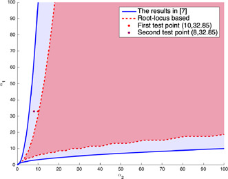
For , the comparison of two bistability regions obtained for genetic toggle model: one of them is the bistability region obtained by the root‐locus based analysis and the other one is found in [7 ]. The test points are chosen to check the bistability regions
To compare the bistability regions in two‐dimensional parameter space, the boundaries for the method in [7] are also drawn in Fig. 7. It can be seen that the bistability region obtained by the root‐locus based analysis is narrower than the region given in [7] for all and values. In other words, the analysis by Gardner et al. [7] reported the bistability for any parameter pair inside the bistability region determined by our root‐locus‐based analysis, but the reverse is not true, i.e. our analysis method does not find the models (1) and (2) as bistable for some parameter pairs that are claimed in [7] to yield the bistability.
To clarify the conflict between the results obtained by the above‐mentioned two different analyses, the following four methods other than the conflicting ones are applied below for some test points: (i) the first method is to calculate how many equilibriums points the equilibrium equation in (5) has for test points. (ii) The second method is to draw the nullclines to identify their intersections defining the equilibrium points and to conduct simulations for different initial conditions to check the qualitative properties of these equilibrium points again for the same test points. (iii) The third one is a graphical method, i.e. the application of the vector field approach again to determine how many equilibriums points the model in (1) and (2) has for the test points, and how many of those equilibrium points are stable and/or unstable. (iv) The last method is actually the combination of the first three ones. It aims to compare the boundaries of the bistability regions, which are obtained for different parameters. Thus, it will be checked if the slopes of the boundaries of the bistability region are simple functions of and parameters as claimed in [7]. In view of the results obtained by the four validation methods, the bistability occurs for all of the test points inside the bistability region computed by the root‐locus‐based analysis while it does not occur for the test points placed at the conflicting section between the bistability regions.
The test points are chosen arbitrarily as (32.85, 10) and (32.85, 8) such that the first one lies on the boundary of the bistability region found by the root‐locus‐based analysis and the second, which is very close to the first one, inside the conflicting section.
To calculate the roots of the equilibrium equation for , (5) is rewritten as follows:
(13)
For two test points, (32.85, 10) and (32.85, 8), the roots of the equilibrium equation in (13) are computed by using roots function in MATLAB. The fifth‐order polynomial equation in (13) has four complex conjugates roots and a single real root when the test point is chosen from the conflicting section between two bistability regions. Opposite to the results in [7], the uniqueness of the real root, which is at , means that the bistability does not occur since there is just a single equilibrium point. For the test point (32.85, 10) on the boundary of the bistability region found by the root‐locus‐based analysis, there are one complex pair and three real roots locating at , so the first condition for the bistability is seen to be met. With the help of the stability analysis, for the test point (32.85, 10), one of the three equilibrium points is found as unstable and the other two ones are as asymptotically stable. The similar computations, which are done for the other test points chosen from the conflicting section and from the bistability region found by the root‐locus‐based method, confirm the validity of the root‐locus‐based bistability analysis.
For the test point (32.85, 8) from the conflicting section, the nullclines drawn in Fig. 8 a indicate that the model in (1) and (2) again behaves as monostable with the unique stable equilibrium point locating at the intersection of two nullclines. The monostable behaviour is also seen from the time domain simulations in Figs. 8 b and c conducted for different initial conditions.
Fig. 8.
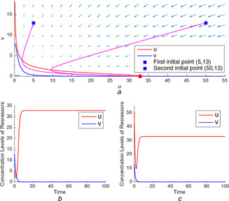
Genetic toggle model's nullclines and time‐domain simulations for the test point (32.85, 8)
(a) Trajectories starting from two different initial points end at the same unique equilibrium point, (b) Time‐domain simulation for the initial point , (c) Time‐domain simulation for the initial point
As can be seen from Fig. 9 a, the nullclines intersect each other three times that means there exist three equilibrium points for the test point (32.85, 10). The separatrix passing through the unstable equilibrium point divides the two‐dimensional parameter space into two distinct domain of attractions. For two initial points starting from two different domains, the simulation results expose the bistable behaviour of the toggle model through the different concentration levels of model variables, u and v, at the steady state as seen in Figs. 9 b and c, respectively.
Fig. 9.
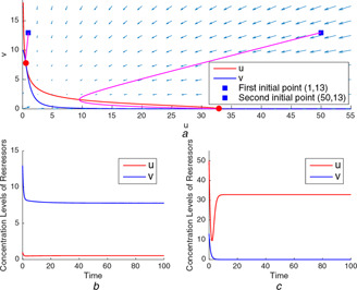
Genetic toggle model's nullclines and time‐domain simulations for the test point (32.85, 10)
(a) Trajectories starting at two initial points from different domains end at two different equilibrium points, (b) Time‐domain simulation for the initial point , (c) Time‐domain simulation for the initial point
The third validation method is the vector field approach, which is used to determine the number of equilibrium points and their qualitative properties by plotting the derivative of a state variable versus itself. The variable v is eliminated first by equating (2) with zero and then by substituting the expression of v obtained in the first step into (1). To compare the results for the same test points, the vector field graphs of are drawn for these parameter values. For the test point (32.85, 8) chosen from the conflicting section, the vector field graph in Fig. 10 shows that the model in (1) and (2) again has a unique equilibrium point which is asymptotically stable. For the test point (32.85, 10), together with the arrows showing the directions of the trajectories, the three equilibrium points, two of which are seen by zooming the initial portion of the graph in Fig. 11, indicate the bistability of the model.
The fourth method is used to test whether or not the boundaries of the bistability region are simple functions of and parameters. It is claimed in [7] that the slopes of the boundaries are as and both in logarithmic scales. To examine if there is any difference between the boundaries of the bistability regions obtained by keeping one of the beta and gamma values constant and changing the other one, first we calculate the whole bistability region for again. Second, we fix to 2 and take as 1 to determine the new bistability region. Owing to the same value, there must be no difference between the upper bound of these two bistability regions if the statement in [7] is true. A similar comparison is made for the lower bounds by keeping the value as 2 and changing value to 1. According to [7], there should be no difference between the lower bounds of the bistability regions. However, this is not the case: as seen from Fig. 12, the upper and lower bounds of the bistability regions change as functions of two parameters and not the single parameter as claimed by Gardener et al. [7].
Fig. 10.
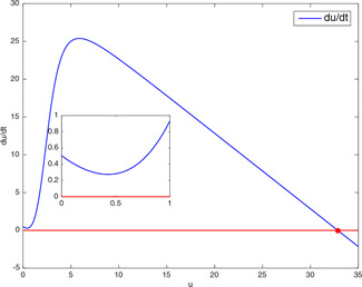
Vector field graph ( versus u) of genetic toggle model having only one stable equilibrium point for the test point (32.85, 8)
Fig. 11.
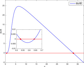
Vector field graph (u versus ) of genetic toggle model having two stable and one unstable equilibrium points for the test point (32.85, 10)
Fig. 12.
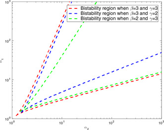
Dependency of the boundaries of the bistability regions found by the root‐locus‐based analysis for genetic toggle model on the and parameters: the bistability region is computed for , first. The bistable region lies inside each pair of curves. Then, two different bistability regions are also calculated: the first one is bistability region for and and the second one for and
As a conclusion, the root‐locus‐based analysis determines the exact bistability region in contrast to the one in [7]. The difference might be a consequence of over‐simplification of the boundaries of the bistability region or miscomputation in solving ODEs.
The proposed root‐locus‐based analysis is applied also for and cooperativity degrees other than 2. The corresponding bistability regions in the two‐dimensional parameter space are depicted in Fig. 13. It is seen that the smaller the cooperativity degrees get, the narrower the bistability region gets. Thus, the higher cooperativity degrees guarantee the larger bistability region in parameter space as similar in the study of Gardner et al. [7].
Fig. 13.
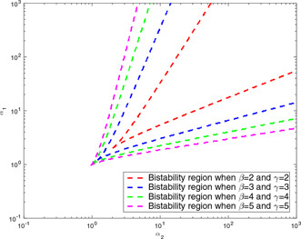
Bistability region found by the root‐locus‐based analysis for genetic toggle model with different and values: increasing the cooperativity degrees of repression ( and ) enlarges the size of the bistable regions. Bifurcation lines are depicted for four different values of and
3 Bifurcation analysis of the p53 gene regulatory network model of polynomial type
p53, also known as TP53 or tumour suppressor, is a gene that controls the cell cycle by regulating complicated pathways. It was first introduced in 1979 by Soussi [23], but its role as a tumour suppressor was revealed later in 1989. p53 gene regulatory network including p53 gene plays a pivotal role since it regulates the cell division to prevent the cell proliferation by checking the mutation in DNA during the different phases of the division process [24]. In the routine controls along cell cycle, when the mutation caused by ionising radiation (IR) [25, 26] is detected by the p53 gene regulatory network, it first attempted to repair the double strand breaks (DSBs) in DNA. In order to activate the DNA damage repair mechanism [27] through cell cycle arrest, the concentration of p53 protein, which is at low‐level state in normal conditions [28], starts to oscillate [29]. If the damage is small and could be fixed into a heritable mutation, cell cycle continues after the second control while the concentration level of p53 decreases to low level again. When the DNA damage is too high to be repaired, the cell goes apoptosis. While stopping the cell cycle permanently, the concentration level of p53 is boosted to a high‐level state to activate the mechanism causing the cellular senescence [30–32]. Thus, the p53 gene regulatory network acts in three different ways for the regulation of the cell response to DNA damage [25, 31]. These three distinct behaviours, namely a low‐level state, oscillation, and a high‐level state, correspond to normal unstressed condition, cell cycle arrest, and apoptosis, respectively.
The p53 gene regulatory network has been the most studied gene network since its vital role to suppress cancer was discovered. There are many different mathematical models to explain the above‐mentioned three distinct modes of the p53 gene network [10, 26, 33]. Owing to the number of the components and the complexity of the relations among them, the mathematical models are a bit complicated since they are defined by a high number of state variables and highly non‐linear functions. Failing to capture the essential mechanisms and critical interactions is a disadvantage for these high‐dimensional models. The non‐linearities in the models make the analysis complicated and sometimes impossible. Owing to its low dimensionality and simplicity in the non‐linear interactions, the two‐dimensional polynomial type oscillator model of Demirkran et al. [10] is chosen in this study to analyse the exact ranges of the model parameters ensuring the three modes of the p53 network.
The two‐dimensional polynomial type canonical relaxation oscillator model given in (14)–(16) is introduced in [10] by following a minimalist approach to describe the qualitative behaviours of the p53 gene network. The p53 model in (14)–(16) includes two state variables, x and y, which represent the concentration levels of and proteins, respectively. The reason for choosing these two variables is that , , and their interaction plays essential roles in the p53 network dynamics. As explained in [10], this two‐dimensional model of the p53 network that takes and as state variables comprise two constitutive mechanisms, namely and negative feedback loop and the positive feedback of into itself causing the bistable behaviour. Since the concentration level of p53 protein is known to be directly proportional to the concentration level of , p53 could be assumed as a hidden variable by taking as a state variable
| (14) |
| (15) |
| (16) |
In the models (14)–(16), the state variables x and y, respectively, represent the and concentrations. The model parameters a, b, c, d, n, z, , and are positive constants and m is assumed to be non‐negative. and are time constants and can be neglected in the steady‐state analysis. The parameter r indicates the severity of the DNA damage and could take values between 0 and 1. Thus, the DNA damage can be applied as an external input signal to the model by setting it to a constant level. The parameter m represents the excitation of by and then, the existence of – negative feedback loop. When m is equal to zero, concentration saturates at the high‐level state due to the disappearance of the negative feedback. The inequality in (16) is required for the existence of a trapping region to exhibit the oscillatory behaviour when the DSBs reach a threshold value.
The equation in (14), which describes the change of the concentration of , includes a cubic term to provide the bistable behaviour resulted from the auto‐activation property of . It is known for ODE models that, for the existence of bistability, it is required to have two stable and one unstable, totally three equilibriums [12, 13]. The term appears when is needed for bistable behaviour of . This cubic term together with the term ‐ xab stands for the self‐degradation of . The cy ‐ d and terms, both of which arise when , generate the oscillatory behaviour of . The negative term ‐ cxy corresponds to the strong inhibitory relation between and . On the other hand, two positive terms and rdx explain the auto‐activation property of , which causes rapid responses to DSBs.
The second equation in (15) describes the change of the concentration of protein. The first term z indicates the constant production rate. The second term mx represents the activation of by when m is not equal to zero. It means the can regulate itself via self‐inhibition through in an indirect way. It explains that there is no activation between and , when and the inhibitory effect of on gets smaller to reach a high‐level of concentration due to high level of IR exposure. The last term ‐ ny in (15) stands for the self‐degradation.
Bifurcation analysis in terms of r and m parameters : The severity of the DNA damage and the activation weight of on , respectively, r and m, are chosen in [10] as the adjustable parameters to present different scenarios corresponding to three distinct behaviours of the p53 network. It is assumed in [10], the parameter values are . The parameter m is set 0 and 1.25 to obtain low‐level equilibrium state and high‐level equilibrium or oscillation according to the severity of DNA damage, respectively. The severity parameter r is defined as , which possesses a saturation property. Here, represents the number of double strand break complexes formed by DNA repair molecules with DSBs during IR exposure. In [10], the parameter r is taken as either 0 or 1. The combinations of parameters m and r are given as for the low‐level state, oscillation and high‐level state, respectively, in [10]. As stated in [10], these specific parameter values are chosen only to show that the model is capable of explaining three different modes. These values are not enough to see the whole picture about the ranges of the parameters ensuring three distinct behaviours of the p53 network. In the sequel of this paper, by applying a thorough analysis similar in toggle switch case, the exact parameter ranges for m and r providing three qualitative behaviours of the p53 gene regulatory model in (14) and (15) are explored. Choosing m and r as bifurcation parameters in this study relies on the fact that these two parameters are the determinant factors of the p53 network; r is the driving input and m adjusts the strength of the – negative feedback loop controlling the behaviour of the network. By the way, the study can be extended in a straightforward way to include the other parameters in the bifurcation analysis.
For three different combinations of parameters m and r given in [10], the dynamical behaviours of the model in (14) and (15), which correspond to three distinct modes, are examined by drawing the nullclines as depicted in Figs. 14, 15–16. For the considered values of the parameters, the concentration levels of and proteins are computed as in Figs. 14b, 15b, and 16 b by solving equations in (14) and (15). The dynamical behaviours of the model change depending on the qualitative and quantitative properties of the equilibrium points, namely their locations and stabilities, which are indeed the intersections of the nullclines. As in [10], let us analyse the properties of the equilibrium points to give an insight into the behaviour of the p53 network. To do that first, the nullclines of two state variables x and y are derived by assuming and as given in (17)–(19). Then, the quantitative and qualitative properties of the intersection points of the nullclines are examined. In this case, the model has three nullclines, two of which belong to the state variable x, and the last one belongs to the state variable y
| (17) |
| (18) |
| (19) |
The first nullcline, , is irrespective of all the parameters. The degree of the second nullcline, , and the number of its intersection points with the third nullcline, , change with respect to the parameter r. When , (18) defines a horizontal line as . The third nullcline, , defines a line whose slope depends on the parameter m which represents the strength of the – negative feedback loop. When , which means almost no inhibition on by , the slope of is equal to zero and it turns into a horizontal line, which is .
Fig. 14.
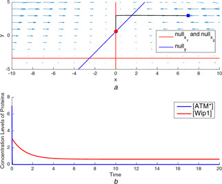
Nullclines and time‐domain simulations for p53 gene regulatory network model with different parameter sets
(a) A typical trajectory tending to the stable equilibrium point at a low‐concentration level of , (b) Time‐domain simulations of and for the equilibrium point at a low concentration level of
Fig. 15.
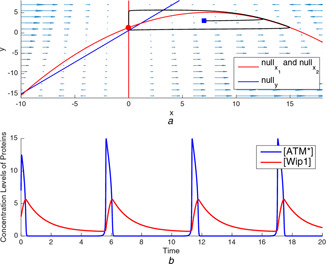
Nullclines and time‐domain simulations for p53 gene regulatory network model with different parameter sets
(a) Oscillatory dynamics, (b) Time‐domain simulations of and for oscillatory case
Fig. 16.
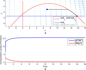
Nullclines and time‐domain simulations for p53 gene regulatory network model with different parameter sets
(a) A typical trajectory tending to the stable equilibrium point at a low‐concentration level of , (b) Time‐domain simulations of and for the equilibrium point at a low concentration level of
The nullclines are shown in Fig. 14 a for the parameter values providing the low‐level equilibrium state. It can be seen that the defines a horizontal line, , and the intersects with and at two different points corresponding to two distinct equilibrium points. Since the state variables represent the concentration levels of and proteins, the equilibrium point in the third quadrant is not valid for the model in (14)–(16) and this equilibrium point is also obtained as a saddle point by the stability analysis. As given in [10], the stability analysis based on the eigenvalues of the Jacobian matrix evaluated at the equilibrium point explains that the second equilibrium point at is asymptotically stable in the sense of Lyapunov. It is shown in Figs. 14 a and b that a trajectory started from the initial point ends at the asymptotically stable equilibrium point at (0, 0.625). The concentration level of protein goes to the low‐level state which means that the concentration level of p53 protein is also at low‐level state when there is no DNA damage in the cell, which means .
The nullclines in Fig. 15 a display the equilibrium points result the oscillations in the concentration levels of the proteins. The parameter conditions are assumed to be as given in [10]. For this parameter set, the model in (14)–(16) has three equilibrium points one of which is asymptotically stable in the sense of Lyapunov. However, this stable equilibrium point is always in the third quadrant, so not valid again. The stability analysis shows that one of the other two equilibrium points, which are at , is always a saddle point. The stability analysis shows that there is always a unique equilibrium point in the first quadrant under the constraint in (16). The position and stability of the third equilibrium point depend on the values of parameters and and the degradation term n of y. The oscillations occur when it is unstable in the sense of Lyapunov. In other words, stability destroys the oscillations. The required condition for the stability of the equilibrium point is obtained as the position of the equilibrium point is above the peak value of curve. In Fig. 15 a, it is observed that the trajectory started from the same initial point with the simulation in Fig. 14 a oscillates due to the existence of the unstable equilibrium point. The concentration levels of and protein oscillate to arrest cell cycle for the activation of the DNA damage repair mechanism when the maximum severity of the DNA damage and strong negative feedback conditions occur together.
The illustrations in Figs. 16 a and b depict the high‐level equilibrium state case for high DNA damage in the cell without negative feedback loop between and . The parameter combination is taken as , which is given in [10] for yielding high DNA damage. Again, one of the equilibrium points in the third quadrant is not a valid solution for the model in (14)–(16). The stability analysis explains the existence of an asymptotically stable equilibrium point for the high levels of concentration and the saddle point for the low level of concentration both of which cause the high‐level equilibrium state as the severity of the DNA damage gets higher. As shown in Fig. 16 b, the parameter setting with the same initial point now results in the high‐level concentration, which yields the cell apoptosis due to the high DNA damage.
The simulation results in Figs. 14, 15–16 show that the proposed two‐dimensional polynomial type canonical relaxation oscillator model in (14)–(16) is capable of explaining the three distinct behaviours of the p53 gene regulatory network. As stated before, only some parameter values which provide these behaviours are given in [10]. Similar to the toggle switch model analysis done in Section 2, the two‐stage bifurcation analysis will be applied to the p53 gene network model in (14)–(16) to determine the whole parameter ranges ensuring the low‐level, oscillatory, and high‐level states in Section 3. The number of the equilibrium points of the models (14)–(16) will be obtained in the root‐locus‐based quantitative analysis stage of the bifurcation analysis and then, the stabilities of these equilibrium points in terms of the eigenvalues of the Jacobian matrix will be examined in the qualitative analysis stage. Based on such an analysis, the two‐dimensional m and r parameter space will be divided into three distinct regions corresponding to these parameter ranges that provide the three different behaviours.
3.1 Quantitative equilibrium point analysis using the root‐locus method
The bifurcation analysis starts with the root‐locus‐based quantitative analysis stage to identify the number of equilibrium points for each specific parameter set. Under the steady‐state assumption , the third‐order polynomial equation in (20) is obtained by eliminating the second state variable y as the equilibrium equation for the p53 model in (14)–(16)
| (20) |
Owing to their principal roles on the dynamics, the p53 gene regulatory network model in (14)–(16) is analysed in terms of the model parameters r and m, which correspond to the severity of DNA damage and the strength of the auto inhibition of via , respectively. For these model parameters r and m, the characteristic equations in (21)–(22) can be derived from (20) to apply the root‐locus based analysis
| (21) |
| (22) |
The parameter r can take values between 0 and 1. However, only the limit cases representing the minimum and maximum DNA damages are taken into account in [10]. Similarly, the analyses in [10] consider only two specific values, namely 0 and 1.25, for the parameter m. These lack the information about the whole ranges of the parameters r and m causing a dynamical mode of the model in (14)–(16). In this study, to obtain the parameter ranges ensuring the different model behaviours in r ‐ m parameter space, the root‐locus method is applied to (21) by choosing m as a control parameter and fixing r at a specific value between 0 and 1 in each case. It should be noted that the same parameter regions in r ‐ m space can be obtained also by using the characteristic equation (22) written for the control parameter r.
It can be seen from Fig. 17 that, for the parameter value set , the branches of the root‐loci for m start at the open loop poles of the characteristic equation (21) and tend to the open loop zeros, one of which is at the infinity. One of the branches starts at the origin and stays there for all m values. The second branch starts at the real pole 1.06 and goes to the finite zero at the origin while the third one starting at the real pole 13.9 tends to the zero at the infinity. The other two real poles turn into a complex conjugate pair when m is between 0.273 and 0.847 which means that the model in (14)–(16) has a single equilibrium point for these m values and three equilibrium points for the other m values.
Fig. 17.
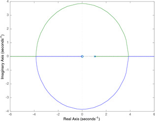
Typical root‐locus graph obtained for the parameter m when r is held at 0.7
The p53 gene regulatory model in (14)–(16) may have one, two or three equilibrium points based on the values of the parameters r and m. Obtaining the root‐locus plots for m holding r at a specific value, the parameter regions for different numbers of the equilibrium points of the model in (14)–(16) are determined as given in Fig. 18. Seven disjoint simply connected regions, each corresponding to a different number of equilibrium points and/or qualitative properties, are identified in the r ‐ m parameter space. The quantitative analysis stage of the bifurcation analysis together with the qualitative one to be presented in Section 3.2 which constitutes the second main contribution of this study extends the work in [10].
Fig. 18.
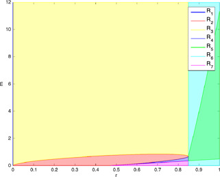
r ‐ m parameter regions for different modes where the union of , , , and regions corresponds to low‐level state, region corresponds to oscillatory state, region corresponds to high‐level state and region corresponds to bistable mode
The model in (14)–(16) has a single equilibrium point for the parameters in region and three equilibrium points in the union of , , , , and regions of Fig. 18. As also stated in [10], the model has two equilibrium points on the red vertical line in region. To identify the dynamical behaviour of the model, the stability analyses of these equilibrium points are made by calculating the eigenvalues of the Jacobian matrix evaluated at the related equilibrium points. The parameter regions shown in Fig. 18 corresponding to the different modes of the model in (14)–(16) are determined based on the number of the equilibrium points calculated in this section combined with the stability analyses of these equilibrium points conducted in Section.3.2.
3.2 Qualitative equilibrium point analysis based on the eigenvalues of the Jacobian matrix
In the qualitative analysis part, first, the Jacobian matrix of the model in (14)–(16) is derived to get the information about the stabilities of the equilibrium points obtained in the previous stage
| (23) |
where z is defined as .
The time constants and are both assumed to be equal to 1 as in [10]. Then, the eigenvalues ('s) of the Jacobian matrix evaluated at the i th equilibrium point can be calculated by solving the second‐order polynomial equation in (24)
| (24) |
where .
Depending on the quantitative and qualitative properties of the equilibrium points, the required conditions for a specific dynamical behaviour are derived. Then, according to these conditions, the r ‐ m parameter space is subdivided into the different regions as shown in Fig. 18. Each region in Fig. 18 corresponds to a different mode of the p53 gene regulatory model. The analyses in [10] are made only to show that the model in (14)–(16) is capable of explaining the three different modes of the p53 gene networks for specific parameter value sets. In contrast, this study presents the whole parameter regions, which are shown in Fig. 18, causing the low‐level state, the high‐level state and the oscillatory modes of the p53 gene networks. In addition to these regions corresponding to the three modes already presented in [10], a new parameter region related to a bistable behaviour is also identified. The required conditions related to the quantitative and qualitative properties of the equilibrium points for each mode will be explained in the sequel.
3.2.1 Low‐Level state (normal unstressed cell)
When there is no DNA damage or the severity of the DNA damage is low, the cell stays in normal unstressed mode and the concentration level of , also p53 protein, is in low level. In [10], only the case of under the condition of no DNA damage, namely , is studied for the low‐level state. For and , the model in (14)–(16) has two equilibrium points, one of which lies on the second or third quadrant, so invalid, and the other one, which is at , is asymptotically stable [10]. By the presented root‐locus based bifurcation analysis, four different sub regions of the r ‐ m parameter space any of which defines a low‐level state but with different numbers of equilibrium points or different stability properties are identified.
The quantitative and qualitative properties for these sub regions, which are summarised in Table 2, are described in the sequel.
Table 2.
Conditions for low‐level state
| Possible cases | Quantitative properties | Qualitative properties | |
|---|---|---|---|
| two equilibriums case |
|
asymptotically stable | |
| with | asymptotically stable | ||
| single equilibrium case |
|
asymptotically stable | |
| three equilibriums case I |
|
asymptotically stable | |
| with | saddle | ||
| with | asymptotically stable | ||
| three equilibriums case II |
|
asymptotically stable | |
| with | saddle | ||
| with | unstable |
Two equilibriums case : The root‐locus analysis shows that two equilibrium points exist with the properties given in the first row of Table 2 for regardless of the m value. It should be noted that the point given in [10] lies on the obtained one‐dimensional region () defined by the vertical line segment with . For all parameters in this region, one of the equilibrium points, which lies on the second or third quadrant, is again invalid. The other one, which is at , is asymptotically stable, all the trajectories starting in the first quadrant ends at this equilibrium point , eventually leading low (actually zero) level of x ( concentration).
Single equilibrium case : For the parameters from region, the model is found by the root‐locus analysis to have only one equilibrium point at . The qualitative analysis shows that this equilibrium point corresponding to the low‐level state again is asymptotically stable, attracting all trajectories starting in the first quadrant.
Three equilibriums case I : There exist three equilibrium points of the model in (14)–(16) for the parameters from region. One of these equilibrium points is at and the other two of them are invalid since taking place at the second or third quadrants. Only the possible equilibrium point is at and the eigenvalue‐based stability analysis shows that it is an asymptotically stable one attracting all trajectories starting in the first quadrant.
Three equilibriums case II : For the parameters in region, the model in (14)–(16) has three equilibrium points all in the first quadrant. One of them is again at . The second one is always a saddle point and the third one is unstable. All trajectories end at the stable equilibrium point when they start in the first quadrant excluding the other two equilibrium points (Table 3).
Table 3.
Conditions for oscillatory state
| Possible case | Quantitative properties | Qualitative properties | |
|---|---|---|---|
| three equilibrium case |
|
saddle | |
| with | asymptotically stable | ||
| with | unstable |
3.2.2 Oscillation (cell cycle arrest)
In [10], the oscillatory state is obtained under the coexistence of the maximum severity of the DNA damage and the strong auto‐inhibition of via provided that . For these parameters, there exist three equilibriums; one of them is again at , which is a saddle point. The second one is an asymptotically stable equilibrium point, lying in the second or third quadrant, so invalid. The third equilibrium point is in the first quadrant and unstable. The analysis in [10] shows that the model in (14)–(16) has a relaxation type (asymptotically stable) oscillation around the unstable equilibrium point such that it is destroyed only for the initial conditions on the vertical axis of the phase space defining the stable manifold of the saddle point .
By the proposed root‐locus‐based bifurcation analysis, the exact parameter region corresponding to the above‐mentioned relaxation oscillation is determined. For the parameters in region, the model in (14)–(16) has three equilibrium points whose quantitative and qualitative properties are the same as those for and .
3.2.3 High‐level state (apoptosis)
It is reported in [10] that , which means the maximum DNA damage, together with , which means no auto‐inhibition of via , result in the high‐level state. The high‐level of the concentration causes that the concentration of p53 protein is also at the high level and the cell goes to apoptosis mainly due to the high DNA damage. It is stated in [10] that the model for and has three equilibrium points. The first one which is at is a saddle point. The second one is in the third quadrant and asymptotically stable, so again invalid. The third equilibrium point is in the first quadrant and asymptotically stable. Thus, all the trajectories go to the asymptotically stable equilibrium point when they start in the first quadrant excluding the vertical axis defining the stable manifold of the saddle point .
By the root‐locus based bifurcation analysis, it is determined that the parameters from region result in the high‐level state. For these parameters, the model in (14)–(16) has three equilibrium points. The first one is at and saddle point. The second equilibrium point is the asymptotically stable one lying in the second or third quadrant, so invalid. The third one lying in the first quadrant is asymptotically stable and it attracts all the trajectories starting at a point in the first quadrant excluding the stable manifold of the saddle point (Table 4).
Table 4.
Conditions for high‐level state
| Possible case | Quantitative properties | Qualitative properties | |
|---|---|---|---|
| three equilibrium case |
|
saddle | |
| with | asymptotically stable | ||
| with | asymptotically stable |
3.2.4 Bistable state
The bistable state case for the p53 gene regulatory network model is not studied in [10]. The root‐locus‐based analysis shows that the model may go to a low‐level or high‐level state depending on the initial conditions for the parameter sets in region. There exist three equilibrium points, one of them is at and asymptotically stable. The other two equilibrium points are also in the first quadrant. The second one is asymptotically stable and the third one, which is the saddle point that separates the attraction domains of two asymptotically stable equilibrium points. The trajectory starting from an initial point in the first quadrant goes to one of the stable equilibrium points depending on which domain of attraction the initial point is located at. Thus, for the parameters in region, the model behaves in a bistable mode (Table 5).
Table 5.
Conditions for bistable state
| Possible case | Quantitative properties | Qualitative properties | |
|---|---|---|---|
| three equilibrium case |
|
asymptotically stable | |
| with | asymptotically stable | ||
| with | saddle |
A gallery of time domain solutions of the model in (14)–(16) for different parameters in the above‐mentioned regions can be seen in the Appendix.
Remark on the bifurcation of the dynamics in terms of the severity of the DNA damage : One of the main contributions in the study is the identification of the critical values for the severity of the DNA damage in p53 gene regulatory network. The results show that the severity of DNA damage is one of the main factors determining the behaviour of the cell. As seen in Fig. 18, the bifurcation analysis reveals that there are two crucial values of r to switch the model in (14)–(16) from one mode to another. Until the severity reaches 0.475, the cell stays in the low‐level state regardless of the m value. It can be observed that no matter what level of the auto‐inhibition of via the cell does not recognise the severity of the DNA damage as vital until it reaches this critical value, namely .
In the range , the cell may be in the low‐level state or behave in the bistable mode depending on the value of m. For the weak auto‐inhibition of via which corresponds to small m values, the cell will be in the bistable mode, so the steady state depends on the initial conditions. On the other hand, if there exists a strong auto‐inhibition of via , the cell will be in the low‐level mode, so can tolerate the DNA damage. Thus, the model behaves in the low‐level or bistable mode for the r values below 0.85. That means the cell may tolerate the DNA damage up to the threshold level of the severity depending on the strength of the auto‐inhibition of via .
When the severity of the DNA damage reaches the critical value (0.85), the concentration levels of and p53 proteins oscillate or stay in the high‐level state. Thus, the cell must arrest the cell cycle and activate the DNA damage repair mechanism. After cell cycle arrest, when the DNA damage cannot be repaired and the severity is still in the high level, namely , the cell goes to the apoptosis corresponding to the high‐level mode.
As a result, depending on the severity level of the DNA damage, the dynamical behaviour of the model in (14)–(16) can be predicted. The reverse implication is also true: depending on the dynamical mode of the cell, the interval of the severity can be determined.
Remark on the effect of the degradation of over the parameter range ensuring the oscillation : It is stated in [10] that larger values of the degradation rate of , namely n, and the time scale ratio, namely , can destroy the oscillation regardless of the other parameter values. The result obtained from the proposed bifurcation analysis also supports this claim stated in [10].
To examine the effects of the degradation term of on the dynamics of the p53 networks, the oscillatory parameter regions for different degradation rates are obtained. As shown in Fig. 19, the oscillatory parameter regions shift upward in r ‐ m parameter space for higher degradation terms, namely n. The range of the auto‐inhibition level of ATM via includes higher m values for the same severity level r when the degradation rate is increased. This shift can be explained as due to the higher degradation rate, the concentration level of decreases in the cell and also, the auto‐inhibition of via gets weaker. To have a similar inhibition effect by the small amount of the protein, the strength of the auto‐inhibition, namely m, must be increased. Thus, the oscillatory behaviour can be observed at the higher m values when the degradation rate is increased. As stated in [10], the reason of the difference in the dynamics of the cells under the same radiation level may be explained as the differences among the degradation rates of the cells [10].
Fig. 19.
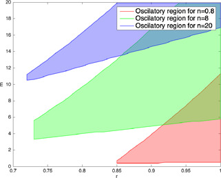
r ‐ m parameter regions for three different degradation rates
4 Conclusion
This study proposes the root‐locus‐based bifurcation analysis to determine the exact parameter regions ensuring the different dynamical behaviours of two different gene regulatory network models, namely the genetic toggle switch model and p53 gene regulatory network model.
The root‐locus‐based bifurcation analysis shows that the bistability region for the genetic toggle switch model gets larger when the cooperativity degrees, namely and , get bigger. Thus, the higher cooperativity degrees guarantee a larger bistability region in parameter space in accordance with the results in the literature. The most important result obtained for the genetic toggle switch is related to the boundaries of the bistable region. It is obtained that the upper and lower boundaries are both functions of and in contrast to the results in the literature.
As an extension of the current literature, for different dynamical modes of the considered polynomial type p53 gene regulatory network model, the whole parameter regions in r –m space are obtained in such a way that each sub region corresponds to a specific mode. So, it is obtained the threshold levels of the model parameters causing the changes in the dynamical behaviour of the model.
The parameter ranges obtained from the proposed analysis may help to explain the differences from one cell to another observed in the experiments. By exploiting the obtained results, it can be identified that how much of a difference between the parameters of a gene regulatory network model may cause the same dynamical mode or the completely different qualitative behaviours. So, the introduced bifurcation analysis would be highly beneficial whenever the biological phenomenon under investigation is described well by the analysed mathematical model.
The uncertainty in model parameters is the main challenge when obtaining an appropriate set of conditions for the emergence of desired dynamics in synthetic biology. The optimal parameter values play vital roles to guarantee the desired behaviour in biochemical processes. Furthermore, the robust experimental conditions and robust realisation of synthetic gene networks can be obtained by choosing the parameter values optimally, for instance by setting them to the centres of the found parameter regions.
The analysis can be applied to determine proper control inputs and their levels for deriving the gene regulatory networks in drug development studies. For instance, as shown for the p53 network in this study, the severity level of the DNA damage can be employed as a control input in a study related to cancer therapy and the critical threshold level of this control input can be determined. So, the required radiation level resulting in apoptosis for a cancer cell can be specified computationally by the proposed bifurcation analysis.
The aforementioned properties make the proposed analysis method as a favourable one for drug development, therapy design, and robust synthetic network design as well as the analysis of gene regulatory network dynamics.
5 References
- 1. Kitano H.: ‘Computational systems biology’, Nature, 2002, 420, pp. 206–210 [DOI] [PubMed] [Google Scholar]
- 2. Kitano H.: ‘Systems biology: a brief overview’, Science, 2002, 295, pp. 1662–1664 [DOI] [PubMed] [Google Scholar]
- 3. Angeli D. Ferrell J.E. Jr., and Sontag E.D.: ‘Detection of multistability, bifurcations, and hysteresis in a large class of biological positive‐feedback systems’, Proc. Natl. Acad. Sci., 2004, 101, pp. 1822–1827 [DOI] [PMC free article] [PubMed] [Google Scholar]
- 4. Murray J.D.: ‘Biological oscillators and switches’, in Antman S.S. (Ed.): ‘Mathematical biology I: an introduction’ (Springer, USA, 2007, 3rd edn.), pp. 218–256 [Google Scholar]
- 5. DiStefano J. III: ‘Dynamic systems biology modeling and simulation’ (Academic Press, UK, 2015, 1st edn.) [Google Scholar]
- 6. de Jong H.: ‘Modeling and simulation of genetic regulatory systems: a literature review’, J. Comput. Biol., 2002, 9, pp. 67–103 [DOI] [PubMed] [Google Scholar]
- 7. Gardner T. S. Cantor C. R., and Collins J. J.: ‘Construction of a genetic toggle switch in Escherichia coli ’, Nature, 2000, 403, pp. 339–342 [DOI] [PubMed] [Google Scholar]
- 8. Khalid M. Khan S., and Ahmad J. et al.: ‘Identification of self‐regulatory network motifs in reverse engineering gene regulatory networks using microarray gene expression data’, IET Syst. Biol., 2018, 13, pp. 55–68 [DOI] [PMC free article] [PubMed] [Google Scholar]
- 9. Demirkran G. Demir G.K., and Güzeliş C.: ‘Revealing determinants of two‐phase dynamics of p53 network under gamma irradiation based on a reduced 2‐D relaxation oscillator model’, IET Syst. Biol., 2017, 12, pp. 26–38 [DOI] [PMC free article] [PubMed] [Google Scholar]
- 10. Demirkran G. Demir G.K., and Güzeliş C.: ‘Two‐dimensional polynomial type canonical relaxation oscillator model for p53 dynamics’, IET Syst. Biol., 2018, 12, pp. 26–38 [DOI] [PMC free article] [PubMed] [Google Scholar]
- 11. Demirkran G. Demir G.K., and Güzeliş C.: ‘A canonical 3‐D p53 network model that determines cell fate by counting pulses’, Electrica, 2018, 18, pp. 284–291 [Google Scholar]
- 12. Avcu N. Alyürük H., and Demir G. K. et al.: ‘Determining the bistability parameter ranges of artificially induced lac operon using root‐locus method’, Comput. Biol. Med., 2015, 61, pp. 75–91 [DOI] [PubMed] [Google Scholar]
- 13. Avcu N. Demir G., and Pekergin F. et al.: ‘Discriminant‐based bistability analysis of a TMG‐induced lac operon model supported with boundedness and local stability results’, Turk. J. Electr. Eng. Comput. Sci., 2016, 24, pp. 719–732 [Google Scholar]
- 14. Avcu N. Pekergin N., and Pekergin F. et al.: ‘Aggregation for computing multi‐modal stationary distributions in 1‐D gene regulatory networks’, IEEE/ACM Trans. Comput. Biol. Bioinf., 2018, 15, pp. 813–827 [DOI] [PubMed] [Google Scholar]
- 15. Avcu N. Pekergin N., and Pekergin F.: ‘Coexistence of deterministic and stochastic bistability in a 1‐D birth‐death process with Hill type nonlinear birth rates’, in Sanayei A. et al. (Eds.): ‘ISCS 2014: interdisciplinary symposium on complex systems’ (Springer, Switzerland, 2015, 1st edn.), pp. 77–86 [Google Scholar]
- 16. Ozbudak E.M. Thattai M., and Lim H.N. et al.: ‘Multistability in the lactose utilization network of Escherichia coli ’, Nature, 2004, 427, pp. 737–740 [DOI] [PubMed] [Google Scholar]
- 17. Strogatz S.H.: ‘Nonlinear dynamics and chaos: with applications to physics, biology, chemistry and engineering’ (CRC Press, USA, 1994, 1st edn) [Google Scholar]
- 18. Meijer H.: ‘Matcont tutorial: ode gui version’, 2016.
- 19. Suarez R. Alvarez‐Ramirez J., and Aguirre B.: ‘First harmonic analysis of planar linear systems with single saturated feedback’, Int. J. Bifurcation Chaos, 1996, 6, pp. 2605–2610 [Google Scholar]
- 20. Aguirre B. Alvarez‐Ramirez J., and Fernandez G. et al.: ‘First harmonic analysis of linear control systems with high‐gain saturated feedback’, Int. J. Bifurcation Chaos, 1997, 7, pp. 2501–2510 [Google Scholar]
- 21. Aguirre B. Alvarez‐Ramirez J., and Suarez R.: ‘Symmetry breaking of periodic orbits in control systems: an harmonic balance approach’, Int. J. Bifurcation Chaos, 1998, 8, pp. 2439–2448 [Google Scholar]
- 22. Chua L.O. Desoer C.A., and Kuh E.S.: ‘Linear and nonlinear circuits’ (McGraw‐Hill, USA, 1987, 1st edn.) [Google Scholar]
- 23. Soussi T.: ‘The history of p53’, EMBO Rep., 2010, 11, pp. 822–826 [DOI] [PMC free article] [PubMed] [Google Scholar]
- 24. Murray‐Zmijewski F. Slee E.A., and Lu X.: ‘A complex barcode underlies the heterogeneous response of p53 to stress’, Nat. Rev. Mol. Cell Biol., 2008, 9, pp. 702–712 [DOI] [PubMed] [Google Scholar]
- 25. Lahav G. Rosenfeld N., and Sigal A. et al.: ‘Dynamics of the p53‐Mdm2 feedback loop in individual cell’, Nat. Genet., 2004, 36, pp. 147–150 [DOI] [PubMed] [Google Scholar]
- 26. Batchelor E. Mock C.S., and Bhan I. et al.: ‘Recurrent initiation: a mechanism for triggering p53 pulses in response to DNA damage’, Mol. Cell, 2008, 30, pp. 277–289 [DOI] [PMC free article] [PubMed] [Google Scholar]
- 27. Toettcher J. Loewer A., and Ostheimer G. et al.: ‘Distinct mechanisms act in concert to mediate cell cycle arrest’, Proc. Natl. Acad. Sci., 2009, 106, pp. 785–790 [DOI] [PMC free article] [PubMed] [Google Scholar]
- 28. Michael D., and Oren M.: ‘The p53‐Mdm2 module and the ubiquitin system’, Semin. Cancer Biol., 2003, 13, pp. 49–58 [DOI] [PubMed] [Google Scholar]
- 29. Lahav G. Rosenfeld N., and Sigal A. et al.: ‘Dynamics of the p53‐Mdm2 feedback loop in individual cells’, Nat. Genet., 2004, 36, pp. 147–150 [DOI] [PubMed] [Google Scholar]
- 30. Vousden K., and Lane D.: ‘P53 in health and disease’, Mol. Cell Biol., 2007, 8, pp. 275–283 [DOI] [PubMed] [Google Scholar]
- 31. Purvis J.E. Karhohs K.W., and Mock C. et al.: ‘P53 dynamics control cell fate’, Science, 2012, 336, pp. 1440–1444 [DOI] [PMC free article] [PubMed] [Google Scholar]
- 32. Purvis J., and Lahav G.: ‘Encoding and decoding cellular information through signaling dynamics’, Cell, 2013, 152, pp. 945–956 [DOI] [PMC free article] [PubMed] [Google Scholar]
- 33. Zhang X.P. Liu F., and Wang W.: ‘Two‐phase dynamics of p53 in the DNA damage response’, Proc. Natl. Acad. Sci., 2011, 108, pp. 8990–8995 [DOI] [PMC free article] [PubMed] [Google Scholar]


