Abstract
Hepatitis C blood born virus is a major cause of liver disease that more than three per cent of people in the world is dealing with, and the spread of hepatitis C virus (HCV) infection in different populations is one of the most important issues in epidemiology. In the present study, a new intelligent controller is developed and tested to control the hepatitis C infection in the population which the authors refer to as an optimal adaptive neuro‐fuzzy controller. To design the controller, some data is required for training the employed adaptive neuro‐fuzzy inference system (ANFIS) which is selected by the genetic algorithm. Using this algorithm, the best control signal for each state condition is chosen in order to minimise an objective function. Then, the prepared data is utilised to build and train the Takagi–Sugeno fuzzy structure of the ANFIS and this structure is used as the controller. Simulation results show that there is a significant decrease in the number of acute‐infected individuals by employing the proposed control method in comparison with the case of no intervention. Moreover, the authors proposed method improves the value of the objective function by 19% compared with the ordinary optimal control methods used previously for HCV epidemic.
Inspec keywords: epidemics, diseases, blood, medical computing, microorganisms, genetic algorithms, fuzzy control, neurocontrollers, adaptive control, medical control systems
Other keywords: genetic algorithm, hepatitis C blood born virus, liver disease, hepatitis C virus infection, epidemiology, intelligent controller, optimal adaptive neuro‐fuzzy controller, adaptive neuro‐fuzzy inference system, ANFIS, genetic algorithm, control signal, state condition, objective function minimisation, Takagi‐Sugeno fuzzy structure, acute‐infected individuals, ordinary optimal control methods, HCV epidemic
1 Introduction
The hepatitis C virus (HCV) is the main cause of acute and chronic hepatitis as an infectious liver disease, with the scientific name of ribonucleic acid (RNA) and is becoming a major and growing global health problem [1, 2]. Hepatitis C is neither like hepatitis A nor B and first was recognised as a completely distinct disease from other types of hepatitis [2, 3]. According to the World Health Organisation statistics, about three per cent of the world's population estimated nearly 180 million people have been infected by HCV [1, 4]. Acute hepatitis C is hard to diagnose due to its lack of symptoms [5].
The chronic stage of hepatitis C will appear if HCV RNA persists in the blood at least six months after the acute infection starts. HCV spontaneously recurred in only 15–25% of patients. The HCV is not cleared in ∼75–85% of patients by 6 months, and the disease progresses to the chronic stage. In individuals infected by chronic HCV, about 10–15% within the first 20 years will advance to cirrhosis [4]. Fatigue and jaundice are common symptoms of HCV, but in most cases, it is asymptomatic and very difficult to discover. Due to that, HCV epidemic is called ‘the silent epidemic’ [6]. The chief source of HCV transmission is blood transfusion. Contacts with insufficiently sterilised or unsterilised equipment and needle‐sharing among drug‐users could be mentioned as other ways of transmission for HCV. Some other sources of HCV infections may be ear and body piercing, tattooing, circumcision and other percutaneous procedures [3].
Although treatment of acute HCV infection plays an important role in preventing the progression to chronic infection, many surveys show that acute infection is very sensitive to treatment [4]. Moreover, although HCV exists in most parts of the world, it has different rates of prevalence in different places. Some countries located in Africa and Asia have the highest rate of prevalence. China, whose citizens’ account for one‐fifth of the world's population, has a reported seroprevalence around three per cent [4]. Therefore to well control the HCV, it is necessary to know about the epidemic conditions [2].
Vaccination is one of the most effective means of controlling the disease. The immunity that keeps safe against infection cannot be induced, so developing an effective HCV vaccine is very challenging [4]. Despite these difficulties, seven genotypes and 67 subtypes of HCV have been found around the world [7] and scientists are trying to produce a vaccine for controlling the disease [8]. However, the current drug therapies are ineffective in completely eradicating the disease, but treatment for hepatitis C does exist [3] and rapid developments in therapeutic regimens could make significant changes in the treatment of HCV infection over the next few years [9].
The rest of this paper is organised as follows. Previous researches are investigated in Section 2. In Section 3, the dynamic model of the HCV epidemic is presented and all parameters and variables are described. In Section 4, the optimal adaptive neuro‐fuzzy (OANF) controller is explained. In Sections 4.1 and 4.2, we discuss the genetic algorithm (GA) and the optimum data selection via GA. In Section 4.3, the adaptive neuro‐fuzzy inference system (ANFIS) structure and the learning methods are described, and the controller design is explained in Section 4.4. Numerical simulations are presented in Section 5, and the conclusive remarks are stated in Section 6.
2 Literature survey
Martcheva and Chavez [3] discussed a general susceptible, acute infected and chronic infected (SIV) disease prevalence model with the varying population. The authors model the effect of the chronic infectious stage on the long‐term dynamics of HCV in the governing ordinary differential equation and demonstrate the existence of a threshold as a criterion for stability analysis of the disease. A compartmental model of the diseases is considered in [10] to investigate the dynamic behaviour of a susceptible, exposed, acute infected and chronic infected (SEIV) model with acute and chronic stages. Yuana and Yang [6] proposed another SEIV model for the transmission of HCV with acute and chronic stages, with the difference that the disease‐induced death rate was removed from the model because of its low value. Also, since the acute stage of the infection is short and often asymptomatic, there is no possibility for treatment during this state. Zhang and Zhou [4] considered a general form of the SEIV model for the spread of HCV and investigated the analytical stability of its equilibria. This model is used to predict the spread of HCV in China and its validity is verified using yearly data between 2003 and 2010. Shi and Cui [7] developed a mathematical system of HCV epidemic and analysed its stability. What makes this work distinct from the previous literature is its realistic features such as partial immunity and reinfection of HCV transmission. Shen et al. [2] proposed an epidemiological model for the prevalence of HCV infection in China including treatment and immunity. A threshold called reproduction number is derived from the theoretical analysis which is a criterion that indicates whether the disease vanishes or not. Furthermore, the global asymptomatic stability of the disease equilibria has been proven.
A few studies have been done for the control of HCV epidemic. Oare [11] considered a susceptible, acute infected, treated and chronic infected (SITV) multipatch HCV which was a modified and extended version of the HCV model presented in Yuan and Yang [6] and included a treatment class, movement of susceptible, infective, treated and chronic infected individuals between patches and time‐dependent strategies, to optimally control the disease. Cost‐effectiveness was also analysed to find the most efficient control strategy. Zhang and Xu [9] investigated an epidemiological model for hepatitis C. In this work, they considered screening and treatment as two control inputs to the model that is determined by an optimal control approach. To study the possible impacts of treatment and public concern on the HCV, a model was formulated with treatment and reduction of susceptibility due to publicity. Okosun and Makinde [12] considered a susceptible, exposed, acute infected, treated and chronic infected (SEITV) model for HCV epidemic and screening rate, drug efficacy for acute and drug efficacy for chronic stages as the control inputs. Pontryagin's maximum principle was used to solve the optimal control problem and constant control inputs were introduced for that purpose. Ainia et al. [13] established a mathematical model for HCV by considering infected immigrants and introduced a Lyapunov‐based analysis for the model. Stability analysis of disease free and endemic equilibrium cases was done and sensitivity of model parameters was investigated.
There exist another set of works that address the control of epidemics other than HCV. An optimal control theory is used in [14] to prevent the spread of the disease with different strategies and study the effect of the available resources in the health system on the spread and control of the dengue fever. Sharifi and Moradi [15] developed a non‐linear robust adaptive sliding mode control that controls the influenza epidemic model with five compartment‐divided populations. The goal of this control strategy was to decrease the number of susceptible and infected individuals in a population dealing with influenza, in the presence of model uncertainties.
In the present study, an intelligent controller for the HCV epidemic is presented for the first time. The objective of this control strategy is to decrease the number of exposed, acute‐infected and chronic‐infected compartments with minimal control inputs. Three control inputs including screening rate and two drug efficacies for acute‐infected and chronic‐infected individuals are considered for this purpose. Contributions of this study can be summarised as follows:
Unlike the controller presented in [12] that suggests constant extremum control inputs for the whole duration of the treatment process, our method uses different control inputs each day based on the initial conditions of different HCV compartments at the beginning of that day.
The constant control inputs (recommended in a previous study [12]) are considered as some initial candidates in the GA‐based optimisation process in order to investigate the optimal control inputs.
The proposed intelligent controller is model‐free and does not require the exact dynamics of the HCV epidemic. Although the mathematical model is used to obtain the HCV response, this data could be obtained from the empirical data and without the need for a model.
3 HCV epidemiological model
To capture the dynamics of the HCV spread in a population, a mathematical model is employed with five compartments, susceptible individuals S(t), exposed individuals with hepatitis symptoms E(t), individuals with acute infection I(t), individuals undergoing treatment T(t) and individuals with chronic infection V(t). Let N(t) denote the total population [12], as
| (1) |
The non‐linear epidemiological model of HCV is given by the following system of coupled differential equations [12]:
| (2) |
where is defined as
| (3) |
In (2), susceptible individuals (S) decrease by the rate of and join the exposed (E), acute‐infected (I) and chronic‐infected (V) compartments with the rates of , and , respectively. Susceptible individuals will be infected by the patients in I, V and T classes at rates of , and , respectively, where is the effective contact rate, and is the transmission probability. It is reasonable that the acute stage (I) is more infectious than the chronic stage (V) and the treated individuals (T) have the lowest infectiousness, so it is assumed that > > . Once infected, the individuals move into the exposed class (E) and then progress to the acute stage (I) at a rate of ε. The progression rate from the acute‐infected (I) compartment to both treated (T) and chronic‐infected (V) compartments is denoted by κ. µ is the death rate that decreases the population of classes. The chronic stage (V) of the disease will appear if HCV RNA persists in the blood for six months [4]. The rates of natural recovery from chronic‐infected population (V) to susceptible population (S) are α, and for the case that there is no cure or natural recovery, the disease will develop cirrhosis or liver cancer [1]. The treatment rate from the treated population (T) to the susceptible population (S) is ρ. The variables and parameters are described in Tables 1 and 2, respectively.
Table 1.
Variables of the HCV epidemiological model [12]
| Variable | Description |
|---|---|
| S(t) | susceptible population |
| E(t) | exposed population |
| I(t) | acutely infected population |
| T(t) | treated population |
| V(t) | chronically infected population |
Table 2.
Parameters of the HCV epidemiological model [12]
| Parameter | Description | |
|---|---|---|
|
|
increase rate of exposed (E) immigrants | |
|
|
increase rate of acute‐infected (I) immigrants | |
|
|
increase rate of chronic‐infected (V) immigrants | |
|
|
recruitment rate | |
|
|
natural death rate | |
|
|
rate of progression from acute‐infected (I) class to other classes | |
|
|
rate of progression to acute‐infected (I) class from exposed (E) class | |
|
|
transmission rate of acutely infected (I) population | |
|
|
transmission rate of chronically infected (V) population | |
|
|
transmission rate of treated (T) population | |
|
|
rate of progression from acute‐ infected (I) population to treated (T) population | |
|
|
rate of progression from acute‐ infected (I) to chronically infected (V) population | |
|
|
effective contact rate of individuals with acute HCV | |
|
|
effective contact rate of individuals with chronic HCV | |
|
|
the effective contact rate of individuals undergoing treatment but not cured yet | |
|
|
transmission probability of individuals with acute HCV | |
|
|
transmission probability of individuals with chronic HCV | |
|
|
transmission probability of individuals undergoing treatment but not cured yet | |
| ρ | treatment rate | |
|
|
natural recovery rate from chronic infection (V) |
4 Adaptive neuro‐fuzzy controller optimised by GA
4.1 Genetic algorithm
In the 1950s and 1960s, several computer scientists studied evolutionary systems independently of the idea that evolution could be used as an optimisation tool in engineering problems. The main idea in these systems is to obtain a population of candidate solutions in a given problem, using some operators inspired by natural genetic variation and natural selection [16]. The GA was invented by John Holland in the 1960s. The main goal of his work was not to design algorithms to solve specific problems, but rather to formally study the adaptation phenomenon as it occurs in the nature [17]. Natural selection is the process that organisms with better adaption to their environment tend to survive and produce more offspring which has been used as the basis of GA.
The GA starts by defining the optimisation variables, and the cost function and ends by testing the convergence [18]. The main steps in GA are as follows:
Create initial population randomly.
Validate created population using the cost function and sort them from the smallest to the largest values.
Remove half of the population with the larger values and create the appropriate population for the next steps.
- Select parents from the remaining population and create offspring using a crossover method. In this method, coefficient β is selected randomly and offspring are created as
(4) (5) Create a new appropriate population from the remaining members and newly created offspring.
Apply the mutation operator to the population members.
Validate the prepared appropriate population and sort them based on the cost function.
If the best member satisfies convergence criteria, the optimisation process is finished, otherwise, go to Step iii.
4.2 Selection of optimum data
The control objective is to minimise the normalised number of the exposed , acute‐infected , and chronic‐infected individuals using minimum control effort (u 1, u 2, and u 3)
| (6) |
where is the initial time of the ith stage of the HCV treatment, N is the total population and , , , , , and are weighting coefficients that specify the relative importance of the terms.
To obtain optimum data needed to train the ANFIS, the GA (described in Section 4.1) is utilised where three control signals u 1, u 2, and u 3 are defined as the GA variables and (6) is considered as the GA cost function. The GA has been used for different values of states, and the optimum values of control signals are collected to be used as the input data for the ANFIS. The optimum control inputs for some random initial conditions of the states and the time duration of for each stage of treatment are presented in Table 3.
Table 3.
Selected optimum data for some random initial conditions and the time duration of 1 day, used for learning the ANFIS
| E | I | u 1 | u 2 | u 3 |
|---|---|---|---|---|
| 90 | 101 | 0.166178 | 0.712268 | 0.221954 |
| 70 | 86 | 0.133792 | 0.688855 | 0.261314 |
| 118 | 160 | 0.255202 | 0.990851 | 0.559585 |
| 176 | 199 | 0.057779 | 0.750785 | 0.233882 |
| 156 | 172 | 0.077962 | 0.702811 | 0.227881 |
| 144 | 164 | 0.091694 | 0.764312 | 0.232717 |
| 71 | 86 | 0.160284 | 0.709423 | 0.252288 |
| 160 | 178 | 0.084513 | 0.084513 | 0.150912 |
| 85 | 100 | 0.153675 | 0.702929 | 0.241235 |
| 123 | 138 | 0.101123 | 0.750422 | 0.232497 |
| 95 | 107 | 0.144684 | 0.736067 | 0.239888 |
4.3 Adaptive neuro‐fuzzy inference system
ANFIS was developed in the 1990s [19] and has two main parts: neural network and fuzzy logic principles. Since the fuzzy logic has the capability of approximating non‐linear functions and the neural network has the capability of learning, integrating these tools creates a new method that can approximate a non‐linear function by learning from the input data.
4.3.1 ANFIS structure
To clarify the employed ANFIS structure, let us consider a Takagi–Sugeno fuzzy inference system with two inputs and one output. For this system, the ‘if–then’ rules are presented as [20–22]
| (7) |
| (8) |
where A 1, B 1, A 2, and B 2 are membership functions considered to make the ANFIS structure as shown in Fig. 1 [20].
Fig. 1.
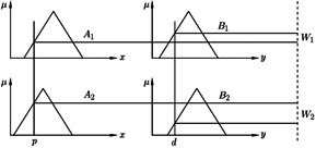
Takagi–Sugeno fuzzy inference system [20]
Then, the output of the fuzzy inference system is defined as
| (9) |
A typical equivalent ANFIS architecture is shown in Fig. 2.
Fig. 2.
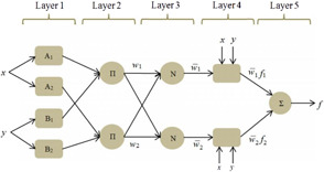
ANFIS architecture with five layers [21]
Five different layers of this structure are explained as follows. The membership values for inputs are determined in layer 1 based on the selected type of membership function. The incoming signals from the previous layer are multiplied and the firing strength of each rule is calculated in layer 2. Then in layer 3, the normalised firing strength of each rule is computed. The contribution of each rule in the model output is obtained in layer 4 based on Takagi–Sugeno rules ( as presented in (7) and (8)). Finally, in layer 5, the weighted global output of the system is calculated using (9) [20].
4.3.2 ANFIS learning process
There are two kinds of parameters (premise and consequent) in the ANFIS structure that should be modified using a learning process. Premise parameters are the coefficients of membership functions and their number varies based on the considered type and number of membership functions. Consequent parameters are coefficients of Takagi–Sugeno rules that are presented in (7) and (8).
The hybrid learning method is used for the training process. This method utilises two approaches, gradient descent and least square. In the feed forward pass, the consequent parameters are updated using the least square method. Then, in the backward pass, the difference between the output data and the ANFIS output (error) is used to update premise parameters using the gradient descent method.
4.4 Control strategy
The data obtained from the GA is used as the input for ANFIS. Then, the premise and consequent parameters are obtained from the ANFIS training process. These parameters are then used to build the Takagi–Sugeno fuzzy system. In the HCV epidemiological dynamics, the state variables are the input and the three optimal control signals are the output of the fuzzy system. This system is utilised as the controller in this study for the HCV treatment. It should be mentioned that a high number of inputs for the ANFIS, drastically increases the number of parameters that should be trained. To address this issue, only exposed (E) and acute infected (I) compartments are considered as inputs of the ANFIS. Fig. 3 illustrates a schematic diagram of the employed control strategy in the present work.
Fig. 3.
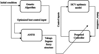
Schematic diagram of the control strategy
5 Result and discussion
In this section, the proposed OANF control strategy is evaluated in the HCV epidemic control in a population by performing some simulations. Three optimal control signals obtained using the ANFIS are implemented to minimise the proposed objective function (J) based on (6). Parameter values of the HCV epidemiological model and coefficients of the objective function (6) are adjusted and listed in Tables 4 and 5, respectively.
Table 4.
| Parameter | Value (1/day) | |
|---|---|---|
|
|
0.02 | |
|
|
0.01 | |
|
|
0.9 | |
|
|
10 | |
|
|
0.00024 | |
|
|
0.6 | |
|
|
0.5 | |
|
|
0.5 | |
|
|
0.15 | |
|
|
0.05 | |
|
|
0.23 | |
|
|
1 | |
|
|
0.13 | |
|
|
0.3 |
Table 5.
Objective function coefficients
| Parameter | Value (1/day) | |
|---|---|---|
|
|
100 | |
|
|
120 | |
|
|
110 | |
|
|
0.1 | |
|
|
0.5 | |
|
|
0.5 |
The screening rate (u 1), drug efficacy in the acute‐infected compartment (u 2), and drug efficacy in the chronic‐infected compartment (u 3) are considered as the normalised control inputs that should be in the range of [0, 1].
5.1 Results for the first initial condition
The initial conditions of different states are considered to be S = 360, E = 200, I = 200, T = 40, and V = 210. The response of the HCV epidemiological system during 120 days is shown in Fig. 4. As seen, in the case of no control signal (u 1 = u 2 = u 3 = 0), after a time period a large number of individuals are infected and transmitted to the acute‐infected (I) compartment. In this case (no control), the final values of state variables after 120 days are S = 20, E = 20, I = 2085, T = 0, and V = 30. However, using the proposed OANF control strategy, the final values of different states after the period of 120 days become S = 1432, E = 140, I = 146, T = 327, and V = 110, as observed in Fig. 4. Accordingly, the populations of the susceptible (S) and treated (T) compartments increase considerably in comparison with the case of no control input. Moreover, the susceptible (S) and treated (T) populations are higher than the exposed (E), acute‐infected (I), and chronic‐infected (V) populations in the presence of OANF control strategy.
Fig. 4.
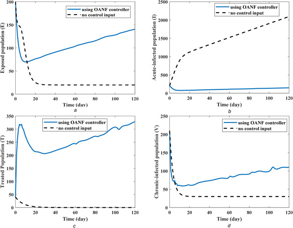
State values in the presence and absence of the proposed OANF control strategy
(a) Exposed population, (b) Acute‐infected population, (c) Treated population, (d) Chronic‐infected population
Due to (1), the dynamics of the total population (N) is obtained by summation of all compartments’ dynamics in (2) as
| (10) |
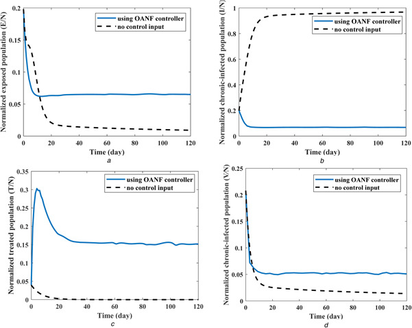
Accordingly, the change rate of the total population (N) depends on the recruitment rate (λ) and death rate (μ). In other words, an increase of the recruitment rate and decrease of the death rate will increase the total population variation . Based on the considered values for these two parameters (λ and μ) in Table 4, total population increases and reaches 2155 individuals from the initial population of 1010 people. Due to this increase, the population of all compartments (five state variables) is normalised with respect to the instant total population (N(t)) and represented in Fig. 5 during 120 days of treatment.
Fig. 5.
Normalised values of four state variables (compartment populations) with and without OANF control strategy
(a) Normalised exposed population, (b) Normalised acute‐infected population, (c) Normalised treated population, (d) Normalised chronic‐infected population
Initial normalised values of different states used in previous results are S = 0.356, E = 0.198, I = 0.198, T = 0.040 and V = 0.208. For the case of no control input, the normalised state variables converge to these final values: S = 0.009, E = 0.009, I = 0.968, T = 0 and V = 0.014, as seen in Fig. 5. As mentioned previously, about 97% of the total population transmits to the acute‐infected compartment (I) after 120 days, in the absence of medical intervention (control inputs). By employing the proposed OANF controller, the final values of different HCV compartments are obtained as S = 0.664, E = 0.065, I = 0.068, T = 0.152 and V = 0.051. In this case, the population of inappropriate compartments (E + I + V) has 61% of the total population (N) at the first day, which decreases to 19% of the total population (N) after 120 days of using this control strategy.
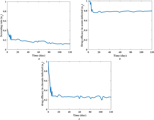
The screening rate (u 1), drug efficacy in the acute‐infected compartment (u 2), and drug efficacy in the chronic‐infected compartment (u 3) as the control inputs are illustrated in Fig. 6. Note that higher control inputs are implemented at the first days because the normalised exposed (E/N), acute infected (I/N) and chronic infected (V/N) populations are higher at the first days in comparison with their values after 10 days of epidemic control. Fig. 7 shows the value of the objective function (6) during 120 days of a process for the proposed OANF controller and a previous optimal controller [12]. In that optimal control strategy [12], constant control inputs are considered as u 1 = 0, u 2 = u 3 = 1.
Fig. 6.
Control inputs during 120 days of the HCV epidemic control using the OANF strategy
(a) Screening rate (u 1), (b) Drug efficacy for acute‐infected (u 2), (c) Drug efficacy for chronic‐infected (u 3)
Fig. 7.
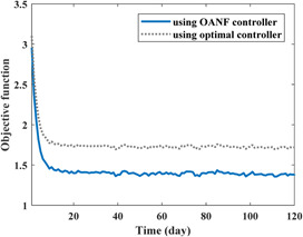
Value of the objective function for 120 days by employing the proposed OANF strategy and the previous optimal strategy [12]
At the first days of HCV treatment, the values of control inputs obtained by the suggested OANF strategy (Fig. 6) are approximately close to the ones (u 1 = 0, u 2 = u 3 = 1) used in the optimal strategy [12]. Accordingly, the value of the objective function using the proposed OANF and optimal strategies are close to each other in Fig. 7 at initial days. However, after a period of time (about 10 days) that lower control rates are commanded by the proposed OANF strategy (Fig. 6), the objective function value is smaller for the OANF controller in comparison with the one for the optimal controller. This means that the constant extremum control inputs (u 1 = 0, u 2 = u 3 = 1) are not required after the first period of the HCV epidemic control (after 10 days). The time integral of the objective function for the optimal control method is ; however, using the OANF control method this value decreases to . Therefore, one can conclude that the proposed OANF control strategy intelligently obtained required time‐varying control inputs unlike the previous optimal controller [12] that suggested constant inputs.
5.2 Results for some different parameters with new initial conditions
Based on the sensitivity analysis [12], λ and β 1 have the highest sensitivity in comparison with the other parameters. Thus, in order to investigate the effectiveness of the proposed strategy, some new values are considered for the state conditions and mentioned parameters. Initial conditions for different compartments are S = 420, E = 250, I = 300, T = 80 and V = 250. For the first case, recruitment rate (λ) is considered to be 15 which was 10 in the previous simulations. Fig. 8 depicts the population of the acute‐infected compartment (I) during 60 days of treatment. The initial population of 300 (0.23 of the total population) has reached 2055 (0.95 of total population) after 60 days in the absence of control inputs. However, employing the proposed controller, the population will become 146 (0.067 of the total population).
Fig. 8.
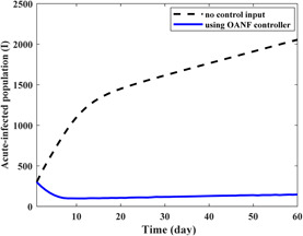
Population of the acute‐infected compartment in the presence and absence of the proposed OANF control strategy for λ = 15 for 60 days
For the second case, 50% increase is considered for the recruitment rate (λ) and the transmission rate of acutely infected population . Therefore, λ is changed to 15 and is changed to 0.7. The corresponding simulation results are presented in Fig. 9. The initial population of 300 for acute‐infected individuals (I) reaches 2055 and 146 in the absence and presence of the proposed strategy, respectively.
Fig. 9.
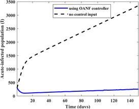
Population of the acute‐infected compartment in the presence and absence of the proposed OANF control strategy for λ = 15 and β1 = 0.7 for 150 days
Based on the previous results and discussions, it could be concluded that the HCV epidemic model with different parameter values which represent different societies could be controlled using the proposed strategy. Moreover, this control method can be employed for other diseases and epidemics.
5.3 Statistical analysis of methods
In this section, statistical analysis is presented to compare results between the proposed methods with previous one [12]. In statistics, one‐way analysis of variance (ANOVA‐1) is commonly used to compare means of two or more levels. These levels correspond to different groups or conditions [23].
In the analysis for this study, two methods (OANF and optimal controller [12]) are considered as two groups and the cost function (6) is supposed to be the dependent variable. Results of ANOVA‐1 analysis are presented in Table 6.
Table 6.
Result of ANOVA‐1 analysis
| Sum of squares | d.f. | Mean square | F | Sig. | |
|---|---|---|---|---|---|
| between groups | 7.815 | 1 | 7.815 | 10.357 | 0.001 |
| within groups | 223.355 | 296 | 0.755 | — | — |
| total | 231.170 | 297 | — | — | — |
The d.f. is defined as degrees of freedom. Some of the squares exhibit variability between groups and within groups [24]. F ratio represents the variance between the groups divided by the variance within the groups [23]. The last column of Table 6 represents the significance value (sig.) which is the main parameter for analysis. For the case that Sig. value is >0.05, there the null hypothesis will be confirmed. On the other hand, if this value is ≤0.05, the null hypothesis will be rejected and there is a significant difference among the mean score on the dependent variable for different groups [23].
The results of Table 6 show that the value of the Sig. which is equal to 0.001 and is <0.05. So, it could be concluded that there is a significant difference in the mean scores of the cost function (6) between the two mentioned methods.
6 Conclusion
An OANF controller was designed to control the HCV spread in a population with different compartments. GA was employed to obtain the optimal control inputs based on the values of the objective function. Output results of GA were used as the training data for the proposed ANFIS. The output of the ANFIS is a Takagi–Sugeno fuzzy structure used as an intelligent controller for the HCV epidemic. Numerical results of this control strategy showed that the population of the acute‐infected compartment decreased from 20% of the total population to <7% during 120 days of the treatment. However, in the absence of control inputs, the acute‐infected population increased and reached 97% of the total population at the end of 120 days. Moreover, using the proposed strategy, the value of the objective function decreased 19% in comparison with a previous optimal control method by utilising smaller control inputs. Statistical analysis (ANOVA‐1) shows that there is a significant difference between the results of the proposed method and the previous one. In addition, results with different values of model parameters illustrate that the proposed method could be effective for different societies.
7 References
- 1.‘Hepatitis C ’: Available at http://www.who.int/mediacentre/factsheets/fs164/en/, accessed 1 November 2017
- 2. Shen M., Xiao Y., and Zhou W. et al.: ‘Global dynamics and applications of an epidemiological model for hepatitis C virus transmission in China’, Discret. Dyn. Nat. Soc., 2015, 2015, pp. 1–13 [Google Scholar]
- 3. Martcheva M., and Castillo‐Chavez C.: ‘Diseases with chronic stage in a population with varying size’, Math. Biosci., 2003, 182, pp. 1–25 [DOI] [PubMed] [Google Scholar]
- 4. Zhang S., and Zhou Y.: ‘Dynamics and application of an epidemiological model for hepatitis C’, Math. Comput. Model., 2012, 56, pp. 36–42 [Google Scholar]
- 5. Hullegie S.J., Van Den Berk G.E.L., and Leyten E.M.S. et al.: ‘Acute hepatitis C in the Netherlands: characteristics of the epidemic in 2014’, Clin. Microbiol. Infect., 2016, 22, (2), p. pp. 209.e1–2209.e3 [DOI] [PubMed] [Google Scholar]
- 6. Yuan J., and Yang Z.: ‘Global dynamics of an SEI model with acute and chronic stages’, J. Comput. Appl. Math., 2008, 213, (2003), pp. 465–476 [Google Scholar]
- 7. Shi R., and Cui Y.: ‘Global analysis of a mathematical model for hepatitis C virus transmissions’, Virus Res., 2016, 217, pp. 8–17 [DOI] [PubMed] [Google Scholar]
- 8. Chen J., and Li F.: ‘Development of hepatitis C virus vaccine using hepatitis B core antigen as immuno‐carrier’, World J. Gastroenterol., 2006, 12, (48), pp. 7774–7778 [DOI] [PMC free article] [PubMed] [Google Scholar]
- 9. Zhang S., and Xu X.: ‘Dynamic analysis and optimal control for a model of hepatitis C with treatment’, Commun. Nonlinear Sci. Numer. Simul., 2017, 46, pp. 14–25 [Google Scholar]
- 10. Cai L., and Li X.: ‘A note on global stability of an SEI epidemic model with acute and chronic stages’, Appl. Math. Comput., 2008, 196, pp. 923–930 [Google Scholar]
- 11. Oare O.K.: ‘Impact and optimal control of movement on a multipatch hepatitis C virus model’, TWMS J. Pure Appl. Math., 2014, 5, (1), pp. 80–95 [Google Scholar]
- 12. Okosun K.O., and Makinde O.D.: ‘Optimal control analysis of hepatitis C virus with acute and chronic stages in the presence of treatment and infected immigrants’, Int. J. Biomath., 2014, 7, (2), pp. 1–23 [Google Scholar]
- 13. Ainea N., Massawe E.S., and Makinde O.D. et al.: ‘Mathematical analysis of control strategies of HCV in a community with inflow of infected immigrants’, Sci. Res. publishing, 2015, 5, pp. 1–13 [Google Scholar]
- 14. Abdelrazec A., Bélair J., and Shan C. et al.: ‘Modeling the spread and control of dengue with limited public health resources’, Math. Biosci., 2016, 271, pp. 136–145 [DOI] [PubMed] [Google Scholar]
- 15. Sharifi M., and Moradi H.: ‘Nonlinear robust adaptive sliding mode control of influenza epidemic in the presence of uncertainty’, J. Process Control, 2017, 56, pp. 48–57 [Google Scholar]
- 16. Melanie M.: ‘An introduction to genetic algorithms’ (A Bradford Book/The MIT Press, Massachusetts, 1998, 1st edn.) [Google Scholar]
- 17. Haupt R.L., and Haupt S.E.: ‘Practical genetic algorithms’ (John Wiley & Sons, New York, 2004, 2nd edn.) [Google Scholar]
- 18. Mosaad M.I., and Salem F.: ‘LFC based adaptive PID controller using ANN and ANFIS techniques’, J. Electr. Syst. Inf. Technol., 2014, 1, (3), pp. 212–222 [Google Scholar]
- 19. Jang J.R.: ‘ANFIS: adaptive network based fuzzy inference system’, IEEE Trans. Syst. Man. Cybern., 1993, 23, (3), pp. 665–685 [Google Scholar]
- 20. Bachi I.O., Abdulrazzaq N., and He Z.: ‘Neuro fuzzy model for predicting the dynamic characteristics of beams’, Acta Mech. Solida Sin., 2014, 27, (1), pp. 85–96 [Google Scholar]
- 21. Vatankhah R., Broushaki M., and Alasty A.: ‘Adaptive optimal multi‐critic based neuro‐fuzzy control of MIMO human musculoskeletal arm model’, Neurocomputing, 2016, 173, pp. 1529–1537 [Google Scholar]
- 22. Vatankhah R., and Asemani M.H.: ‘Output feedback control of piezoelectrically actuated non‐classical micro‐beams using TS fuzzy model’, J. Franklin. Inst., 2017, 354, (2), pp. 1042–1065 [Google Scholar]
- 23. Pallant J.: ‘SPSS survival manual’ (McGraw‐Hill, Maidenhead, 2013, 5th edn.) [Google Scholar]
- 24. Hatch E., and Farhadi H.: ‘Research design and statistics’ (Rahnoma Publication, Tehran, 2011, 1st edn.) [Google Scholar]


