Multispecies coalescent and its applications to infer species phylogenies and cross-species gene flow

Abstract

Multispecies coalescent (MSC) is the extension of the single-population coalescent model to multiple species. It integrates the phylogenetic process of species divergences and the population genetic process of coalescent, and provides a powerful framework for a number of inference problems using genomic sequence data from multiple species, including estimation of species divergence times and population sizes, estimation of species trees accommodating discordant gene trees, inference of cross-species gene flow and species delimitation. In this review, we introduce the major features of the MSC model, discuss full-likelihood and heuristic methods of species tree estimation and summarize recent methodological advances in inference of cross-species gene flow. We discuss the statistical and computational challenges in the field and research directions where breakthroughs may be likely in the next few years.

INTRODUCTION

Developed in the 1980s, the coalescent is a stochastic process that describes the genealogical history of a sample of DNA sequences taken from a population [1–3]. Whereas traditional population genetic models of drift and mutation describe changes in allele frequencies over generations in the population, the coalescent focuses on the sample and traces the genealogical history of lineage joining of the sampled sequences backwards in time. The coalescent model is in particular suited to inference using genetic sequence data [4–7].

The multispecies coalescent (MSC) is an extension of the single-population coalescent to the case of multiple species [8]. It integrates the process of species divergences and the within-population process of drift and mutation. Placing the coalescent in the context of a species phylogeny makes it possible to use the ever-increasing genomic sequence data from multiple species to address a number of important biological questions, and in the past two decades, the MSC has emerged as the natural framework for such inferences. These include estimation of population parameters (such as species divergence times, population sizes for extant species and extinct ancestors and rates of cross-species gene flow), estimation of species phylogeny accommodating heterogeneous gene genealogies across the genome and delineation of species boundaries (species delimitation) [9–12]. In molecular phylogenetics, incorporation of the MSC to accommodate the so-called gene-tree–species-tree conflicts has been heralded as a ‘paradigm shift’ [13]. Stochastic fluctuation in genealogical history of sequences across the genome, when accommodated in the model, is not a ‘conflict’ or ‘problem’, but rather a source of information for important evolutionary parameters such as ancestral population sizes [14–16] and rates of cross-species gene flow [17,18].

The past decade has seen exciting advancements in the implementation and extension of the MSC model for inference using genomic sequence data. The data we consider in this review are sequence alignments at hundreds or thousands of loci, with the different loci having independent coalescent histories while all sites in the sequence at the same locus share the same history. Ideal data for such analysis are short segments sampled from the genome that are far apart [16]. While we use the term gene or locus, the data should ideally be non-coding DNA, although exonic data have been successfully used in such analyses [19,20]. We describe the major features of the MSC model (in particular, the probability distribution of gene trees and coalescent times), and discuss its applications in two major areas: the estimation of the species phylogeny and the inference of cross-species gene flow. We focus on full-likelihood methods (maximum likelihood or ML and Bayesian inference), as they have the best statistical properties, but include heuristic methods based on summaries of the data in our discussion. Several comprehensive reviews on heuristic methods have been published [9,10,21–23]. We review recent advances in using the MSC model to infer ancient gene flow, including models of continuous migration (the so-called isolation-with-migration model) and the introgression/hybridization models. We end the paper with a discussion of the challenges and perspectives in the field. Our focus in this review is on MSC-based analyses of multilocus sequence data, and we do not consider population genetics methods that use summary statistics such as allele frequencies and single nucleotide polymorphisms (SNPs) to infer demographic processes including population structure and admixture [24,25].

MULTISPECIES COALESCENT

Fisher-Wright model and the coalescent

The Fisher-Wright model [26,27] in population genetics describes the biological process of reproduction and drift in an idealized population of constant size, with non-overlapping generations, random mating and no population structure or selection (Fig. 1(a)). Individuals of the next generation are generated by random sampling of gametes from the current population: the frequencies of alleles at a locus (say, A and a for two alleles) in the next generation are generated by binomial sampling given the allele frequencies in the current generation.

Figure 1.

The Fisher-Wright model for a diploid population of N individuals or 2N = 20 sequences, with n = 5 sequences sampled at random from the present generation. The coalescent focuses on the genealogical relationships among the sampled sequences (in blue). Coalescent time T_i (during which there are i lineages in the sample) is in generations.

The coalescent model describes the same process of reproduction and drift, with the focus on the sample of sequences and with time running backwards (Fig. 1(b)) [1]. When we trace the genealogical history of the sample backwards in time, lineages join or coalesce when we reach their common ancestors. While the forward Fisher-Wright model and backward coalescent model are two characterizations of the same process, the coalescent approach of focusing on the sample offers major advantages for many inference problems using genetic sequence data. For example, coalescent simulation of the genealogy of the sample is often far more efficient than forward simulation tracking the whole population. The basic coalescent model has been extended to accommodate demographic changes, recombination, population subdivision and selection [5,7]. Here we focus on the basic coalescent and on the probability distribution of gene tree topologies and coalescent times generated by the process.

Consider first n = 2 sequences sampled from a diploid population of size N. With random mating assumed in the Fisher-Wright model, sequences pick parents at random when we trace the genealogical history of the sample to the previous generation. As there are 2N parental sequences to choose from, the probability that the two sequences pick the same parent (that is, they coalesce) in the previous generation is 1/(2N). In other words, coalescent occurs as a Poisson process at the rate of 1/(2N), faster in smaller populations, and the coalescent time (the waiting time until the two sequences find their common ancestor) has a geometric distribution with the mean of 2N generations. Thus, two sequences sampled at random are on average separated by 2N × 2 generations or θ = 4Nμ mutations per site, where μ is the mutation rate per site per generation. Parameter θ, known as the population size parameter, is the average distance between two sequences sampled at random from the population. It is also known as heterozygosity and can vary hugely even between close species. Typical values include for humans [28] and 0.1%–5% for Heliconius butterflies [29].

In analysis of sequence data, it is convenient to measure time by the mutational distance so that one time unit is the expected time to accumulate one mutation per site. With this time unit, the coalescent waiting time for two sequences (t₂) is approximately exponential with the mean θ/2, with density

(1)

If there are n > 2 sequences in the sample, there will be pairs and each pair coalesce at the rate of 2/θ, with the total rate . The time until the next coalescent event has an exponential distribution with mean

When a coalescent occurs, each of the pairs has the same probability to join. The number of lineages is then reduced from n to n − 1, and the process repeats, until the most recent common ancestor (MRCA) is reached (Fig. 1(b)).

The n − 1 successive coalescent events generate a genealogical tree (G) of the sequences in the sample. This is a rooted tree with the internal nodes ranked by age, and is called the ranked tree or labelled history [30] (Fig. 1(b)). The number of possible labelled histories for a sample of size n is

and each of them occurs with equal probability, f(G) = 1/H_n. Furthermore, the n − 1 coalescent times are independent exponential variables, with means

The joint probability density of the gene tree and coalescent times is thus

(2)

Multispecies coalescent: basic features

The extension of the single-population coalescent to multiple species has been called the interspecific coalescent [31] or censored coalescent [8], and is now commonly known as the multispecies coalescent [32]. Suppose that there are s species, which are related through a species phylogeny. Instead of a single parameter θ, the model now involves two sets of parameters: s − 1 species divergence times (τs) and 2s − 1 population size parameters (θs), with a total of 3s − 2 parameters (Fig. 2). Both the τ and θ are measured in the expected number of mutations per site.

Figure 2.

A species tree for three species (A, B and C) showing parameters in the MSC model, and the four possible coalescent histories for a locus with one sequence from each species, with probabilities , where is the probability that sequences b and c do not coalesce in species BC. Note that the first two histories correspond to the same rooted gene tree G₁, and there are three gene trees: G₁, G₂ and G₃.

Given the species tree, coalescent events occur independently in different populations, with the coalescent rate (2/θ) given by the population size. When we trace the history of the sequences at a locus backwards in time and reach a speciation event, the coalescent process and rate are reset, because of the change in population size and because of sequences coming from the sibling species. For example, in Fig. 3, sequences c₁ and c₂ coalesce at the rate 2/θ_C in species C. When they enter species BC at time τ_BC, the coalescent rate (for each pair) is reset to 2/θ_BC and the number of lineages becomes 3. Furthermore, we assume that gene trees at different loci are independent. One important feature of the MSC model is that the divergence time between sequences from two species must be greater than the species divergence time: sequences split before species or equivalently the gene tree fits inside the species tree. This intrinsic constraint between the species tree and the gene trees is the source of computational challenges in Bayesian implementations of the MSC model.

Figure 3.

A species tree for three species, (A, (B, C)), with a gene tree for five sequences at a locus to illustrate the MSC density of the gene tree with coalescent times.

There are two important probability distributions under the MSC model: the (marginal) probabilities of gene tree topologies [21,33,34] and the joint distribution of the gene tree topology and coalescent times [8]. The former is useful for two-step methods of species tree estimation, which use reconstructed gene tree topologies as data, while the latter is used in full-likelihood methods, which use information in gene tree branch lengths (coalescent times) as well.

Probabilities of gene tree topologies

Under the MSC model, the gene tree topologies and coalescent times have a joint probability distribution given the species tree and parameters. For small species trees, it is easy to derive the marginal probability of gene tree topologies [2,33,35]. This line of work typically assumes one sequence sampled per species at every locus, so that there is no coalescent in modern species at the tips of the species tree. The case of three species is considered in [2]. Let the three species be A, B and C, with the phylogeny S = (A, (B, C)) (Fig. 2). Let the divergence times be and the population sizes be . Suppose that three sequences are sampled from the three species (a, b and c). There are three possible gene tree topologies: G₁ = (a, (b, c)) matches the species tree, while G₂ = (b, (c, a)) and G₃ = (c, (a, b)) are the mismatching gene trees.

When we trace the genealogy of the three sequences, sequences b and c may coalesce in population BC as a Poisson event at the rate of 2/θ_BC just as in the single-population coalescent. Note that the probability that a Poisson event of rate λ does not occur in a time interval t is . Thus, the probability that sequences b and c do not coalesce in population BC or over the time interval Δτ = τ_ABC − τ_BC is

(3)

Here Δτ/(θ_BC/2) is known as the internal branch length in coalescent units—one coalescent unit in population BC is 2N_BC generations or θ_BC/2 mutations per site. If b and c coalesce in population BC, the gene tree must be G₁. Otherwise, all three sequences enter species ABC and coalesce in random order so that the three gene trees occur with equal probability. Thus, the probabilities for the three gene trees (G₁, G₂, G₃) are

(4)

For certain species trees and parameter values, a mismatching gene tree may be more probable than the matching gene tree. The species tree is then said to be in the anomaly zone [33,34]. The anomaly zone does not exist for species trees of three species—as in equation (4), but can occur for asymmetrical species trees of four species, and for any species tree of five or more species [34].

Consider the asymmetrical species tree for four species S = (A, (B, (C, D))) of Fig. 4, and suppose that the three divergence times are very close, with τ_ABCD ≈ τ_BCD ≈ τ_CD. Then all three coalescent events for the four sequences (a, b, c and d) will most likely occur in the root population ABCD, so that the labelled histories will have nearly equal probability . There are 15 possible rooted gene trees, 12 asymmetrical and 3 symmetrical. Each symmetrical gene tree (e.g. G₂ in Fig. 4) corresponds to two labelled histories (G_2a and G_2b in Fig. 4), so that its probability is . Each of the 12 asymmetrical gene trees (e.g. G₁ in Fig. 4) is compatible with only one labelled history, with probability . Thus, . When the divergence times (τs) are unequal but the internal branches are short enough, it is possible for the symmetrical mismatching gene tree G₂ to have a higher probability than the matching asymmetrical gene tree G₁, in which case the species tree is in the anomaly zone.

Figure 4.

Asymmetrical species tree for four species A, B, C and D, and three labelled histories (G₁, G_2a, G_2b) for a locus with one sequence from each species. Here G₁ matches the species tree, while G_2a and G_2b are distinct labelled histories sharing the same topology ((a, b), (c, d)), which is different from the species tree.

If the species tree is in the anomaly zone, the simple majority-vote approach of using the most commonly observed gene tree as the estimate of the species tree is statistically inconsistent: the more gene trees there are, the more certain that the species-tree estimate will be incorrect. Note that the existence of the anomaly zone is not an intrinsic difficulty for species tree estimation; it instead highlights the importance of adopting a proper statistical inference framework. Full-likelihood methods are consistent for all species trees both inside and outside the anomaly zone, as they accommodate the probability distribution of the gene trees under the MSC appropriately. The discussion of the anomaly zone typically assumes true gene trees and ignores phylogenetic reconstruction errors in estimated gene trees. There have been only a handful of empirical examples of the anomaly zone, in African Anopheles mosquitoes [20], skinks [36], flightless birds [37] and gibbons [19].

The probabilities of gene tree topologies can be used to calculate the likelihood function for estimating the species tree using (reconstructed) gene trees as input data, as in the stells program [38]. However, popular heuristic methods such as mp-est [39] and astral [40] do not use this theory and are instead based on species triplets or quartets. Furthermore, calculation of the probabilities of gene tree topologies, which involves summing over all coalescent histories that are compatible with each gene tree, becomes expensive when the number of species increases [21].

Joint probability distribution of gene trees and coalescent times

While the marginal probability of the gene tree topology may be challenging to compute, it is straightforward to derive the joint distribution of gene tree topologies and coalescent times. The general form, for an arbitrary species tree and an arbitrary number of sequences, is given in [8].

The joint density of gene trees and coalescent times is a product over the populations on the species tree, and as a result, we focus on the contribution from one population. A population is represented by a branch on the species tree (say XY) or by the daughter node of the branch (say X). Let τ_X and τ_Y be node ages or divergence times, and θ_X be the population size. Suppose that m sequences enter the population at time τ_X and l sequences leave the population at time τ_Y, with 1 ≤ l ≤ m. For example, in the gene tree of Fig. 3, m = 3 lineages enter population BC while l = 2 lineages leave it. Unlike the single-population coalescent, under the MSC, lineages entering a population do not necessarily find their common ancestor in that population, and the coalescent process may be ‘censored’ [8]. Note that if X is the root of the species tree, l must be 1.

The MSC density for the part of the gene tree residing in population XY is the product of three components. The first is the joint density of the m − l independent exponential coalescent waiting times . The second component is for the gene tree topology in XY, and is a product of m − l probabilities, each being the probability, , of choosing two out of i lineages to join, for i = m, m − 1, …, l + 1. These two components are the same as in the single-population coalescent. The third component is the probability that no coalescent events occur in the last time interval before reaching τ_Y. Multiplying the three components, we obtain the MSC density of the gene tree in XY as

(5)

For example, the contribution of species BC to the MSC density of the gene tree in Fig. 3 is

(6)

As coalescent processes in different populations operate independently, the MSC density for the whole gene tree at a locus is the product of the contributions across all populations. For the gene tree of Fig. 3, this is

(7)

The four pairs of brackets correspond to species A, C, BC and ABC, respectively. Coalescence is not possible in species B as only one sequence is sampled from that species.

With multiple loci in the data, the joint MSC density of the gene trees is a product across all loci, because the genealogical histories at different loci are assumed to be independent. The formulation allows the loci to have different sampling configurations. For example, the number of sequences from each species may vary among loci and some species may be missing at some loci.

SPECIES TREE INFERENCE UNDER THE MSC

Species-tree–gene-tree conflicts

The gene tree representing the coalescent history of the sequences at a locus may not match the species tree. Such a discordance may occur because when we trace the history of the sample backwards in time, sequences from different species may not coalesce as soon as they reach the most recent common ancestor on the species tree but instead coalesce in more ancient ancestors (e.g. gene trees G_1b, G₂, G₃ in Fig. 2). This delayed coalescence or deep coalescence is also known as incomplete lineage sorting. While several biological processes, including gene duplication followed by gene loss or horizontal gene transfer [41,42], can cause the gene tree to differ from the species tree as well, deep coalescence is more fundamental because coalescent is simply biological reproduction and drift and thus may affect every species. Deep coalescence is more common when multiple species arise through a rapid succession of speciation events, resulting in very short internal branches on the species tree relative to the coalescent waiting time (note that φ in equation (3) is greater for smaller Δτ and larger θ_BC). The existence of the anomaly zone is an extreme case of deep coalescence. Deep coalescence is related to how short the internal branches are, rather than how deep they are on the species tree, and may thus occur in both shallow and deep species trees [43].

Full-likelihood methods

ML methods [44,45] and Bayesian inference [46–49] use the joint distribution of gene trees and coalescent times [8] and operate on multilocus sequence data directly. Let the sequence data be , where X_j is the alignment of n_j sequences at the jth locus for j = 1, 2, …, L. Let S be the species tree, and let be the vector of parameters, including species divergence times (), population sizes () and parameters in the mutation model (η). The likelihood of the sequence data given the MSC model has the form

(8)

where is the phylogenetic likelihood given the gene tree G_j and branch lengths at locus j [50], while is the MSC density of the gene tree described above [8]. As the genealogical histories at different loci are independent, the likelihood of the sequence data is a product across all loci. The summation in equation (8) is over all possible gene tree topologies for the sequences, and the integral is n_j − 1 dimensional, over the n_j − 1 coalescent times on each gene tree. The gene trees and coalescent times are not observed, and the likelihood function averages over them, accommodating their uncertainties.

The species tree S and the MSC parameters Θ can be estimated using ML by maximizing equation (8). Both the phylogenetic likelihood and MSC density are straightforward to calculate, but averaging over all the possible gene tree topologies and coalescent times at each locus is computationally infeasible except for small data sets. The only ML implementation available is the 3s program [44,45], which enumerates the gene trees and uses numerical integration (Gaussian quadrature) to calculate the integrals. Although limited to three species and three sequences per locus, 3s can handle tens of thousands of loci.

With more than three species, the Bayesian method has a computational advantage over ML, with the Markov chain Monte Carlo (MCMC) algorithm averaging over the gene trees and coalescent times. We assign prior distributions to the species tree and model parameters. For example, the species tree can be assigned a uniform prior over all rooted trees, while the population-size parameters (θs) can be assigned gamma or inverse-gamma priors. The inverse-gamma priors for the θ are conjugate (so that both the prior and posterior for the θ are inverse gamma), allowing the θ to be integrated out analytically [51], which helps with MCMC mixing. The age of the species-tree root can be assigned a gamma or inverse-gamma prior, while the other node ages can be constructed using a Dirichlet distribution [52]. The MCMC algorithm samples from the joint posterior distribution of the species tree, the MSC parameters and the gene trees at all loci

(9)

In particular, the samples of (S, Θ) generated by the algorithm are from the marginal posterior , and the frequency at which a species tree is visited is an estimate of its posterior probability. In this way, MCMC averages out the gene trees and coalescent times numerically.

The first implementation of the Bayesian approach is the program best [53]. This uses the samples of gene trees with branch lengths produced by MrBayes [54] and applies an importance-sampling correction because MrBayes does not assume that the gene trees are distributed according to the MSC density. This strategy does not work well, as the species tree and the gene trees place tight constraints on each other in the MSC model. Currently, two Bayesian programs under the MSC are in common use: *beast [46] and bpp [47–49], both of which explicitly use the MSC model. The algorithm in bpp for species tree inference goes through several proposal steps in each MCMC iteration, as follows.

1. Update the coalescent times on the gene tree at each locus j.

2. Update the gene tree topology G_j at each locus j through a subtree-pruning-and-regrafting (SPR) algorithm.

3. Update the population sizes (θs).

4. Update the species divergence times (τs).

5. Update the species tree topology S through a nearest-neighbor interchange (NNI) or SPR move, which may change the gene trees to avoid conflicts.

6. Use a multiplier to rescale all node ages on the species tree and on all gene trees.

Perhaps the greatest challenge in such MCMC algorithms comes from the constraint between the species tree and the gene trees. Consider step 4 for changing species divergence time τ_AB, the age of the ancestral node for two sister species/clades A and B. Let t_ab be the sequence divergence time for two sequences from A and B. Then τ_AB < t_ab. If the dataset includes thousands of loci and many sequences from A and B at each locus, the smallest of t_ab among all loci may be almost identical to the current τ_AB. Then, when we use a sliding window to change τ_AB, the window size will have a width near zero, and the MCMC is virtually stuck. A ‘rubber-band’ algorithm was proposed in [8], which changes τ and the affected node ages on gene trees jointly. Similarly, in step 5, it is very inefficient to change the species tree when all gene trees are fixed. A breakthrough was to make coordinated changes to the gene trees when an NNI algorithm is used to change the species tree [47]. The algorithm has since been extended to SPR [48,55] and ported to *beast as well [55,56]. Those improvements have pushed the limit of datasets that can be analyzed using Bayesian MCMC programs from ∼100 to ∼10 000 loci [19,20].

Heuristic or summary methods

Many heuristic methods for species tree estimation have been developed, which use summaries of the data rather than the original mutlilocus sequence alignments. For extensive reviews, see [9,10,22,23]. Here we mention four commonly used ones: mp-est [39], astral [40], NJ-st [57] and SVDQuartets [58].

MP-est [39] estimates triplet gene trees under the molecular clock (rate constancy among lineages), and then uses a composite likelihood function, treating the frequencies of the triplet gene trees as input data from a trinomial distribution (with probabilities given in equation (4)). A composite or pseudo-likelihood is constructed by multiplying those probabilities for all possible triplets, ignoring lack of independence among them. This composite likelihood is maximized to estimate the species tree.

Astral [40] uses a phylogenetic method to infer unrooted gene trees, and extracts the quartets from them. It then finds the species tree that is most compatible with the quartets in the set. A procedure has also been developed to attach local support values for nodes on the inferred species tree [59].

NJ-st [57] uses a distance method to estimate an unrooted species tree from a collection of unrooted gene trees. The species tree estimate is the neighbor-joining tree built from a distance matrix where the distance between two species is defined as the average number of internal nodes on the gene tree between the species.

All those three methods are two-step methods, treating estimated gene tree topologies as data. They are consistent, with the probability to recover the correct species tree approaching 1 when the number of gene trees increases. As discussed above, the anomaly zone does not exist for rooted triplets or equivalently for unrooted quartets. However, the argument for consistency is based on the assumption that the input gene trees are known without error. Phylogenetic reconstruction errors are known to affect the performance of two-step methods [60]. Furthermore, as those two-step methods use gene tree topologies but not branch lengths or coalescent times, they suffer from unidentifiability issues [9]. They can estimate the species tree topology but not all parameters in the MSC model.

Another summary method is called SVDQuartets [58]. This is a quartet method, designed for data of coalescent-independent sites, sites that have independent histories. Such sites are similar to SNPs but include constant sites as well. Genome sequencing projects do not generate such data. When the method is applied to multilocus sequence alignments, sites are pooled across loci, as in the concatenation method, so that the data are the counts of 256 (=4⁴) site patterns for the species quartet. Note that the site-pattern counts pooled across loci are summaries of the original multilocus alignments. When all sites have independent histories, the summation over gene trees and the integral over coalescent times under the MSC model (equation (8)) are analytically tractable [58,61]. Pooling sites across loci causes information loss and identifiability issues, so that the method is unable to identify all parameters in the MSC model even if the species tree topology is identifiable [9,62].

Some two-step methods use both gene tree topologies and branch lengths (coalescent times) [63]. However, those methods were found to have poorer performance than methods based on topologies alone [64,65]. This is because the methods ignore random sampling errors in branch-length estimates. It is easy to see that sampling errors in branch lengths may have a major impact on estimation of the species tree and the MSC parameters. For example, if two sequences from two species are identical at a locus so that the estimated coalescent time is t_ab = 0, the species divergence time τ_AB will be forced to be 0 as well (since τ_AB < t_ab), which may have a dramatic effect on species tree estimation. While coalescent times or branch lengths on gene trees contain much information [62], it is important to accommodate their uncertainties.

Comparison between full-likelihood and heuristic methods

Figure 5 shows results from a small simulation to illustrate the different performance of a full-likelihood method (bpp), two summary methods (astral and mp-est) and ML analysis of concatenated data. The species tree is challenging with short internal branches in both sets of simulations. Bpp recovered the true species tree with higher probability than the two summary methods and concatenation. For set 1, all four methods are consistent, with the probability of recovering the true species tree approaching 1 for every method when the number of loci increases. For set 2, the species tree is in the anomaly zone, and concatenation/ML is inconsistent, with the probability for the mismatching balanced tree approaching 1, while the other three methods are consistent. Note that the ML method applied to concatenated data assumes one tree and one set of divergence times for all loci and can be inconsistent [67].

Figure 5.

A simulation experiment to compare four methods of species tree estimation: ML analysis of concatenated data, , and . (a) Species tree used in the simulation. Two sets of parameter values are used: τ_ABCDO = 3θ, τ_ABCD = 1.25θ, τ_ABC = 1.125θ and τ_AB = θ in set 1, and τ_ABCDO = 3θ, τ_ABCD = 1.05θ, τ_ABC = 1.025θ and τ_AB = θ in set 2, with θ = 0.01. (b) and (c) Proportion of replicates in which the estimated species tree is the true tree (blue) or the mismatching tree S = (((A, B), (C, D)), O) (red). Data of multilocus alignments were simulated using the simulate option of [49] under the JC69 model [66], with one sequence sampled per species at each locus, and with a sequence length of 500 sites. The outgroup sequence (O) is used to root the tree by concatenation/ML and , but not used by or . The number of replicates is 100 for and 500 for the other methods.

Heuristic methods based on data summaries have a huge computational advantage over full-likelihood methods. For large datasets with hundreds or thousands of species and thousands of loci, they may be the only methods that are currently feasible computationally. Heuristic methods have poorer statistical performance than full-likelihood methods, and the difference can be large for challenging species trees with short internal branches [9,19,62,64,68]. As two-step methods typically ignore phylogenetic reconstruction errors in gene trees, their performance may suffer from uncertainties in the gene trees [60,64]: for those methods, species trees are only as good as the gene trees on which they are built [9,23].

An important strength of full-likelihood methods is that they can provide estimates of parameters in the MSC model when the species tree is fixed [16,56]. The MSC model for a species tree of s species has s − 1 divergence times (τs) and 2s − 1 population sizes (θs) (Fig. 2), all of which can be identified and estimated by full-likelihood methods using multilocus sequence data. In contrast, summary methods use only a portion of information in the data and are unable to identify all parameters in the model. For example, in the case of three species, the MSC model involves seven parameters (two τ and five θ), but there are only two distinct frequencies of gene trees (equation (4)), so that two-step methods using gene tree topologies alone can identify only the internal branch length in coalescent units: φ or 2Δτ/θ_BC of equation (3). For large datasets for which species tree estimation using full-likelihood methods is too expensive, it may be advisable to use summary methods to infer the species tree, and then full-likelihood methods to estimate the population parameters on the species tree.

MULTISPECIES COALESCENT WITH MIGRATION OR INTROGRESSION

In the past two decades, analyses of genomic data have highlighted the prevalence of cross-species gene flow [69–71]. Ancient gene flow has been detected in a variety of species, from mosquitoes [20,72] and butterflies [73] to hominins [74]. Like deep coalescence, gene flow causes genealogical fluctuations across the genome, posing challenges to species tree estimation [75–78]. Perhaps more importantly, hybridization can lead to rapid genomic changes, leading to beneficial new phenotypes and ecological adaptations. Inferring the mode and timing of gene flow may help us to achieve a better and richer understanding of the process of speciation and adaptation [70,71].

Two types of model of gene flow have been developed, both as extensions to the MSC model. The first is the migration model (MSC+M), also known as the isolation-with-migration (IM) model [17,79], which assumes that gene flow occurs at a certain rate every generation. The second is the hybridization/introgression model (MSC+I or MSci) [80,81], in which hybridization occurs at a fixed time point in the past. Here we discuss the distribution of gene trees under those models of gene flow. ML and Bayesian methods of inference proceed as before (equations (8) and (9)), except that the model may involve parameters that measure the timing and strength of gene flow and the gene tree may include the migration or introgression history, as well as the tree topology and coalescent times. We also mention a few heuristic methods for testing for the presence of gene flow and estimating its rate.

Isolation with migration

Consider two populations A and B with population sizes θ_A and θ_B that have been exchanging migrants at the rates of M_AB and M_BA since their divergence at time τ_R (Fig. 6(a)). The parameter vector in the IM model for two species is thus Θ = {θ_A, θ_B, θ_R, τ_R, M_AB, M_BA}. Here the population migration rate M_AB = m_ABN_B is the expected number of migrants from A to B (in the real world with time running forwards) per generation, with m_AB the proportion of individuals in population B that are immigrants from population A. The rate M_BA = m_BAN_A is defined similarly. Note that migration rates in the IM model reflect the long-term effects of migration, genetic drift, recombination, as well as natural selection purging introduced alleles [71]. We consider the probability density of gene trees under the IM model. There are two formulations, depending on whether the gene tree at a locus includes the migration history.

Figure 6.

(a) Migration (MSC+M) or isolation-with-migration (IM) model for two species (A and B) showing the parameters. (b) A gene tree for two sequences (a and b) with divergence time t and four migration events, with . The migration rates (per mutational time unit) are shown beneath the horizontal lines representing migration events. Note that time runs forwards in (a) when we define migration rates (M_AB or m₂) and backwards in (b) when we trace the genealogical history at the locus.

In the first formulation, the gene tree includes the tree topology and coalescent times, but not the migration history (or with the migration history integrated out). This relies on the theory developed in the structured coalescent framework in which the backwards-in-time process of coalescence and migration is described using a continuous-time Markov chain [82–84]. The state of the chain is specified by the number of sequences in the sample and their population IDs [18,45,61]. Consider the IM model for the two species (A and B) of Fig. 6(a) and suppose that two sequences (a and b) are sampled at locus j (Fig. 6(b)), so that the gene tree is just the sequence divergence time t_j (we suppress the subscript and write t_j as t henceforth). When we trace the genealogy of the two sequences backwards in time, the sequences may move between populations and they may coalesce. The possible states are s_AA, s_AB, s_BB, s_A and s_B. Here s_AA means that both sequences are in population A, s_BB means that both are in B, while s_AB means that one is in A and the other is in B. With only two sequences in the sample, there is no need to distinguish s_AB and s_BA. If the two sequences have coalesced, the state becomes s_A or s_B, and these are lumped into one artificial absorbing state, s_A|B, since there is no need to trace the history any further. Let Q = {q_uv} be the generator matrix for the Markov chain over the time interval (0, τ_R), where q_uv is the instantaneous rate of transition from states u to . That is,

(10)

Here the time unit is one mutation per site, m₁ = 4M_BA/θ_A = m_BA/μ is the mutation-scaled migration rate into species A and m₂ = 4M_AB/θ_B = m_AB/μ is the rate into B. Note that the Markov chain runs backwards in time while the migration rates (e.g. M_AB and m₂) are defined under the real-world forward-in-time view. For example, in the first row, the transition from s_AA to s_AB represents migration from B to A in the real world, and either sequence in A can be the migrant, so that the rate is 2m_BA per generation or 2m_BA/μ = 2m₁ per mutational time unit. The transition from s_AA to s_A|B means that the two sequences coalesce in A, with rate 2/θ_A. State s_BB is not reachable from s_AA instantaneously.

The transition probability matrix over any time 0 < t < τ_R ≡ τ is then , where p_uv(t) is the probability that, given state u at time 0, the chain will be in state at time t. The matrix P(t) is analytically tractable in special cases (e.g. when the model is symmetrical with M_AB = M_BA and θ_A = θ_B, [18]), but can be calculated in general using efficient algorithms for matrix exponentiation. Let s₀ be the initial state, which is one of s_AA, s_AB and s_BB, depending on which species each sequence is sampled from (s₀ = s_AB in the gene tree of Fig. 6(b)). The density of the divergence time t is

(11)

Recall that the probability density f(t) means that f(t)Δt is the probability that the divergence time is in the small interval (t, t + Δt). In the case of t < τ, the two sequences coalesce before reaching τ. The probability f(t)Δt is a sum of two terms, corresponding to the coalescent occurring in either A or B. The first term, , is the probability that both sequences are in species A right at t, times the probability, (2/θ_A)Δt, that they coalesce during (t, t + Δt). Similarly, the second term is the probability of coalescent occurring in B. In the case of t > τ, the two sequences do not coalesce in either A or B before time τ and both enter the ancestral species R. Here is the probability that the Markov chain is in any of the two-sequence states at time τ (in other words, sequences a and b have not coalesced by time τ). Inside species R, the two sequences coalesce at the rate 2/θ_R, with the waiting time (t − τ) exponentially distributed.

Note that calculation of P(t) for the Markov chain integrates out the migration history at each locus analytically, so that equation (11) is a function of the divergence time t but not of the migration events or times. Even in the case of two sequences (Fig. 6(b)), there are an infinite number of migration histories that give rise to the same t, and equation (11) averages over all of them.

The Markov chain (Q) specified above applies to two species and two sequences. A different Markov chain has to be constructed if there are more species or more sequences. The theory is general and works for arbitrary numbers of species and sequences. For a tree of s extant species, we divide the timeline into s epochs according to the (s − 1) species divergence times. In each epoch, the populations are fixed so that the coalescent and migration rates stay the same, and a Markov chain can be constructed [18,61]. With the MSC density of gene trees calculated this way, the likelihood under the IM model is given by equation (8), although the parameter vector Θ includes the migration rates as well. This strategy of integrating out the migration history may offer a huge computational advantage. However, the number of states in the Markov chain grows explosively with the increase in the number of species and the number of sequences [61]. The formulation is feasible for very small numbers of species and sequences only. The only implementation of this strategy appears to be the ML program 3s [18,45], which is limited to three species and three sequences, although tens of thousands of loci can be handled.

In the second formulation, the gene tree at a locus includes the tree topology, coalescent times and the full migration history, including the number, times and directions of migration events (Fig. 6(b)). The probability density for such a gene tree is easy to compute because both coalescent and migration are Poisson events with exponential waiting times [85–87]. In the gene tree of Fig. 6(b), the time period (0, t) is broken into six time segments by the coalescent, migration and speciation events, and within each segment, the number of lineages is constant, as are the coalescent and migration rates. Then the probability density of the gene tree (G) is given by the rates for the coalescent and migration events times the probability of no events over the whole time period

(12)

The three pairs of brackets represent contributions to the gene tree density from species A, B and R, respectively. For species A, there are two migration events into A (with rates ), a coalescent does not occur over time segment s₂ and migration does not occur over segments s₁, s₂, s₃ or s₅, during which the number of lineages is 1, 2, 1 and 1, respectively. Hence the term for species A. Note that the probability of no events, or the probability that none of multiple independent Poisson events with a total rate of λ occurs, over time t is . The contribution from species B is given similarly. In species R, a coalescent occurs after the waiting time s₆ = t − τ, so the rate is 2/θ_R and the probability of no event is .

Unlike equation (11) in which the gene tree means divergence time t, here G represents the full coalescent and migration history at the locus, such as the (backwards-in-time) transitions of sequence b from B into A at time s₁ and back to B at time s₁ + s₂, and so on. If we sum over all possible histories that have divergence time t (one of which is that of Fig. 6(b)), the marginal density f(t) will be given by equation (11).

Equation (12) is easily generalizable to more species and sequences. For a general gene tree, one can break the time period from the present time to the root of the gene tree into time segments by the coalescent and migration events at the locus and by the speciation events. Then the probability density of the gene tree is simply given as the product of rates for the coalescent and migration events that occurred times the probability of no events over the whole time period.

This formulation is used in Bayesian implementations of the IM model such as IMa [88,89] and G-PhoCS [90]. The posterior is given by equation (9) except that the gene tree G_j includes the migration history. G-PhoCS is an extension of an earlier version of bpp [8,16] and is computationally more efficient than IMa and can deal with a few thousand loci. The algorithm averages over the migration history at every locus and becomes inefficient at high migration rates, as there will be many migration events to average over. Note that the sequence likelihood depends on the gene tree and coalescent times but not migration events.

Multispecies coalescent with introgression

The introgression or multispecies coalescent with introgression (MSci) model assumes that gene flow occurs between species at fixed time points in the past (Fig. 7). There are two types of nodes on the species tree: speciation nodes and hybridization nodes. While a speciation node (if it is not the root) has one parent, a hybridization node has two parents, with their contributions to the hybrid species represented by probabilities ϕ and 1 − ϕ. When we trace the history of sequences backwards in time and meet a hybridization node, each sequence picks one of the two parents according to probabilities ϕ and 1 − ϕ. The parameters in the model include the introgression probabilities as well as the species divergence/introgression times (τs) and population sizes (θs), with . The introgression probability ϕ, also written as γ, has been called (inappropriately) ‘inheritance probability’ or ‘heritability’. Like the migration rate in the IM model, the introgression probability reflects the long-term effects of drift and selection on introgressed alleles. The MSci model has been referred to as the network multispecies coalescent [91,92] or multispecies network coalescent [93,94]. We avoid the term ‘network’ as it has been used to refer to a variety of processes, including gene tree reconstruction errors [95].

Figure 7.

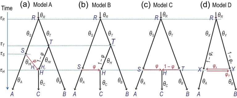
(a)–(d) MSci models A, B, C and D implemented in BPP [81], showing the parameters. In model A, two parental species SH and TH merge to form a hybrid species H at time τ_H, but both parental species become extinct (see Fig. 8(a) and (b) for alternative interpretations). In model B, there is introgression from species RA to TC at time τ_S = τ_H. In model C, species RA and RB come into contact to form hybrid species HC at time τ_S = τ_H = τ_T. Model D assumes bidirectional introgression between species RA and RB at time τ_X = τ_Y. Here the introgression probability (ϕ) is assigned to the horizontal (introgression) branch at each hybridization node, whereas in [81] it is sometimes assigned to the vertical branch.

Four types of MSci model are implemented in bpp (Fig. 7) [81]. In model A, two species SH and TH merge to form a hybrid species HC. This scenario may be rare, but the model can be used to accommodate introgressions involving ghost or unsampled species (Fig. 8(a) and (b)). Model B assumes introgression from species RA to TC at time τ_S = τ_H. This is distinguishable using genetic data from the alternative model in which there is introgression from RB to SC (B₂ in Fig. 8(d)). Model C (Fig. 7(c)) is a case of hybrid speciation. Model D assumes that two species RA and RB came into contact at time τ_X = τ_Y and exchanged migrants.

Figure 8.

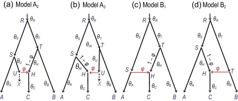
(a) and (b) Two interpretations of model A, alternative to Fig. 7(a), involving a ghost species X. In model A₂, species SUX contributes migrants to species THC at time τ_H and has since become extinct or unsampled in the data, while in model A₃, TUX is the ghost species. Models A₁ (Fig. 7(a)), A₂ and A₃ are indistinguishable using genetic data. (c) and (d) Two versions of model B, which are identifiable using genetic data.

The two parental branches are sometimes called the ‘major hybrid edges’ and ‘minor hybrid edges’, according as , and the binary species tree that remains after all minor hybrid branches are removed is called the ‘major species tree’ [95]. This characterization is useful if gene flow occurs in pulses as assumed by the MSci model, but may be misleading if gene flow is continuous. For example, continuous migration at a low rate per generation can drastically change the gene tree distribution so that, when the MSci model is fitted to the data, the major species tree may reflect gene flow, rather than species divergences [20,72,78].

Below we consider the probabilities of gene tree topologies under the MSci model. These can be used in the two-step methods to estimate the introgression probabilities or to infer the introgression model using reconstructed gene trees as input data, as in the PhyloNet/ML program [96].

The calculation is very similar to that under the simple MSC model (equation (4)). Consider model B (Fig. 9(a)), with three sequences at the locus (a, b, c) [78]. If sequences b and c coalesce in species T, the gene tree will be G₁ = (a, (b, c)), while if a and c coalesce in species S, the gene tree will be G₂ = (b, (c, a)). If neither event occurs, the two coalescent events for the three sequences will occur in species R and the three gene trees will occur with equal probabilities. Thus, G₃ = (c, (a, b)) must be the least probable gene tree. We have

(13)

Figure 9.

(a) MSci model B for three species (Fig. 7(b)) and (b) a gene tree for four sequences for illustrating the gene tree density under the MSci model.

where and are the probabilities that two sequences entering species S or T do not coalesce in that species (cf. φ of equation (3)). Consider gene tree G₁, which means that sequences b and c coalesce first. If sequence c enters S (which happens with probability ϕ), G₁ can occur only if sequences c and a do not coalesce in S. Hence the first term, . If sequence c enters H (which happens with probability 1 − ϕ), sequences b and c can coalesce in T or R. Hence the second term, .

The gene tree probabilities (equations (13)) are functions of ϕ, φ_S and φ_T, while φ_S and φ_T are simple functions of the internal branch lengths in coalescent units on the species tree. We have if (1 − ϕ)(1 − φ_T) < ϕ(1 − φ_S), or if b and c are more likely to coalesce in T than are a and c to coalesce in S [78].

Next we consider the joint density of , the gene tree with the complete history of coalescence and introgression events at locus j, including the parental path taken by each sequence at each hybridization node. This is used in full-likelihood implementations of the MSci model. This joint density is very similar to that under the MSC without gene flow (equation (7)), with the only modification that each time a sequence passes a hybridization node, there is a probability ϕ or 1 − ϕ depending on the parental path taken. Thus, for the gene tree of Fig. 9(b),

(14)

The five pairs of brackets correspond to species C, S, H, T and R (Fig. 9(b)). For species S (i.e. SR), sequence c₁ picks parental path S and coalesces with sequence a at time t₂, so that the contribution to the gene tree density from S is . Introgression is counted as an event in the receiving population (rather than the source population) when we trace the lineages backwards in time and reach a hybridization node.

Bayesian implementations of the introgression model can then proceed as before, with the joint posterior of the MSci model and parameters given by equation (9), except that S now represents the MSci model, the parameter vector Θ includes the introgression probabilities (ϕs) as well as the divergence/introgression times (τs) and population sizes (θs), and the gene tree G_j includes the introgression history at the locus. There are currently three Bayesian MCMC implementations of the MSci model: PhyloNet/MCMC-seq [93], *beast [94,97] and bpp [81] (Table 1). PhyloNet and *beast can allow changes to hybridization events in the MCMC and can infer the introgression model from the data. Those programs appear to reach their limits with <100 loci. Bpp assumes that the MSci model is specified and fixed and the program estimates the parameters under the model. It has been applied to datasets of over 10 000 loci [29,81]. Also, bpp implements four different types of introgression model (Fig. 7), while only model A is available in phyloNet and *beast.

Table 1.

A partial list of computer programs implementing the MSC model with and without gene flow.

Method	MSC	IM & MSci
Full likelihood	3s	3s
	bpp	IMa3
	*beast	G-PhoCS
		bpp
		*beast
		PhyloNet
Two step	astral	PhyloNet
	mp-est	PhyloNetworks
	NJ-st

Binary species trees generated by taking different parental paths at hybridization nodes are called ‘displayed species trees’ [92] or ‘parental species trees’. An interesting formulation of the MSci model specifies the distribution of the gene trees as a mixture over the displayed species trees, with the mixing probabilities given by the introgression probabilities at the hybridization nodes (Fig. 10); see, e.g. [98,99]. To simulate a gene tree, one would sample a displayed species tree first and then generate the gene tree according to the simple MSC model. This is in general incorrect as it forces all sequences at the locus to take the same parental path at each hybridization node, whereas correctly there should be a binomial sampling process when two or more sequences reach a hybridization node. In the model of Fig. 10, if sequences b and c reach species Y, it should be possible for one of them to take the left parent and the other the right parent. In the special case where each hybridization node on the species tree has at most one sequence from all its descendant populations, the formulation is correct and can be used to derive the probability distribution of gene trees. For example, equations (13) for the case of three species and three sequences (Fig. 9(a)) can be derived this way. It is also interesting to note that, under the MSci model, the most probable gene tree may have a topology that is different from all of the displayed species trees [100].

Figure 10.

Displayed species trees are binary trees that result from removing one of the two parental branches at each hybridization node in the MSci model. With k hybridization nodes, there are 2^k displayed species trees. Their probabilities are given by the introgression probabilities at the hybridization nodes: αβ, α(1 − β), (1 − α)β and (1 − α)(1 − β).

Heuristic methods for inferring gene flow

A number of heuristic methods have been developed to test for the presence of gene flow and to estimate its strength. Here we mention a few briefly. The most popular method is the D-statistic or ABBA-BABA test [101]. This uses the species tree (((A, B), C), O) for three species A, B and C, with the outgroup species O, and is based on the counts of site patterns when one sequence or genome is available from each species [102]. There are three parsimony-informative site patterns: AABB matches the species tree, while ABBA and BABA are the mismatching patterns, where A and B are any two distinct nucleotides. The probabilities for the two mismatching site patterns ABBA and BABA should be equal if there exists deep coalescence but no gene flow, but they are different if there is gene flow between the non-sister species (A and C or B and C) in addition to deep coalescence. Thus, gene flow can be tested by using the site-pattern frequencies to examine the deviation of

(15)

from 0. The D-statistic has been extended to the case of five species, assuming a symmetric species tree in the so-called D_FOIL test [103]. The site pattern frequencies can also be used to estimate the introgression probability, as in the program HyDe [104,105]. From

(16)

one gets the estimate

(17)

This is based on the hybridization model with τ_S = τ_T and θ_S = θ_T (Fig. 7(c)). The estimate should be biased if this symmetry does not hold.

A similar argument may be applied to gene tree topologies instead of site patterns(equation 13, Fig. 9(a)). The probabilities of the two mismatching gene trees ((b, c), a) and ((c, a), b) are equal if there exists deep coalescence but no gene flow, but different if there is in addition gene flow between the non-sister species (A and C or B and C). Thus, the observed frequencies of gene tree topologies can be used to estimate the introgression probability, as in the SNaQ method [95,106]. Assume that φ_S = φ_T = φ in equations (13), and let and be the probabilities of the two mismatching gene trees. Then

(18)

The D-statistic cannot be used to detect gene flow between sister species or to estimate the time of introgression. Such unidentifiability issues also exist in other methods that detect hybridization events using genome-wide averages, such as the average interspecies sequence divergence [107] or the joint allele frequency spectrum [108].

Unidentifiability, low information content and challenges of identifying the mode of gene flow

One area where more research is urgently needed is the identifiability of introgression models. If the probability distributions of the data are identical for two sets of parameter values (Θ and Θ^′), with f(X|Θ) = f(X|Θ^′) for essentially every dataset X, then Θ is unidentifiable given data X. Several studies have examined identifiability issues of summary methods that use gene tree topologies as data [76,80,91,109], but little research has been done on full-likelihood methods.

Some cases of unidentifiability are easy to identify. If it is impossible for two or more sequences to be in one species when we trace the genealogical history of the sample backwards in time, the population size (θ) for that species will be unidentifiable, since it takes two sequences to define a distance. For example, in the MSC model with no gene flow (Fig. 2), the population sizes for the extant species are unidentifiable if only one sequence is sampled from each species per locus, but this unidentifiability disappears when multiple sequences are available from each species. Furthermore, parameters or models that are unidentifiable using gene tree topologies alone may become identifiable when both gene trees and branch lengths (coalescent times) are used. In the case of three species, there are only three gene trees, so that use of gene tree topologies can identify only one (under the MSC model) or two (under the MSci model) parameters, whereas there are 7 (Fig. 2) and 13 (Fig. 7(a)) parameters in those two models, respectively, which are all identifiable when information from both gene trees and coalescent times is used.

The identifiability of full-likelihood methods applied to data of multilocus sequence alignments, with multiple sequences per species, is the most interesting case, because full-likelihood methods are expected to be optimal from a statistical point of view and because multilocus alignments are the dominating data form in such analyses. Flouri et al. [81] conjectured that the MSci model is identifiable on multilocus sequence alignments as long as it is identifiable on data of gene trees with coalescent times. Given this, the problem of identifiability can be studied by considering the gene trees with coalescent times (G_j and ) as the input data.

It is noted that MSci model D (Fig. 7(d)) has an unidentifiability issue of the label-switching type [81] (Fig. 11). For every set of parameters, Θ = (θ_R, θ_A, θ_B, θ_X, θ_Y, τ_R, τ_X, ϕ_X, ϕ_Y), there is a ‘mirror’ point Θ^′, which has identical parameter values as Θ except that , , and . Both Θ and Θ^′ have exactly the same likelihood, f(X|S, Θ) = f(X|S, Θ^′), for all possible data X. This is a label-switching issue, and does not affect the utility of the model: one may apply a constraint such as to remove the unidentifiability or apply more sophisticated post-processing of the MCMC sample if the ‘twin towers’ are not well separated [110]. The cases where the bidirectional introgression involves non-sister species or where there are multiple introgression events are yet to be studied.

Figure 11.

MSci model D (bidirectional introgression) (Fig. 7(d)) has an identifiability issue. (a) Model D showing the definitions of parameters. (b) and (c) Two sets of parameter values Θ and Θ^′ that are unidentifiable. The dotted lines indicate the main routes taken by sequences sampled from species A and B, if the introgression probabilities α and β are .

Even if all parameters are identifiable, typical datasets may lack information for their reliable estimation. For example, typical datasets may be highly informative about species divergence times, but not about population sizes for ancestral species, especially if those species correspond to very short branches on the species tree [111]. In the case of three species both gene flow between non-sister species and population structure in the ancestral species can cause the asymmetry in the probabilities of the two mismatching gene trees [112], so that the two models are unidentifiable using gene tree topologies alone. In general, it may be hard to distinguish the different models of gene flow, such as the complete isolation model (MSC with no gene flow), the migration (IM) model, the isolation-with-initial-migration (IIM) model [113] and the introgression (MSci) model. Simulation may be useful to evaluate the power to distinguish such models using genomic datasets.

CONCLUSION

The multispecies coalescent model provides a powerful framework for analysis of genomic sequences sampled from multiple species to extract the rich information about the evolutionary history of the species. Incorporating species phylogeny in population genetic models of population subdivision opens up opportunities for addressing many exciting questions in evolutionary biology, such as detecting gene flow during and after species formation and delineating species boundaries, as well as inferring demographic changes and estimating population sizes for extinct ancestral species. As discussed in [92], the basic MSC model accommodating species phylogeny and coalescent is in effect a null model, which can be extended to include other important biological processes, leading to models such as

• H ₀: MSC (null model),

• H ₁: MSC + migration (MSC+M or IM model),

• H ₂: MSC + introgression (MSC+I or MSci model),

• H ₃: MSC + population structure,

• H ₄: MSC + recombination,

• etc.

Currently, large differences exist between full-likelihood methods and heuristic methods. The former have higher statistical efficiency while the latter are orders-of-magnitude faster computationally. There is thus much room for improvement for both classes of methods. For the present, a pragmatic approach to analyzing large datasets may be to use summary methods to estimate the species tree and then full-likelihood methods to estimate the parameters.

Analysis of the simple three-species case [62] suggests that there is rich historical information both in gene tree branch lengths (which two-step methods such as astral, mp-est and SNaQ ignore) and in the stochastic fluctuation of genealogical history across loci (which genome-averaging approaches such as SVDQuartets and D-statistic ignore). Heuristic methods that make use of both kinds of information may thus have much improved power. For Bayesian implementations of the MSC model, mixing inefficiency of the MCMC algorithm appears to be a far more serious problem than the increase in computational cost for each MCMC iteration [48]. Developing smart proposal algorithms that respect and accommodate the mutual constraints between the species tree and the gene trees is likely to bring dramatic improvement to the capacity of the full-likelihood methods. To empirical biologists, the MSC framework makes it possible to ask exciting evolutionary questions; to method developers, it offers rich opportunities for testing cutting-edge algorithms in computational statistics (in particular, trans-model MCMC algorithms). With the advancements of sequencing technologies and rapid accumulation of genomic sequence data as the driving force, the field will in all likelihood continue to be a research hotspot in the coming years.

REFERENCES

- 1. Kingman JFC. The coalescent. Stoch Process Appl 1982; 13: 235–48. 10.1016/0304-4149(82)90011-4 [DOI] [Google Scholar]
- 2. Hudson RR. Testing the constant-rate neutral allele model with protein sequence data. Evolution 1983; 37: 203–17. 10.1111/j.1558-5646.1983.tb05528.x [DOI] [PubMed] [Google Scholar]
- 3. Tajima F. Evolutionary relationship of DNA sequences in finite populations. Genetics 1983; 105: 437–60. 10.1093/genetics/105.2.437 [DOI] [PMC free article] [PubMed] [Google Scholar]
- 4. Hudson RR. Gene genealogies and the coalescent process. In: Futuyma DJ, Antonovics JD (eds.). Oxford Surveys in Evolutionary Biology. New York: Oxford University Press, 1990, 1–44. [Google Scholar]
- 5. Hein J, Schieriup MH, Wiuf C. Gene Genealogies, Variation and Evolution: a Primer in Coalescent Theory. Oxford: Oxford University Press, 2005. [Google Scholar]
- 6. Nordborg M. Coalescent theory. In: Balding D, Bishop M, Cannings C (eds). Handbook of Statistical Genetics. Chichester, UK: John Wiley, 2007, 843–77. [Google Scholar]
- 7. Wakeley J. Coalescent Theory: An Introduction. Greenwood Village: Roberts & Company, 2009. [Google Scholar]
- 8. Rannala B, Yang Z. Bayes estimation of species divergence times and ancestral population sizes using DNA sequences from multiple loci. Genetics 2003; 164: 1645–56. 10.1093/genetics/164.4.1645 [DOI] [PMC free article] [PubMed] [Google Scholar]
- 9. Xu B, Yang Z. Challenges in species tree estimation under the multispecies coalescent model. Genetics 2016; 204: 1353–68. 10.1534/genetics.116.190173 [DOI] [PMC free article] [PubMed] [Google Scholar]
- 10. Kubatko L. The multispecies coalescent. In: Balding D, Moltke I, Marioni J (eds). Handbook of Statistical Genomics, 4th edn. New York: John Wiley, 2019, 219–45. 10.1002/9781119487845.ch7 [DOI] [Google Scholar]
- 11. Rannala B, Edwards S, Leaché AD, et al. The multispecies coalescent model and species tree inference. In: Scornavacca C, Delsuc F, Galtier N (eds). Phylogenetics in Genomic Era. Section 3.3. No commercial publisher, 2020, 1–21. [Google Scholar]
- 12. Rannala B, Yang Z. Species delimitation. In: Scornavacca C, Delsuc F, Galtier N (eds). Phylogenetics in Genomic Era, Section 5.5. No commercial publisher, 2020, 1–18. [Google Scholar]
- 13. Edwards SV. Is a new and general theory of molecular systematics emerging? Evolution 2009; 63: 1–19. 10.1111/j.1558-5646.2008.00549.x [DOI] [PubMed] [Google Scholar]
- 14. Gillespie JH, Langley CH. Are evolutionary rates really variable. J Mol Evol 1979; 13: 27–34. 10.1007/BF01732751 [DOI] [PubMed] [Google Scholar]
- 15. Takahata N. An attempt to estimate the effective size of the ancestral species common to two extant species from which homologous genes are sequenced. Genet Res 1986; 48: 187–90. 10.1017/S001667230002499X [DOI] [PubMed] [Google Scholar]
- 16. Burgess R, Yang Z. Estimation of hominoid ancestral population sizes under Bayesian coalescent models incorporating mutation rate variation and sequencing errors. Mol Biol Evol 2008; 25: 1979–94. 10.1093/molbev/msn148 [DOI] [PubMed] [Google Scholar]
- 17. Hey J, Nielsen R. Multilocus methods for estimating population sizes, migration rates and divergence time, with applications to the divergence of Drosophila pseudoobscura and D. persimilis. Genetics 2004; 167: 747–60. 10.1534/genetics.103.024182 [DOI] [PMC free article] [PubMed] [Google Scholar]
- 18. Zhu T, Yang Z. Maximum likelihood implementation of an isolation-with-migration model with three species for testing speciation with gene flow. Mol Biol Evol 2012; 29: 3131–42. 10.1093/molbev/mss118 [DOI] [PubMed] [Google Scholar]
- 19. Shi CM, Yang Z. Coalescent-based analyses of genomic sequence data provide a robust resolution of phylogenetic relationships among major groups of gibbons. Mol Biol Evol 2018; 35: 159–79. 10.1093/molbev/msx277 [DOI] [PMC free article] [PubMed] [Google Scholar]
- 20. Thawornwattana Y, Dalquen DA, Yang Z. Coalescent analysis of phylogenomic data confidently resolves the species relationships in the Anopheles gambiae species complex. Mol Biol Evol 2018; 35: 2512–27. 10.1093/molbev/msy158 [DOI] [PMC free article] [PubMed] [Google Scholar]
- 21. Degnan JH, Rosenberg NA. Gene tree discordance, phylogenetic inference and the multispecies coalescent. Trends Ecol Evol 2009; 24: 332–40. 10.1016/j.tree.2009.01.009 [DOI] [PubMed] [Google Scholar]
- 22. Yang Z. Molecular Evolution: A Statistical Approach. Oxford: Oxford University Press, 2014. 10.1093/acprof:oso/9780199602605.001.0001 [DOI] [Google Scholar]
- 23. Liu L, Xi Z, Wu S, et al. Estimating phylogenetic trees from genome-scale data. Ann NY Acad Sci 2015, 1360: 36–53. 10.1111/nyas.12747 [DOI] [PubMed] [Google Scholar]
- 24. Sankararaman S. Methods for detecting introgressed archaic sequences. Curr Opin Genet Dev 2020; 62: 85–90. 10.1016/j.gde.2020.05.026 [DOI] [PMC free article] [PubMed] [Google Scholar]
- 25. Korunes KL, Goldberg A. Human genetic admixture. PLoS Genet 2021; 17: e1009374. 10.1371/journal.pgen.1009374 [DOI] [PMC free article] [PubMed] [Google Scholar]
- 26. Fisher R. The distribution of gene ratios for rare mutations. Proc R Soc Edin 1930; 50: 205–20. [Google Scholar]
- 27. Wright S. Evolution in Mendelian populations. Genetics 1931; 16: 97–159. 10.1093/genetics/16.2.97 [DOI] [PMC free article] [PubMed] [Google Scholar]
- 28. Yu N, Chen FC, Ota S, et al. Larger genetic differences within Africans than between Africans and Eurasians. Genetics 2002; 161: 269–74. 10.1093/genetics/161.1.269 [DOI] [PMC free article] [PubMed] [Google Scholar]
- 29. Thawornwattana Y, Mallet J, Yang Z. Complex introgression history of the erato-sara clade of Heliconius butterflies, bioRxiv, 2021; doi: 10.1101/2021.02.10.430600. [Google Scholar]
- 30. Edwards AWF. Estimation of the branch points of a branching diffusion process. J R Stat Soc B 1970; 32: 155–64. [Google Scholar]
- 31. Takahata N. Gene genealogy in three related populations: consistency probability between gene and population trees. Genetics 1989; 122: 957–66. 10.1093/genetics/122.4.957 [DOI] [PMC free article] [PubMed] [Google Scholar]
- 32. Liu L, Edwards SV. Phylogenetic analysis in the anomaly zone. Syst Biol 2009; 58: 452–60. 10.1093/sysbio/syp034 [DOI] [PubMed] [Google Scholar]
- 33. Degnan JH, Salter LA. Gene tree distributions under the coalescent process. Evolution 2005; 59: 24–37. 10.1111/j.0014-3820.2005.tb00891.x [DOI] [PubMed] [Google Scholar]
- 34. Degnan JH, Rosenberg NA. Discordance of species trees with their most likely gene trees. PLoS Genet 2006; 2: e68. 10.1371/journal.pgen.0020068 [DOI] [PMC free article] [PubMed] [Google Scholar]
- 35. Pamilo P, Nei M. Relationships between gene trees and species trees. Mol Biol Evol 1988; 5: 568–83. [DOI] [PubMed] [Google Scholar]
- 36. Linkem CW, Minin VN, Leaché AD . Detecting the anomaly zone in species trees and evidence for a misleading signal in higher-level skink phylogeny (Squamata: Scincidae). Syst Biol 2016; 65: 465–77. 10.1093/sysbio/syw001 [DOI] [PMC free article] [PubMed] [Google Scholar]
- 37. Cloutier A, Sackton TB, Grayson P, et al. Whole-genome analyses resolve the phylogeny of flightless birds (Palaeognathae) in the presence of an empirical anomaly zone. Syst Biol 2019; 68: 937–55. 10.1093/sysbio/syz019 [DOI] [PMC free article] [PubMed] [Google Scholar]
- 38. Wu Y. Coalescent-based species tree inference from gene tree topologies under incomplete lineage sorting by maximum likelihood. Evolution 2012; 66: 763–75. 10.1111/j.1558-5646.2011.01476.x [DOI] [PubMed] [Google Scholar]
- 39. Liu L, Yu L, Edwards SV. A maximum pseudo-likelihood approach for estimating species trees under the coalescent model. BMC Evol Biol 2010; 10: 302. 10.1186/1471-2148-10-302 [DOI] [PMC free article] [PubMed] [Google Scholar]
- 40. Mirarab S, Warnow T. ASTRAL-II: coalescent-based species tree estimation with many hundreds of taxa and thousands of genes. Bioinformatics 2015; 31: i44–52. 10.1093/bioinformatics/btv234 [DOI] [PMC free article] [PubMed] [Google Scholar]
- 41. Maddison WP. Gene trees in species trees. Syst Biol 1997; 46: 523–36. 10.1093/sysbio/46.3.523 [DOI] [Google Scholar]
- 42. Nichols R. Gene trees and species trees are not the same. Trends Ecol Evol 2001; 16: 358–64. 10.1016/S0169-5347(01)02203-0 [DOI] [PubMed] [Google Scholar]
- 43. Edwards SV, Jennings WB, Shedlock AM. Phylogenetics of modern birds in the era of genomics. Proc R Soc B 2005; 272: 979–92. 10.1098/rspb.2004.3035 [DOI] [PMC free article] [PubMed] [Google Scholar]
- 44. Yang Z. Likelihood and Bayes estimation of ancestral population sizes in hominoids using data from multiple loci. Genetics 2002; 162: 1811–23. 10.1093/genetics/162.4.1811 [DOI] [PMC free article] [PubMed] [Google Scholar]
- 45. Dalquen D, Zhu T, Yang Z. Maximum likelihood implementation of an isolation-with-migration model for three species. Syst Biol 2017; 66: 379–98. [DOI] [PubMed] [Google Scholar]
- 46. Heled J, Drummond AJ. Bayesian inference of species trees from multilocus data. Mol Biol Evol 2010; 27: 570–80. 10.1093/molbev/msp274 [DOI] [PMC free article] [PubMed] [Google Scholar]
- 47. Yang Z, Rannala B. Unguided species delimitation using DNA sequence data from multiple loci. Mol Biol Evol 2014; 31: 3125–35. 10.1093/molbev/msu279 [DOI] [PMC free article] [PubMed] [Google Scholar]
- 48. Rannala B, Yang Z. Efficient Bayesian species tree inference under the multispecies coalescent. Syst Biol 2017; 66: 823–42. 10.1093/sysbio/syw119 [DOI] [PMC free article] [PubMed] [Google Scholar]
- 49. Flouri T, Jiao X, Rannala B, et al. Species tree inference with BPP using genomic sequences and the multispecies coalescent. Mol Biol Evol 2018; 35: 2585–93. 10.1093/molbev/msy147 [DOI] [PMC free article] [PubMed] [Google Scholar]
- 50. Felsenstein J. Evolutionary trees from DNA sequences: a maximum likelihood approach. J Mol Evol 1981; 17: 368–76. 10.1007/BF01734359 [DOI] [PubMed] [Google Scholar]
- 51. Hey J, Nielsen R. Integration within the Felsenstein equation for improved Markov chain Monte Carlo methods in population genetics. Proc Natl Acad Sci USA 2007; 104: 2785–90. 10.1073/pnas.0611164104 [DOI] [PMC free article] [PubMed] [Google Scholar]
- 52. Yang Z, Rannala B. Bayesian species delimitation using multilocus sequence data. Proc Natl Acad Sci USA 2010; 107: 9264–9. 10.1073/pnas.0913022107 [DOI] [PMC free article] [PubMed] [Google Scholar]
- 53. Liu L, Pearl DK. Species trees from gene trees: reconstructing Bayesian posterior distributions of a species phylogeny using estimated gene tree distributions. Syst Biol 2007; 56: 504–14. 10.1080/10635150701429982 [DOI] [PubMed] [Google Scholar]
- 54. Ronquist F, Huelsenbeck JP. MrBayes 3: Bayesian phylogenetic inference under mixed models. Bioinformatics 2003; 19: 1572–4. 10.1093/bioinformatics/btg180 [DOI] [PubMed] [Google Scholar]
- 55. Jones G. Algorithmic improvements to species delimitation and phylogeny estimation under the multispecies coalescent. J Math Biol 2017; 74: 447–67. 10.1007/s00285-016-1034-0 [DOI] [PubMed] [Google Scholar]
- 56. Ogilvie HA, Bouckaert RR, Drummond AJ. StarBEAST2 brings faster species tree inference and accurate estimates of substitution rates. Mol Biol Evol 2017; 34: 2101–14. 10.1093/molbev/msx126 [DOI] [PMC free article] [PubMed] [Google Scholar]
- 57. Liu L, Yu L. Estimating species trees from unrooted gene trees. Syst Biol 2011; 60: 661–7. 10.1093/sysbio/syr027 [DOI] [PubMed] [Google Scholar]
- 58. Chifman J, Kubatko LS. Quartet inference from SNP data under the coalescent model. Bioinformatics 2014; 30: 3317–24. 10.1093/bioinformatics/btu530 [DOI] [PMC free article] [PubMed] [Google Scholar]
- 59. Sayyari E, Mirarab S. Fast coalescent-based computation of local branch support from quartet frequencies. Mol Biol Evol 2016; 33: 1654–68. 10.1093/molbev/msw079 [DOI] [PMC free article] [PubMed] [Google Scholar]
- 60. Huang H, Knowles LL. What is the danger of the anomaly zone for empirical phylogenetics? Syst Biol 2009; 58: 527–36. 10.1093/sysbio/syp047 [DOI] [PubMed] [Google Scholar]
- 61. Andersen LN, Mailund T, Hobolth A. Efficient computation in the IM model. J Math Biol 2014; 68: 1423–51. 10.1007/s00285-013-0671-9 [DOI] [PubMed] [Google Scholar]
- 62. Zhu T, Yang Z. Complexity of the simplest species tree problem. Mol Biol Evol 2021; doi: 10.1093/molbev/msab009. [DOI] [PMC free article] [PubMed] [Google Scholar]
- 63. Liu L, Yu L, Pearl DK. Maximum tree: a consistent estimator of the species tree. J Math Biol 2010; 60: 95–106. 10.1007/s00285-009-0260-0 [DOI] [PubMed] [Google Scholar]
- 64. Leaché AD, Rannala B. The accuracy of species tree estimation under simulation: a comparison of methods. Syst Biol 2010; 60: 126–37. [DOI] [PubMed] [Google Scholar]
- 65. DeGiorgio M, Degnan JH. Robustness to divergence time underestimation when inferring species trees from estimated gene trees. Syst Biol 2014; 63: 66–82. 10.1093/sysbio/syt059 [DOI] [PubMed] [Google Scholar]
- 66. Jukes TH, Cantor CR. Evolution of Protein Molecules. In: Munro HN (ed.). Mammalian Protein Metabolism. New York: Academic Press, 1969, 21–123. 10.1016/B978-1-4832-3211-9.50009-7 [DOI] [Google Scholar]
- 67. Roch S, Steel M. Likelihood-based tree reconstruction on a concatenation of aligned sequence data sets can be statistically inconsistent. Theor Popul Biol 2015; 100: 56–62. 10.1016/j.tpb.2014.12.005 [DOI] [PubMed] [Google Scholar]
- 68. Kim A, Degnan JH. PRANC: ML species tree estimation from the ranked gene trees under coalescence. Bioinformatics 2020; 36: 4819–21. 10.1093/bioinformatics/btaa605 [DOI] [PMC free article] [PubMed] [Google Scholar]
- 69. Baack EJ, Rieseberg LH. A genomic view of introgression and hybrid speciation. Curr Opin Genet Dev 2007; 17: 513–8. 10.1016/j.gde.2007.09.001 [DOI] [PMC free article] [PubMed] [Google Scholar]
- 70. Mallet J, Besansky N, Hahn MW. How reticulated are species? BioEssays 2016; 38: 140–9. 10.1002/bies.201500149 [DOI] [PMC free article] [PubMed] [Google Scholar]
- 71. Martin SH, Jiggins CD. Interpreting the genomic landscape of introgression. Curr Opin Genet Dev 2017; 47: 69–74. 10.1016/j.gde.2017.08.007 [DOI] [PubMed] [Google Scholar]
- 72. Fontaine MC, Pease JB, Steele A, et al. Extensive introgression in a malaria vector species complex revealed by phylogenomics. Science 2015; 347: 1258524. 10.1126/science.1258524 [DOI] [PMC free article] [PubMed] [Google Scholar]
- 73. Martin SH, Dasmahapatra KK, Nadeau NJ, et al. Genome-wide evidence for speciation with gene flow in Heliconius butterflies. Genome Res 2013; 23: 1817–28. 10.1101/gr.159426.113 [DOI] [PMC free article] [PubMed] [Google Scholar]
- 74. Nielsen R, Akey JM, Jakobsson M, et al. Tracing the peopling of the world through genomics. Nature 2017; 541: 302–10. 10.1038/nature21347 [DOI] [PMC free article] [PubMed] [Google Scholar]
- 75. Leaché AD, Harris RB, Rannala B, et al. The influence of gene flow on Bayesian species tree estimation: a simulation study. Syst Biol 2014; 63: 17–30. 10.1093/sysbio/syt049 [DOI] [PubMed] [Google Scholar]
- 76. Solis-Lemus C, Yang M, Ane C. Inconsistency of species tree methods under gene flow. Syst Biol 2016; 65: 843–51. 10.1093/sysbio/syw030 [DOI] [PubMed] [Google Scholar]
- 77. Long C, Kubatko LS. The effect of gene flow on coalescent-based species-tree inference. Syst Biol 2018; 67: 770–85. 10.1093/sysbio/syy020 [DOI] [PubMed] [Google Scholar]
- 78. Jiao X, Flouri T, Rannala B, et al. The impact of cross-species gene flow on species tree estimation. Syst Biol 2020; 69: 830–47. 10.1093/sysbio/syaa001 [DOI] [PubMed] [Google Scholar]
- 79. Nielsen R, Wakeley J. Distinguishing migration from isolation: a Markov chain Monte Carlo approach. Genetics 2001; 158: 885–96. 10.1093/genetics/158.2.885 [DOI] [PMC free article] [PubMed] [Google Scholar]
- 80. Yu Y, Degnan JH, Nakhleh L. The probability of a gene tree topology within a phylogenetic network with applications to hybridization detection. PLoS Genet 2012; 8: e1002660. 10.1371/journal.pgen.1002660 [DOI] [PMC free article] [PubMed] [Google Scholar]
- 81. Flouri T, Jiao X, Rannala B, et al. A Bayesian implementation of the multispecies coalescent model with introgression for phylogenomic analysis. Mol Biol Evol 2020; 37: 1211–23. 10.1093/molbev/msz296 [DOI] [PMC free article] [PubMed] [Google Scholar]
- 82. Notohara M. The coalescent and the genealogical process in geographically structured populations. J Math Biol 1990; 29: 59–75. 10.1007/BF00173909 [DOI] [PubMed] [Google Scholar]
- 83. Nath HB, Griffiths RC. The coalescent in two colonies with symmetric migration. J Math Biol 1993; 31: 841–52. 10.1007/BF00168049 [DOI] [PubMed] [Google Scholar]
- 84. Wilkinson-Herbots HM. Genealogy and subpopulation differentiation under various models of population structure. J Math Biol 1998; 37: 535–85. 10.1007/s002850050140 [DOI] [Google Scholar]
- 85. Beerli P, Felsenstein J. Maximum-likelihood estimation of migration rates and effective population numbers in two populations using a coalescent approach. Genetics 1999; 152: 763–73. 10.1093/genetics/152.2.763 [DOI] [PMC free article] [PubMed] [Google Scholar]
- 86. Beerli P, Felsenstein J. Maximum likelihood estimation of a migration matrix and effective population sizes in n subpopulations by using a coalescent approach. Proc Natl Acad Sci USA 2001; 98: 4563–8. 10.1073/pnas.081068098 [DOI] [PMC free article] [PubMed] [Google Scholar]
- 87. Wang Y, Hey J. Estimating divergence parameters with small samples from a large number of loci. Genetics 2010; 184: 363–79. 10.1534/genetics.109.110528 [DOI] [PMC free article] [PubMed] [Google Scholar]
- 88. Hey J. Isolation with migration models for more than two populations. Mol Biol Evol 2010; 27: 905–20. 10.1093/molbev/msp296 [DOI] [PMC free article] [PubMed] [Google Scholar]
- 89. Hey J, Chung Y, Sethuraman A, et al. Phylogeny estimation by integration over isolation with migration models. Mol Biol Evol 2018; 35: 2805–18. [DOI] [PMC free article] [PubMed] [Google Scholar]
- 90. Gronau I, Hubisz MJ, Gulko B, et al. Bayesian inference of ancient human demography from individual genome sequences. Nat Genet 2011; 43: 1031–4. 10.1038/ng.937 [DOI] [PMC free article] [PubMed] [Google Scholar]
- 91. Zhu S, Degnan J. Displayed trees do not determine distinguishability under the network multispecies coalescent. Syst Biol 2017; 66: 283–98. [DOI] [PMC free article] [PubMed] [Google Scholar]
- 92. Degnan JH. Modeling hybridization under the network multispecies coalescent. Syst Biol 2018; 67: 786–99. 10.1093/sysbio/syy040 [DOI] [PMC free article] [PubMed] [Google Scholar]
- 93. Wen D, Nakhleh L. Coestimating reticulate phylogenies and gene trees from multilocus sequence data. Syst Biol 2018; 67: 439–57. 10.1093/sysbio/syx085 [DOI] [PubMed] [Google Scholar]
- 94. Zhang C, Ogilvie HA, Drummond AJ, et al. Bayesian inference of species networks from multilocus sequence data. Mol Biol Evol 2018; 35: 504–17. 10.1093/molbev/msx307 [DOI] [PMC free article] [PubMed] [Google Scholar]
- 95. Solis-Lemus C, Bastide P, Ane C. PhyloNetworks: a package for phylogenetic networks. Mol Biol Evol 2017; 34: 3292–8. 10.1093/molbev/msx235 [DOI] [PubMed] [Google Scholar]
- 96. Yu Y, Dong J, Liu KJ, et al. Maximum likelihood inference of reticulate evolutionary histories. Proc Natl Acad Sci USA 2014; 111: 16448–53. 10.1073/pnas.1407950111 [DOI] [PMC free article] [PubMed] [Google Scholar]
- 97. Jones GR. Divergence estimation in the presence of incomplete lineage sorting and migration. Syst Biol 2019; 68: 19–31. [DOI] [PubMed] [Google Scholar]
- 98. Kubatko LS. Identifying hybridization events in the presence of coalescence via model selection. Syst Biol 2009; 58: 478–88. 10.1093/sysbio/syp055 [DOI] [PubMed] [Google Scholar]
- 99. Meng C, Kubatko LS. Detecting hybrid speciation in the presence of incomplete lineage sorting using gene tree incongruence: a model. Theor Popul Biol 2009; 75: 35–45. 10.1016/j.tpb.2008.10.004 [DOI] [PubMed] [Google Scholar]
- 100. Zhu J, Yu Y, Nakhleh L. In the light of deep coalescence: revisiting trees within networks. BMC Bioinform 2016; 17: 415. 10.1186/s12859-016-1269-1 [DOI] [PMC free article] [PubMed] [Google Scholar]
- 101. Durand EY, Patterson N, Reich D, et al. Testing for ancient admixture between closely related populations. Mol Biol Evol 2011; 28: 2239–52. 10.1093/molbev/msr048 [DOI] [PMC free article] [PubMed] [Google Scholar]
- 102. Patterson N, Moorjani P, Luo Y, et al. Ancient admixture in human history. Genetics 2012; 192: 1065–93. 10.1534/genetics.112.145037 [DOI] [PMC free article] [PubMed] [Google Scholar]
- 103. Pease JB, Hahn MW. Detection and polarization of introgression in a five-taxon phylogeny. Syst Biol 2015; 64: 651–62. 10.1093/sysbio/syv023 [DOI] [PubMed] [Google Scholar]
- 104. Blischak PD, Chifman J, Wolfe AD, et al. HyDe: a Python package for genome-scale hybridization detection. Syst Biol 2018; 67: 821–9. 10.1093/sysbio/syy023 [DOI] [PMC free article] [PubMed] [Google Scholar]
- 105. Kubatko LS, Chifman J. An invariants-based method for efficient identification of hybrid species from large-scale genomic data. BMC Evol Biol 2019; 19: 112. 10.1186/s12862-019-1439-7 [DOI] [PMC free article] [PubMed] [Google Scholar]
- 106. Solis-Lemus C, Ane C. Inferring phylogenetic networks with maximum pseudolikelihood under incomplete lineage sorting. PLoS Genet 2016; 12: e1005896. 10.1371/journal.pgen.1005896 [DOI] [PMC free article] [PubMed] [Google Scholar]
- 107. Aeschbacher S, Selby JP, Willis JH, et al. Population-genomic inference of the strength and timing of selection against gene flow. Proc Natl Acad Sci USA 2017; 114: 7061–6. 10.1073/pnas.1616755114 [DOI] [PMC free article] [PubMed] [Google Scholar]
- 108. Kern AD, Hey J. Exact calculation of the joint allele frequency spectrum for isolation with migration models. Genetics 2017; 207: 241–53. 10.1534/genetics.116.194019 [DOI] [PMC free article] [PubMed] [Google Scholar]
- 109. Pardi F, Scornavacca C. Reconstructible phylogenetic networks: do not distinguish the indistinguishable. PLoS Comput Biol 2015; 11: e1004135. 10.1371/journal.pcbi.1004135 [DOI] [PMC free article] [PubMed] [Google Scholar]
- 110. Stephens M. Dealing with label switching in mixture models. J R Statist Soc B 2000; 62: 795–809. 10.1111/1467-9868.00265 [DOI] [Google Scholar]
- 111. Huang J, Flouri T, Yang Z. A simulation study to examine the information content in phylogenomic datasets under the multispecies coalescent model. Mol Biol Evol 2020; 37: 3211–24. 10.1093/molbev/msaa166 [DOI] [PubMed] [Google Scholar]
- 112. Slatkin M, Pollack JL. Subdivision in an ancestral species creates asymmetry in gene trees. Mol Biol Evol 2008; 25: 2241–6. 10.1093/molbev/msn172 [DOI] [PMC free article] [PubMed] [Google Scholar]
- 113. Costa RJ, Wilkinson-Herbots H. Inference of gene flow in the process of speciation: an efficient maximum-likelihood method for the isolation-with-initial-migration model. Genetics 2017; 205: 1597–618. 10.1534/genetics.116.188060 [DOI] [PMC free article] [PubMed] [Google Scholar]
Associated Data
This section collects any data citations, data availability statements, or supplementary materials included in this article.