

Abstract
Motivation
Human proteins that are secreted into different body fluids from various cells and tissues can be promising disease indicators. Modern proteomics research empowered by both qualitative and quantitative profiling techniques has made great progress in protein discovery in various human fluids. However, due to the large number of proteins and diverse modifications present in the fluids, as well as the existing technical limits of major proteomics platforms (e.g. mass spectrometry), large discrepancies are often generated from different experimental studies. As a result, a comprehensive proteomics landscape across major human fluids are not well determined.
Results
To bridge this gap, we have developed a deep learning framework, named DeepSec, to identify secreted proteins in 12 types of human body fluids. DeepSec adopts an end-to-end sequence-based approach, where a Convolutional Neural Network is built to learn the abstract sequence features followed by a Bidirectional Gated Recurrent Unit with fully connected layer for protein classification. DeepSec has demonstrated promising performances with average area under the ROC curves of 0.85–0.94 on testing datasets in each type of fluids, which outperforms existing state-of-the-art methods available mostly on blood proteins. As an illustration of how to apply DeepSec in biomarker discovery research, we conducted a case study on kidney cancer by using genomics data from the cancer genome atlas and have identified 104 possible marker proteins.
Availability
DeepSec is available at https://bmbl.bmi.osumc.edu/deepsec/.
Supplementary information
Supplementary data are available at Bioinformatics online.
1 Introduction
Human body fluids, such as blood, saliva and urine, are primary clinical specimens, which hold considerable promises in presenting molecular biomarkers for disease diagnosis and therapeutic monitoring (Anderson, 2010; Lathrop et al., 2003). Since the first study of serum globulin was reported in 1937 (Tiselius, 1937), several large-scale research efforts have been made to profile proteomes in various types of human body fluids, mostly in blood, using different proteomic technologies, such as two-dimensional gel electrophoresis (Margolis and Kenrick, 1969), mass spectrometry (Thomson, 1914) and liquid chromatography (Zhao and Lin, 2014). As a result, a large number of protein species were identified in different body fluids, which have been documented in a large volume of research papers and archived in several community-based proteomic databases such as Human Plasma Proteome Project (Legrain et al., 2011), Plasma Proteome Database (Nanjappa et al., 2014) and Human Plasma PeptideAtlas (Schwenk et al., 2017).
Due to the large complexity of protein content and post-modifications involved in different body fluids, protein identification using conventional proteomics techniques remains a challenging research topic in the past decade. To facilitate this research, several computational attempts have been made to predict secreted proteins in human body fluids, mostly based on machine learning methods, such as Support Vector Machine (SVM) (Cui et al., 2008; Hong et al., 2011; Sun et al., 2015; Wang et al., 2013, 2016b). These models often used common protein features such as amino acid flexibility index, surface tension and solubility as input and predict secreted proteins associated with a specific body fluid. Although the performances of those methods were promising, featured-based models generally suffered from common limitations such as the blind manual collection of features that might be incomplete and biased and feature selection procedures that need manual intervention. To this end, automatic feature extraction using end-to-end model can dispense with the initial feature selection step and possibly improve the prediction performance.
Deep learning (DL) has been successfully applied in protein research to study new protein functions, structures and interactions (Jain et al., 2021). Among different DL models, Convolutional Neural Network (CNN) has been one of the most frequently used methods and has attained remarkable performances in several classification applications, especially when combined with Gated Recurrent Unit (GRU) (Wilaiprasitporn et al., 2020). GRU, as a new class of Recurrent Neural Networks (RNNs), can effectviely solve the vanishing gradient problem by introducing memory cells and a gating mechanism for holding information from the prior inputs in a well-behaved way. Compared to Long Short-Term Memory, GRU has a relatively simple structure, which ensures reduced complexity and faster convergence. Recent successes with GRU on the basis of protein sequences include DeepSig (a model to detect signal peptides of proteins) (Savojardo et al., 2018) and DeepLoc (a model for predicting protein subcellular localization) (Armenteros et al., 2017). The high performances from both studies indicate that protein sequences must carry important characteristics related to protein sorting.
In this study, we present a new DL-framework, named DeepSec, to facilitate body-fluid secreted protein prediction. DeepSec adopts an end-to-end sequence-based approach and employs CNN as a feature extractor and Bidirectional Gated Recurrent Unit (BGRU) with fully connected dense layer as a classifier to predict secreted proteins. We have employed DeepSec on 12 different types of common human body fluids (one model for each body fluid), which include blood, saliva, urine, cerebrospinal fluid, seminal fluid, amniotic fluid, tear fluid, bronchoalveolar lavage fluid, milk, nipple aspirate fluid, pleural effusion and sputum. At last, we demonstrate possible applications of DeepSec in biomarker discovery by a kidney cancer case study.
2 Materials and methods
2.1 Datasets
The positive datasets of DeepSec were collected from our previous work (Huang et al., 2021). For negative dataset generation, we employed a similar method that is proposed by Cui et al. (2008), where the Pfam family annotation was used to select proteins that are potential non-body-fluid-secretory proteins. We chose negative samples from Pfam families (Pfam release 33.1) (Sara et al., 2018) which do not contain any proteins in the positive dataset. According to the size of the positive dataset varies in different fluid type, the selection of negative samples is carried out as follows. For a specific body fluid, if the count of positive-related Pfam families is greater than 30% of the total number of human-related Pfam families, all proteins in the remaining Pfam families were collected as the negative set. In contrast, if the count is <30%, we randomly chose one member from each remaining Pfam families to construct the negative data.
Using the above procedure, we have collected both positive and negative datasets for each of the 12 body fluids (Fig. 1), including 8203 and 2739 proteins in blood, 4072 and 3291 proteins in saliva, 8048 and 5136 proteins in urine, 6260 and 5787 proteins in cerebrospinal fluid, 5576 and 2624 proteins in seminal fluid, 3212 and 3722 proteins in amniotic fluid, 1490 and 4184 proteins in tear fluid, 1117 and 4436 proteins in bronchoalveolar lavage fluid, 2171 and 3887 proteins in milk, 2234 and 4009 proteins in nipple aspirate fluid, 1373 and 4328 proteins in pleural effusion, and 2341 and 3967 proteins in sputum.
Fig. 1.
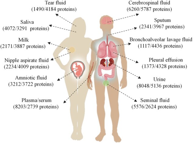
The distribution of 12 types of body fluids that are analyzed in this study
Training DL models generally benefits from datasets with a balanced size. To address the imbalance problem, a random under-sampling process is adopted in this study, which is advantageous over the procedure of eliminating proteins from the over-sized larger dataset to match the size of smaller dataset that may lead to information loss. We randomly partitioned the larger dataset into smaller subsets with similar size of the smaller dataset. For a size ratio between the positive and negative datasets, subsets are created randomly. Each generated new subset and the original smaller dataset are resampled together to generate independent datasets for model evaluation. At last, bagging algorithm is employed to calculate the overall performance of the model, i.e. the average performance across all sample model denoted as where refers to the performance based on one sample set.
Furthermore, the sample space of each body fluid is divided into training, validation and testing datasets according to the proportion of 60%, 20% and 20%, respectively.
2.2 Neural network model
DeepSec takes protein sequences as input and performs a binary classification in terms of secretion into a specific body fluid or not. Figure 2 summarizes the architecture of DeepSec, which comprises three basic components: input sequences, feature extraction and classification.
Fig. 2.

The architecture of DeepSec which supports input as PSI-profiles based on protein sequences, feature extraction through CNN, classification based on BGRU with fully connected dense layer, and the outputs as the probability of being secreted protein
2.2.1 Input sequence generation
We first create a Position-Specific Score Matrix (PSSM) for each protein sequence to enable subsequent convolution operations. The protein sequence is embodied into a PSSM by position-specific iterative basic local alignment search (PSI-BLAST) (Altschul et al., 1997) against UniRef 90 (released in 2020_01) database with inclusion 0.001 and 3 iterations. For each protein with sequence length , a PSSM of dimensionality is obtained. The columns of PSSM represent the presence of 20 amino acids in each position. We then transform the PSSM described in Wang et al. (2016a) by the Sigmoid function where represents a single entry of the PSSM.
Since variable sequence length [from tens to thousands of amino acids (aa) in this case] represents another challenge for building the prediction model, we decide to use a fixed size (1000aa) window to process protein sequences. It has been shown that N-terminus or C-terminus of the sequence carry the most useful signaling information. For instance, N-terminal modifications have a pivotal role in protein regulation and cellular signaling (Varland et al., 2015), and the identity of the C-terminal amino acids has a strong influence on protein expression levels (Weber et al., 2020). Therefore, if a protein’s length exceeds 1000, we will keep 500 aa from N-terminus and C-terminus, respectively, and remove the middle sequence. This method of fixed size window has achieved remarkable performances in protein localization prediction (Armenteros et al., 2017). In the training dataset, 11.7% of the proteins are truncated using this rule. If a protein sequence is <1000aa, the missing part is filled with 0. As a result, the input representation of each protein is a matrix with size [sequence length () size of amino acid vocabulary ()].
2.2.2 Feature extraction
To reveal hidden knowledge from the observed PSSM, a CNN model is trained to extract a complex feature representation of the input sequence. Specifically, the input PSSM matrix is fed into CNN to learn the weight parameters of the convolution filters. The filters are set to calculate the feature map . The convolution layer outputs the matrix inner product between the input matrix and the filters. The rectified linear unit (ReLU) was applied as the activation function to sparsify the output of the convolution layer:
| (1) |
where is the PSSM matrix, is th the weight matrix of the convolution kernels, is the offset vector, is the results of feature extraction. Then, is used as input to feed into the next layer.
2.2.3 Classification
For memorizing the residue presence in the C-terminus and N-terminus, respectively, we use the forwards and backwards GRU to capture possible long-range dependencies between the sequence and the prediction. Bidirectional GRU sweeps from both C-terminus to N-terminus and N-terminus to C-terminus, and concatenates the outputs of individual directions before feeding them into the fully connected layer. The hidden states are updated recursively from the convolutional features and the previous value of the hidden states (Fig. 3).
Fig. 3.
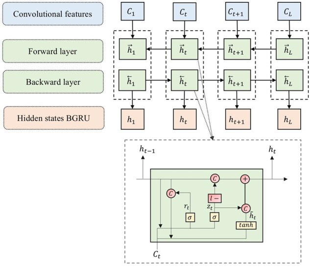
The forwards and backwards GRU capturing possible long-range dependencies between the input sequence and the predicted class
The recurrent calculation at each sequence position is denoted as:
| (2) |
| (3) |
| (4) |
| (5) |
| (6) |
where is the input features of at position , is the hidden states of BGRU, where is a vector of 2-time size of the number of hidden units in the individual direction GRU, ,, , , and are the weight metrics and , and are the bias. The calculation of is similar to . The function is a non-linear activation function taking the form of .
Then, the subsequence classification is performed by a fully connected layer comprised hidden-layers and an output layer. The hidden layer computes a non-linear transformation, defined as follows:
| (7) |
where and are the weight vector and bias respectively, is the learned hidden states of BGRU, ReLU activation is used.
Finally, the output layer computes the probability distribution , defined as follow:
| (8) |
where and are the weight vector and the bias respectively, and the function is the softmax function, denoted as , for .
A cross-entropy loss function is used to quantify how ‘far away’ our prediction is from the ground truth. Network parameters are optimized by minimizing the training errors. The backward pass uses the chain rule to back-propagate error signals and computes gradients with respect to all weights throughout the neural network. Given a training set , is the number of samples and is the true output targets, the cross-entropy loss function is defined as:
| (9) |
2.3 Performance assessment
The prediction performance is measured based on both training and validation sets. Specifically, accuracy, Matthew’s correlation coefficient (MCC) and the Area under the ROC Curve (AUC) are applied. Considering the unbalanced cases in this study, we also include additional measures including precision, recall and F-measure. Note that higher values indicate better classification performance for all those measures.
Accuracy represents how many predictions of the classifier are in fact correct, defined as:
| (10) |
where and are the true predictions in positives and negatives, respectively, and and are the false predictions in positives and negatives, respectively.
Recall (or sensitivity) shows how many positive examples are correctly identified by the classifier. In this case, this is the percentage of secreted proteins identified as such, defined as:
| (11) |
Precision represents the proportion of the correctly predicted positive cases relative to all the predicted positive ones. In this case, this is the percentage of proteins identified as secreted proteins that actually secreted proteins, defined as:
| (12) |
F-measure is the harmonic mean of precision and recall, and better reflects the performance of a classifier of unbalanced classes, defined as:
| (13) |
MCC is a correlation coefficient between the observed and predicted binary classifications, defined as:
| (14) |
2.4 Comparison with other models based on protein features
Since SVM has been previously applied for secreted protein prediction, we first compare DeepSec with SVM models based on reported protein features. In addition, two other state-of-the-art models, including Decision Tree (DT) and Deep Neural Network (DNN), are benchmarked together with DeepSec. To do this, we use the same datasets to evaluate the performance to ensure a fairy comparison. We examine features used in the previous studies and also add a few newly reported features, which can be grouped into four categories: (i) sequence properties; (ii) physicochemical properties; (iii) domains/motifs properties; and (iv) structural properties. In total, a total of 1610 protein features are collected (as detailed in Supplementary Table S1). Then, feature selection is performed in a similar workflow as documented in our previous publication (Huang et al., 2021), where -test () and false discovery rate (FDR, ) are employed to rank the features. The top 50 features are selected into the final model for 12 body fluids, respectively (Supplementary Table S2). Feature normalization is performed using Z-score method. Finally, these models are evaluated in terms of accuracy, recall, precision, F-measure, MCC and AUC.
3 Results
3.1 Model performance of DeepSec in 12 types of body fluid
All classification models on 12 body fluids were built and evaluated using Pytorch 1.7.1, running python 3.8 and using Scikit-learn library version 0.23.2. In DeepSec, the input representation of each protein is a matrix. Referring to Deeploc (Armenteros et al., 2017), our model has 50 filters at the convolution layer with three different sizes =, which has led to a total of 150 filters and feature maps. Next, GRU scanned the sequence using 32 hidden units in each individual direction, leading to a total of outputs. The fully connected layer comprised a single hidden-layer with 16 units and an output layer with two units. The parameters were optimized by Adam optimizer with learning rate as 0.0001 and a dropout probability as 0.1 prior to fully connected layer. We chose 0.5 as the prediction threshold, which means that a probability indicates a positive class associated with secretion into a specific body fluid. Finally, the performances on 12 body fluids were evaluated based on testing dataset (Table 1) and all datasets (Table 2), respectively.
Table 1.
The performance evaluation on 12 body fluids based on testing dataset, grouped by several evaluation measures
| Body fluids | Accuracy | Recall | Precision | F-measure | MCC | AUC |
|---|---|---|---|---|---|---|
| Blood | 0.871139 | 0.872120 | 0.868200 | 0.910294 | 0.691481 | 0.940572 |
| Saliva | 0.824650 | 0.810522 | 0.835108 | 0.797251 | 0.643117 | 0.898319 |
| Urine | 0.845857 | 0.805017 | 0.883817 | 0.834207 | 0.692125 | 0.918341 |
| Cerebrospinal fluid | 0.835470 | 0.667881 | 0.931376 | 0.747156 | 0.637556 | 0.900955 |
| Seminal fluid | 0.821891 | 0.834073 | 0.810378 | 0.819841 | 0.644204 | 0.894597 |
| Amniotic fluid | 0.828476 | 0.747795 | 0.889995 | 0.790455 | 0.649091 | 0.905148 |
| Tear fluid | 0.830080 | 0.572529 | 0.926077 | 0.646611 | 0.545096 | 0.856645 |
| Bronchoalveolar lavage fluid | 0.859257 | 0.432043 | 0.966373 | 0.551724 | 0.502859 | 0.857458 |
| Milk | 0.811124 | 0.677016 | 0.885655 | 0.719173 | 0.580265 | 0.871808 |
| Nipple aspirate fluid | 0.816795 | 0.565002 | 0.956554 | 0.687654 | 0.594120 | 0.887423 |
| Pleural effusion | 0.837814 | 0.571637 | 0.922045 | 0.62887 | 0.530781 | 0.848811 |
| Sputum | 0.823529 | 0.822089 | 0.824375 | 0.775122 | 0.633483 | 0.891406 |
Note: The highest scores are in bold, and the lowest scores are underlined.
Table 2.
The performance evaluation on 12 kinds of body fluids based on all datasets, grouped by different evaluation measures
| Body fluids | Accuracy | Recall | Precision | F-measure | MCC | AUC |
|---|---|---|---|---|---|---|
| Blood | 0.871345 | 0.887427 | 0.855263 | 0.873381 | 0.743075 | 0.941104 |
| Saliva | 0.769029 | 0.666667 | 0.844749 | 0.710526 | 0.522890 | 0.855485 |
| Urine | 0.825711 | 0.810127 | 0.840196 | 0.817456 | 0.650832 | 0.899171 |
| Cerebrospinal fluid | 0.819790 | 0.700608 | 0.887924 | 0.738782 | 0.603938 | 0.869243 |
| Seminal fluid | 0.782139 | 0.802020 | 0.763359 | 0.781496 | 0.565294 | 0.853547 |
| Amniotic fluid | 0.806870 | 0.839506 | 0.781965 | 0.790041 | 0.616044 | 0.893354 |
| Tear fluid | 0.800349 | 0.443730 | 0.933014 | 0.546535 | 0.446769 | 0.793570 |
| Bronchoalveolar lavage fluid | 0.832130 | 0.364865 | 0.949210 | 0.465517 | 0.395991 | 0.792717 |
| Milk | 0.766363 | 0.661253 | 0.824742 | 0.669014 | 0.488595 | 0.810696 |
| Nipple aspirate fluid | 0.787149 | 0.592342 | 0.895131 | 0.664981 | 0.520782 | 0.837818 |
| Pleural effusion | 0.824978 | 0.439560 | 0.946759 | 0.546697 | 0.467328 | 0.823116 |
| Sputum | 0.781225 | 0.759140 | 0.794192 | 0.719674 | 0.543051 | 0.849145 |
Note: The highest scores are in bold, and the lowest scores are underlined.
We have applied DeepSec to screen against all human proteins (20 394 unique proteins) in the UniProtKB/Swiss-Prot database (UniProt release 2020_06) in each of body fluids. As shown in Figure 4, DeepSec predicted 12 364 proteins (60.6% of the 20 394) as blood-secreted proteins, and 9491 (46.5%), 6877 (33.7%) and 6713 (32.9%) proteins to be secreted into urine, cerebrospinal fluid and saliva, respectively.
Fig. 4.

Results of predicted human proteins secreted in 12 body fluids by screening against all human proteins reported in Swiss-Prot. The orange bar depicts number of predicted proteins against all human proteins in Swiss-Prot and blue bar depicts the experimental identified proteins
3.2 DeepSec outperforms feature-based classifiers
We compared the performances between the DeepSec model and aforementioned feature-based models based on average AUC on testing datasets. Here the feature-based DT model, SVM model and DNN model are termed DTf, SVMf and DNNf, respectively. As shown in Figure 5, for all 12 fluid types, DeepSec reported the best performances with average AUC ranged in 0.85–0.94. Especially, DeepSec was 4–17% higher than other models.
Fig. 5.

The ROC curves for body-fluid protein prediction differentiation of DeepSec versus other models in 12 kinds of body fluids on testing datasets
3.3 A close-look at the blood secreted protein prediction
In the blood protein case, the positive dataset consists of 8203 proteins while 2739 human proteins were generated in negative dataset. Considering the count ratio () between positive and negative dataset is , we repeated times the random sampling processing and obtained 3 positive subsets. In the end, three datasets, each containing 2734 positive samples and 2739 negative samples, were used to train and evaluate DeepSec classifier.
To select the most appropriate model, we compared different model architectures including CNN, BGRU and DeepSec. Each model architecture was evaluated based on testing dataset and all datasets in terms of accuracy, recall, precision, F-measure, MCC and AUC (Table 3). The average ROCs are plotted in Figure 6. Note that DeepSec classifier achieved the highest overall performance on both testing dataset (average AUC: 0.94) and all datasets (average AUC: 0.94), respectively. In the meantime, it also attained the highest average values of accuracy (0.87/0.87), F-measure (0.91/0.87) and MCC (0.69/0.74) on testing dataset and all datasets.
Table 3.
Prediction performance of various model architectures evaluated based on testing dataset and all datasets
| Measures | Testing dataset |
All datasets |
||||
|---|---|---|---|---|---|---|
| CNN | BGRU | DeepSec | CNN | BGRU | DeepSec | |
| Accuracy | 0.806068 | 0.855145 | 0.871139 | 0.825292 | 0.811404 | 0.871345 |
| Recall | 0.782884 | 0.911252 | 0.872120 | 0.777778 | 0.931287 | 0.887427 |
| Precision | 0.875502 | 0.687112 | 0.868200 | 0.872807 | 0.691520 | 0.855263 |
| F-measure | 0.858212 | 0.904143 | 0.910294 | 0.816577 | 0.831593 | 0.873381 |
| MCC | 0.587026 | 0.608209 | 0.691481 | 0.653542 | 0.64152 | 0.743075 |
| AUC | 0.912392 | 0.897955 | 0.940572 | 0.906867 | 0.903960 | 0.941104 |
Note: The highest scores are in bold.
Fig. 6.

The ROC curves of various model architectures. (a) Evaluation on testing dataset. (b) Evaluation on all datasets
The results showed that the DeepSec model is more effective in capturing sequence information for predicting secreted proteins and reveals relationships between amino acid sequences and secretion status. This is not surprising as BGRU is capable of learning long-term dependencies between sequence and secreted proteins, which may contribute to an improved performance by updating the weight of each hidden state.
4 An application case study on kidney cancer biomarker discovery
To illustrate possible applications of DeepSec, we explored potential kidney cancer biomarkers in blood by using public genomics data and DeepSec prediction. To do that, we first collected gene expression profiles of 72 paired kidney cancer tissues and adjacent control tissues samples from kidney renal clear cell carcinoma (KIRC) via the cancer genome atlas (TCGA) Data Portal. Each gene-expression dataset covered 19 804 human genes measured using RNA-seq. Note the paired samples helps reduce the impact of individual variability in differential expression analysis.
Two-tailed -test (Liang et al., 2019) was performed to identify genes that have significant differential expression between kidney cancer and control samples. The test statistic for the th feature between case and control is given by
| (15) |
where and is the mean difference and the standard error of the th feature across paired samples, denoted as
| (16) |
| (17) |
where is the differential between the paired case and control for the th feature of the th sample, given as
| (18) |
and adjusted were used to identified differentially expressed genes between cancer group and normal control. Overall, 138 and 261 genes (Supplementary Tables S3 and S4) were found to be up- and down-regulated in kidney cancer versus control tissues, respectively, hence making them as potential maker candidates in kidney cancer.
Based on all the differentially expressed genes (138 up-regulated and 261 down-regulated) (Fig. 7) in kidney cancer versus control, we applied DeepSec and further inferred that 261 of these biomarkers may be secreted into blood. Since 157 proteins have been included in our positive dataset, the remaining 104 proteins are considered novel marker proteins identified by this prediction model. Despite of the discordance between gene expression and protein abundance, proteins that show significantly elevated gene expression in kidney cancer tissues versus control can be more promising marker candidates compared to those repressed ones. The detailed prediction results about up- and down-regulated protein markers of kidney cancer in blood are listed in Supplementary Table S5.
Fig. 7.
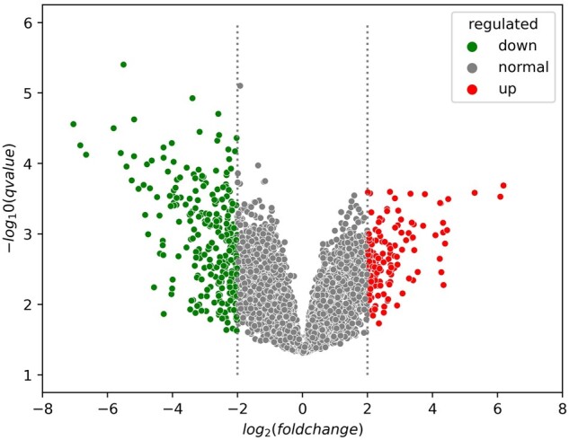
The significant differential expression between kidney cancer and control samples, including up- and down-regulated results
5 Discussion
DeepSec represents the first generalized computational model that can predict secreted proteins in multiple human body fluids. Specifically, this end-to-end model is built based on sequence features extracted via CNN followed by bidirectional GRU. Compared to other models based on proteins features, DeepSec has demonstrated improved prediction accuracy and better generalizability (Fig. 5), which indicates the advantage of sequence-based method as compared to feature-based algorithms. In the blood protein case, the model shows reasonably high AUC (0.94/0.94) and high F-measure (0.91/0.87) on testing dataset and all datasets, as compared to other model architectures (Table 3), which also suggests that DeepSec has good representation of the relevant proteins across the whole protein space.
However, there might be some concerns about the limitations of DeepSec. First, due to the lack of clear knowledge about non-body-fluid secretory proteins, this study generates negative dataset based on Pfam family information. It means that the negative datasets may not adequately include the whole space of the non-body-fluid secretory proteins. Indeed, with larger number of positive instances being identified by wet lab experiments, this model can be better tuned, as demonstrated in Cui et al. (2008). Second, since the protein sequences are compressed into a fixed size vector, there is a risk of information loss. Note that 11.7% (1990 proteins) of human proteins have been influenced by the truncation rule. However, when analyzing the physical properties of those proteins, we understand that the probability of the secreted proteins having long anomic acid sequences is very low, which implies a minimal negative impact on the DeepSec’s performance if there is any. Last, since we addressed the imbalance problem by sampling multiple smaller subsets and recalculates the probabilities based on the same small dataset during the training process, there is a certain likelihood that it introduces risks of overfitting while yielding significantly improved performance. However, when evaluating the performance of DeepSec on all datasets (Table 2), it appears confidently that DeepSec doesn’t overly fit the data.
6 Conclusion
In summary, we propose a DL method, DeepSec, to predict secreted proteins in 12 kinds of human body fluids based on protein sequences. To the best of our knowledge, DeepSec is the first system that fully capture the sequence features related to protein secretion automatically using CNN with BGRU architecture. The BGRU network is able to capture possible long-range dependencies between sequence and secreted status of proteins, which contributes to the improved performance. DeepSec is able to predict the secreted protein with higher accuracy than existing state-of-the-art methods. Moreover, DeepSec is useful for discovering novel candidates of blood biomarkers in kidney cancer that have been experimentally verified. Our future effort will focus on including more types of human body fluids into the system and improve the performance toward biomarker discovery in complex human diseases and physiological phenotypes.
Funding
This work was supported by the National Natural Science Foundation of China [62072212], the Development Project of Jilin Province of China [20200401083GX, 2020C003, 2020LY500L06], Guangdong Key Project for Applied Fundamental Research [2018KZDXM076]. This work was also supported by Jilin Province Key Laboratory of Big Data Intelligent Computing [20180622002JC].
Conflict of Interest: none declared.
Supplementary Material
Contributor Information
Dan Shao, Key laboratory of Symbol Computation and Knowledge Engineering of Ministry of Education, College of Computer Science and Technology, Jilin University, Changchun 130012, China; College of Computer Science and Technology, Changchun University, Changchun 130022, China; Department of Computer Science and Engineering, University of Nebraska-Lincoln, Lincoln, NE 68588, USA.
Lan Huang, Key laboratory of Symbol Computation and Knowledge Engineering of Ministry of Education, College of Computer Science and Technology, Jilin University, Changchun 130012, China.
Yan Wang, Key laboratory of Symbol Computation and Knowledge Engineering of Ministry of Education, College of Computer Science and Technology, Jilin University, Changchun 130012, China; School of Artificial Intelligence, Jilin University, Changchun 130012, China.
Kai He, Key laboratory of Symbol Computation and Knowledge Engineering of Ministry of Education, College of Computer Science and Technology, Jilin University, Changchun 130012, China.
Xueteng Cui, College of Computer Science and Technology, Changchun University, Changchun 130022, China.
Yao Wang, Key laboratory of Symbol Computation and Knowledge Engineering of Ministry of Education, College of Computer Science and Technology, Jilin University, Changchun 130012, China.
Qin Ma, Department of Biomedical Informatics, College of Medicine, The Ohio State University, Columbus, OH 43210, USA.
Juan Cui, Department of Computer Science and Engineering, University of Nebraska-Lincoln, Lincoln, NE 68588, USA.
References
- Altschul S.F. et al. (1997) Gapped BLAST and PSI-BLAST: a new generation of protein database search programs. Nucleic Acids Res., 25, 3389–3402. [DOI] [PMC free article] [PubMed] [Google Scholar]
- Anderson N.L. (2010) The clinical plasma proteome: a survey of clinical assays for proteins in plasma and serum. Clin. Chem., 56, 177–185. [DOI] [PubMed] [Google Scholar]
- Armenteros J.J.A. et al. (2017) DeepLoc: prediction of protein subcellular localization using deep learning. Bioinformatics, 33, 3387–3395. [DOI] [PubMed] [Google Scholar]
- Cui J. et al. (2008) Computational prediction of human proteins that can be secreted into the bloodstream. Bioinformatics, 24, 2370–2375. [DOI] [PMC free article] [PubMed] [Google Scholar]
- Hong C.S. et al. (2011) A computational method for prediction of excretory proteins and application to identification of gastric cancer markers in urine. PLoS One, 6, e16875. [DOI] [PMC free article] [PubMed] [Google Scholar]
- Huang L. et al. (2021) Human body-fluid proteome: quantitative profiling and computational prediction. Brief. Bioinf., 22, 315–333. [DOI] [PMC free article] [PubMed] [Google Scholar]
- Jain A. et al. (2021) Analyzing effect of quadruple multiple sequence alignments on deep learning based protein inter-residue distance prediction. Sci. Rep., 11, 7574. [DOI] [PMC free article] [PubMed] [Google Scholar]
- Lathrop J. et al. (2003) Therapeutic potential of the plasma proteome. Curr. Opin. Mol. Ther., 5, 250–257. [PubMed] [Google Scholar]
- Legrain P. et al. (2011) The human proteome project: current state and future direction. Mol. Cell. Proteomics, 10, M111.009993. [DOI] [PMC free article] [PubMed] [Google Scholar]
- Liang S. et al. (2019) A Novel Matched-pairs feature selection method considering with tumor purity for differential gene expression analyses. Math. Biosci., 311, 39–48. [DOI] [PubMed] [Google Scholar]
- Margolis J., Kenrick K.G. (1969) Two-dimensional resolution of plasma proteins by combination of polyacrylamide disc and gradient gel electrophoresis. Nature, 221, 1056–1057. [DOI] [PubMed] [Google Scholar]
- Nanjappa V. et al. (2014) Plasma Proteome Database as a resource for proteomics research: 2014 update. Nucleic Acids Res., 42, D959–965. [DOI] [PMC free article] [PubMed] [Google Scholar]
- Sara E.G. et al. (2018) The Pfam protein families database in 2019. Nuclc Acids Res., 47, D427–432. [DOI] [PMC free article] [PubMed] [Google Scholar]
- Savojardo C. et al. (2018) DeepSig: deep learning improves signal peptide detection in proteins. Bioinformatics, 34, 1690–1696. [DOI] [PMC free article] [PubMed] [Google Scholar]
- Schwenk J.M. et al. (2017) The human plasma proteome draft of 2017: building on the human plasma PeptideAtlas from mass spectrometry and complementary assays. J. Proteome Res., 16, 4299–4310. [DOI] [PMC free article] [PubMed] [Google Scholar]
- Sun Y. et al. (2015) A computational method for prediction of saliva-secretory proteins and its application to identification of head and neck cancer biomarkers for salivary diagnosis. IEEE Trans. Nanobiosci., 14, 167–174. [DOI] [PubMed] [Google Scholar]
- Thomson J.J. (1914) Rays of positive electricity and their application to chemical analyses. Nature, 92, 549–550. [Google Scholar]
- Tiselius A. (1937) Electrophoresis of serum globulin: electrophoretic analysis of normal and immune sera. Biochem. J., 31, 313–317. [DOI] [PMC free article] [PubMed] [Google Scholar]
- Varland S. et al. (2015) N-terminal modifications of cellular proteins: the enzymes involved, their substrate specificities and biological effects. Proteomics, 15, 2385–2401. [DOI] [PMC free article] [PubMed] [Google Scholar]
- Wang J.X. et al. (2013) Computational prediction of human salivary proteins from blood circulation and application to diagnostic biomarker identification. PLoS One, 8, e80211. [DOI] [PMC free article] [PubMed] [Google Scholar]
- Wang S. et al. (2016a) Protein secondary structure prediction using deep convolutional neural fields. Sci. Rep., 6, 18962. [DOI] [PMC free article] [PubMed] [Google Scholar]
- Wang Y. et al. (2016b) PUEPro: A Computational Pipeline for Prediction of Urine Excretory Proteins. Advanced Data Mining and Applications (ADMA). Gold Coast, QLD, Australia. [Google Scholar]
- Weber M. et al. (2020) Impact of C-terminal amino acid composition on protein expression in bacteria. Mol. Syst. Biol., 16, e9208. [DOI] [PMC free article] [PubMed] [Google Scholar]
- Wilaiprasitporn T. et al. (2020) Affective EEG-based person identification using the deep learning approach. IEEE Trans. Cognit. Dev. Syst., 12, 486–496. [Google Scholar]
- Zhao Y.Y., Lin R.C. (2014) UPLC–MSE application in disease biomarker discovery: the discoveries in proteomics to metabolomics. Chem. Biol. Interact., 215, 7–16. [DOI] [PubMed] [Google Scholar]
Associated Data
This section collects any data citations, data availability statements, or supplementary materials included in this article.