An algorithm for the direct estimation of the parameters of the SIR epidemic model from the I(t) dynamics

Abstract

The discrete SIR (Susceptible–Infected–Recovered) model is used in many studies to model the evolution of epidemics. Here, we consider one of its dynamics—the exponential decrease in infected cases I(t). By considering only the I(t) dynamics, we extract three parameters: the exponent of the initial exponential increase $\gamma$; the maximum value $I_{max}$; and the exponent of the final decrease $\Gamma$. From these three parameters, we show mathematically how to extract all relevant parameters of the SIR model. We test this procedure on numerical data and then apply the methodology to real data received from the COVID-19 situation in France. We conclude that, based on the hospitalized data and the ICU (Intensive Care Unit) cases, two exponentials are found, for the initial increase and the decrease in I(t). The parameters found are larger than reported in the literature, and they are associated with a susceptible population which is limited to a sub-sample of the total population. This may be due to the fact that the SIR model cannot be applied to the covid-19 case, due to its strong hypotheses such as mixing of all the population, or also to the fact that the parameters have changed over time, due to the political initiatives such as social distanciation and lockdown.

Introduction

Among the different models that have been proposed for epidemic evolution, the SIR model is one of the most studied. In its continuous version, it is a system of coupled differential equations indicating the evolution of three quantities: the number of “susceptibles” S(t) of a population corresponding to individuals that can be infected but are not yet infected by a disease; the number of infected people I(t) and the number of recovered people R(t) [1]. In its original and simple version, this model assumes an homogeneous mixing in the population, so that contact is possible between any member of the S population and the I population. The R population has immunity and cannot be infected again.

There is a total of N elements, and the sum of each subpopulation is stable: $S+I+R=N$. The system of evolution equations can be written as:

$$\begin{array}{c}\hfill \begin{array}{cc}\hfill S^{\prime }(t)& =-\beta \frac{S(t)I(t)}{N}\hfill \\ \hfill I^{\prime }(t)& =\left(\beta ,\frac{S(t)}{N},-,\alpha \right)I(t)\hfill \\ \hfill R^{\prime }(t)& =\alpha I(t)\hfill \end{array}\end{array}$$ 1

where $S^{\prime }=dS/dt$, $\beta >0$ and $\alpha >0$ are parameters and $N\gg 1$ is the total size of the population. The parameter $\beta$ characterizes the intensity of the infection, and $\alpha$ the intensity of recovery. Since N, S, I and R have all the same dimension (number of individuals), for the equilibrium of dimensions the parameters $\beta$ and $\alpha$ have both a dimension of 1/time. $T_I=1/\alpha$ is the mean time spent in the I class [2]. In Eq. (1), we can focus only on the first two lines, since the dynamics of $R=N-S-I$ is deduced from the values of S and of I.

This model has been studied in many textbooks and review articles [2–7]. The initial exponential increase in I(t) has been well documented, together with S monotonous decreasing, and R monotonous increasing. However, to our knowledge from studying the literature, the exponential decrease in I(t) has not been closely studied. Here, in the next section, we estimate the coefficient of the exponential decrease, showing that its value is not the same as the initial exponential increase. Using only the I(t) dynamics, and more precisely the two values of the exponential slopes (for increase and decrease) and of the maximum value of I, we further show that all parameters of the SIR model can be estimated numerically. In a further section, we numerically check this procedure and show that all parameters can indeed be estimated with a rather good precision. Finally, we apply this procedure to the COVID-19 pandemic in France, assuming that it corresponds to a SIR model with constant parameters.

Theory

Initial exponential increase in I(t) and its maximum value

First, we will recall how the initial exponential is obtained. This is classical work and is here quickly reviewed.

There is a initial small number of infected people:

$$\begin{array}{c}\hfill I(t=0)=I_0\ll N\end{array}$$ 2

We can also assume that $R=0$ initially, and that $S=N-I-R$ is very close to N, so that initially $S/N\approx 1$. Then, Eq. (1) has the following form for small time periods:

$$\begin{array}{c}\hfill \frac{dI(t)}{I(t)}=(\beta -\alpha )dt\end{array}$$ 3

giving an exponential initial increase for the infected population:

$$\begin{array}{c}\hfill I(t)=I_{0}exp\left[\gamma ,t\right]\end{array}$$ 4

where the exponent is:

$$\begin{array}{c}\hfill \gamma =\beta -\alpha \end{array}$$ 5

The growth rate needs to have $\beta >\alpha$ to have an exponential increase. The following notation is classical, introducing the basic reproduction number $R_0$:

$$\begin{array}{c}\hfill R_0=\frac{\beta }{\alpha }\end{array}$$ 6

so that the condition $\beta >\alpha$ may be written $R_0>1$. When this number is larger than 1, there is an exponential increase in the infected population.

Let us divide the second line of Eq. (1) by its first line. We obtain:

$$\begin{array}{c}\hfill \frac{I^{\prime }}{S^{\prime }}=\frac{\mathit{dI}}{\mathit{dS}}=-1+\left(\frac{\alpha N}{\beta }\right)\frac{1}{S}\end{array}$$ 7

Hence, the evolution of I(S) (time vanished) is the following:

$$\begin{array}{c}\hfill I(S)=-S+\frac{N}{R_0}logS+C\end{array}$$ 8

where C is a constant obtained considering for $t=0$, $I(t)=I_0$ and $S(t)\approx N$. Hence, $C=N+I_0-\frac{N}{R_0}logN$. This then gives, negating the term $I_0/N$ which is very small compared to other terms:

$$\begin{array}{c}\hfill \frac{I(S)}{N}=-\frac{S}{N}+\frac{1}{R_0}log\frac{S}{N}+1\end{array}$$ 9

I first increases, then decreases. The maximum value $I_{max}$ is found for $S=S_{max}=\frac{N}{R_0}$, and we have for $I_{max}$:

$$\begin{array}{c}\hfill \frac{I_{max}}{N}=\frac{1}{R_0}\left(R_0,-,1,-,log,R_0\right)\end{array}$$ 10

The maximum value of the rescaled $I_{max}$ depends only on $R_0$. The curve which is obtained is shown in Fig. 1. We see that it increases nonlinearly with $R_0$.

Fig. 1.

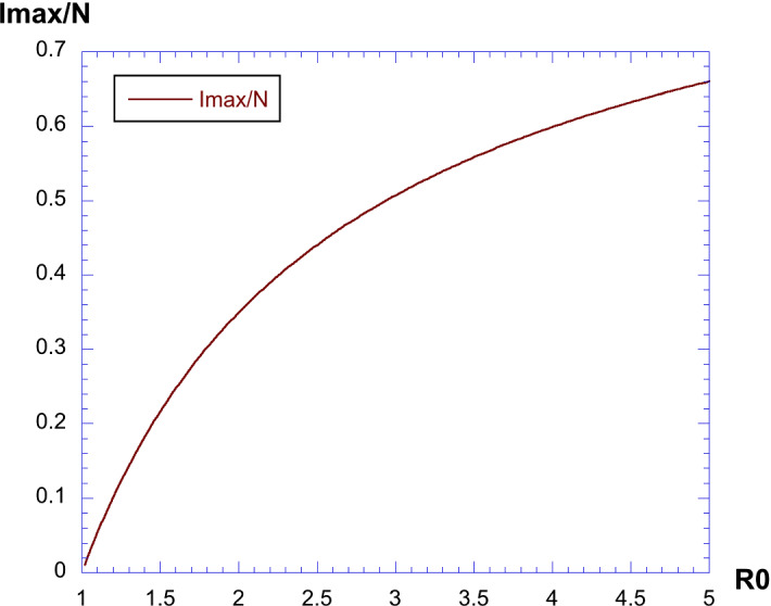
Maximum value of $\frac{I_{max}}{N}$ given by Eq. (10)

The end of the epidemic

We know that at infinite time, we have limit values denoted $S_e$, $I_e$, $R_e$.

By dividing the first line of Eq. (1) by the third line, solving the differential equation obtained, we find finally the evolution of the proportion of S versus R:

$$\begin{array}{c}\hfill \frac{S}{N}=exp\left[-,R_0,\frac{R}{N}\right]\end{array}$$ 11

showing that there is an exponential decrease in susceptible population with respect to the recovered population. We also have:

$$\begin{array}{c}\hfill \frac{S}{N}=exp\left[-,R_0,\frac{R}{N}\right]>exp\left[-,R_0\right]>0\end{array}$$ 12

since $R<N$. This shows that S is decreasing and is minored by a positive value, hence $S_e>0$. An example of dynamics of S(t), R(t) and S(t), chosen for the parameters $I_0=2$, $N=100,000$, $\beta =1.5$ and $R_0=2$ is shown in Fig. 2. This illustrates the fact that $I(t)\to 0$ and $S(t)\to S_e$, as $t\to \infty$. Below we show how $S_e$ can be estimated.

Fig. 2.

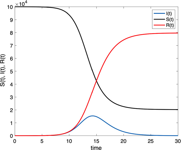
An example of dynamics of S(t), R(t) and S(t), chosen for the parameters $I_0=2$, $N=100,000$, $\beta =1.5$ and $R_0=2$. This illustrates the fact that $I(t)\to 0$ and $S(t)\to S_e$, as $t\to \infty$

First, let us do as in [2], and consider Eq. (1) integrated:

$$\begin{array}{c}\hfill {\int }_0^{\infty }{S}^{\prime }(t)dt=-\frac{\beta }{N}{\int }_0^{\infty }S(t)I(t)dt\end{array}$$ 13

giving:

$$\begin{array}{c}\hfill N-S_e=\frac{\beta }{N}{\int }_0^{\infty }S(t)I(t)dt>\frac{\beta }{N}{S}_e{\int }_0^{\infty }I(t)dt\end{array}$$ 14

This shows that I is integrable, hence for its limit value: $I_e=0$. This corresponds to the end of the epidemic. The corresponding value of $S_e$ can be found by taking $I=0$ in Eq. (9) and is given by:

$$\begin{array}{c}\hfill \frac{S_e}{N}=\frac{1}{R_0}log\frac{S_e}{N}+1\end{array}$$ 15

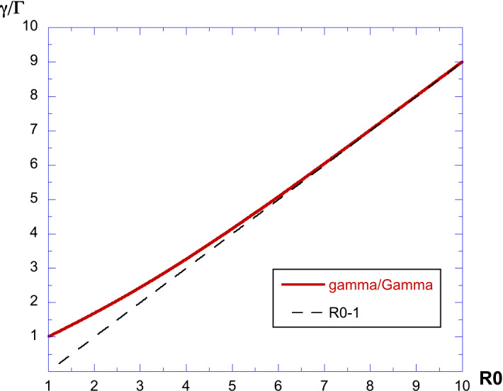
This is an implicit relation providing $S_e/N$ for a given value of the parameter $R_0$. We can consider $1<R_0\le 10$ and solve numerically the implicit relation: find the solution of $f(x)=\frac{1}{R_0}logx+1-x=0$ giving the value of $x=S_e/N$. The result is shown in Fig. 3. Three curves are shown, for $R_0=1.5$, 2 and 2.5. The value of $S_e/N$ is the intersection with the horizontal axis. Doing this numerically for a number of values of $R_0$, we obtain the curves given in Fig. 4 providing $S_e/N$ vs. $R_0$. On the left panel, we show a log-plot, together with the fit $S_e/N=exp\left(-,3.9,(,\sqrt{R_0},-,1,)\right)$. This fit is excellent until a value of $R_0\simeq 4.5$. For $R_0$ large, $S_e/N$ is small.

Fig. 3.

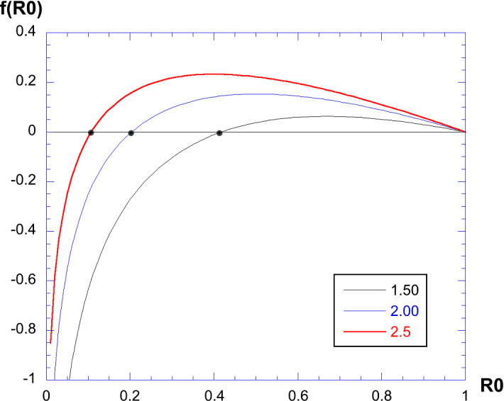
Solving the equation $f(x)=\frac{1}{R_0}log(x)+1-x=0$ for each value of $R_0$: here, three examples with $R_0=1.5$, 2 and 2.5. The intersection of the horizontal axis gives the value of $S_e/N$

Fig. 4.

Solving the equation $log(x)/R_0+1-x=0$ for each value of $R_0$ we have the curve $S_e(R_0)$. Left: linear plot; right: log-linear plot to emphasize the asymptotic exponential curve

When $x\ll 1$, we have $f(x)\simeq \frac{1}{R_0}logx+1$ and hence, the solution of $f(x)=0$ gives $x=S_e/N=exp(-R_0)$. The curve $S_e/N=exp(-R_0)$ is also shown in Fig. 4, we see that it is approximately valid for $R_0\ge 5$.

Since $R+I+S=N$, for the end point for which $I_e=0$ we have $R_e/N+S_e/N=1$; hence, the relative frequency of recovered people $R_e/N$ at the end of the epidemic is $\frac{R_e}{N}=-\frac{1}{R_0}log\frac{S_e}{N}$.

Analytical expression for the decrease in I(t)

This part and the following are the main contributions of the present work. There is no known analytical expression for the behavior of I(t) for all values of t. We know that there is an exponential increase for small values of t, then a maximum, then a decrease in I(t). Considering Eq. (1), we see that when S is approaching its final value $S\simeq S_e$, we have dI/I approaching a constant value proportional to dt:

$$\begin{array}{c}\hfill \frac{\mathit{dI}}{I}\simeq \left(\beta ,\frac{S_e}{N},-,\alpha \right)dt\end{array}$$ 16

Let us introduce the following constant:

$$\begin{array}{c}\hfill \Gamma =-\beta \frac{S_e}{N}+\alpha =\beta \left(\frac{1}{R_0},-,\frac{S_e}{N}\right)\end{array}$$ 17

Hence, we have as a limit law an exponential decrease in I(t) with characteristic exponent $\Gamma$:

$$\begin{array}{c}\hfill I(t)=C{e}^{-\Gamma t};t\gg 1\end{array}$$ 18

where the value of the constant $C>0$ cannot be directly deduced from the SIR model. It is proved in the appendix that $\Gamma >0$ when $R_0>1$ and $\beta >0$.

Using the numerical extraction of $S_e$ for each value of $R_0$, let us plot the curves for the exponents $\gamma /\beta$ and $\Gamma /\beta$. This is shown in Fig. 5. The first exponent is increasing monotonically, whereas the second one reaches a maximum value of ${\Gamma }_{max}\simeq 0.2984$ for $R_{0max}\simeq 2.15$, after which it decreases. Since $\Gamma$ is estimated through a nonlinear and implicit relation between $S_e/N$ and $R_0$, an explicit analytical expression for the values of ${\Gamma }_{max}$ and $R_{0max}$ is not available.

Fig. 5.

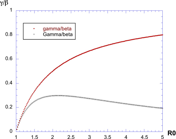
Plot of $\gamma /\beta$ and $\Gamma /\beta$ versus $R_0$. The first exponent is increasing monotonically, whereas the second one reaches a maximum value of 0.2984 for $R_0\simeq 2.15$, after which it decreases. We also see that we have always $\gamma >\Gamma$

We also see that we always have $\gamma >\Gamma$, showing that the two exponents are different as far as $R_0>1$. The shape of I(t) is always asymmetric. To our knowledge, this is the first time the slopes $\gamma$ and $\Gamma$ have been proved to be different and compared for the SIR model.

An algorithm for SIR parameters extraction using only the I(t) curve

From the previous relations, we can propose here an algorithm to extract all SIR parameters only from the infected population dynamics. We assume here that we have experimental data providing the curve I(t) of infected people. This is the easier to measure, since the S population is not clearly defined (say, all the population of a country, or a sub-sample perhaps?). The I(t) curve is typically bell-shaped, with an increasing part, a maximum value and a decreasing part. As seen in the previous section, this curve is asymmetric: it decreases more slowly than it increases, but visually using a linear plot, this asymmetry is not always very clear. Our objective here is, assuming a SIR model, to extract all relevant parameters only from this curve. There are three parameters needed to fully define this model: $R_0$, $\beta$, and N ($\alpha$ is deduced when $R_0$ and $\beta$ are known). Indeed, N is a priori unknown since we do not know what the subsample of the total population is which is interacting homogeneously to obtain the I(t) dynamics. $S_e/N$ will also be a relevant value to be estimated, since it is included in the exponential decrease: it is deduced from the value of $R_0$. Here, we provide a recipe for estimating all these parameters only from the I(t) curve.

(1) The first step is to estimate the coefficient of the exponential increase at the start, $I(t)=I_{0}exp\left[\gamma ,t\right]$. The numerical estimation of the slope $\gamma$ gives:

$$\begin{array}{c}\hfill \gamma =\beta \left(1,-,\frac{1}{R_0}\right)\end{array}$$ 19

The exponential decrease $I(t)=C{e}^{-\Gamma t}$ provides the value of the parameter $\Gamma$:

$$\begin{array}{c}\hfill \Gamma =\beta \left(\frac{1}{R_0},-,\frac{S_e}{N}\right)\end{array}$$ 20

(2) For the second step, $R_0$ is estimated. We consider the ratio $\rho =\gamma /\Gamma$ for which there is no more dependence on the parameter $\beta$:

$$\begin{array}{c}\hfill \rho =\frac{\gamma }{\Gamma }=\frac{R_0-1}{1-R_0\frac{S_e}{N}}\end{array}$$ 21

The ratio depends only on $R_0$ and Se/N, but the latter is related to $R_0$ through a nonlinear relation plotted in Fig. 3, and hence, the $R_0$ value can be estimated from $\rho$ using a nonlinear relationship which is shown in Fig. 6. From the nonlinear relationship represented in this figure, we can deduce the experimental value of $R_0$. When $R_0$ is large, we know from Fig. 4 that $S_e/N\ll 1$, and hence, using Eq. (21) $\rho$ simplifies into:

$$\begin{array}{c}\hfill \rho =R_0-1;R_0\ge 6\end{array}$$ 22

which is also shown in the same figure as an asymptotic relation. In such cases, when $R_0\ge 6$, we simply have $R_0=\rho +1$ (and also $\Gamma =\alpha$; $\beta =\Gamma R_0$) or otherwise $R_0$ is estimated by an interpolation of the plot of this nonlinear curve.

Fig. 6.

Plot of the ratio $\rho =\gamma /\Gamma$: we see an almost linear increase, for values of $R_0$ larger than 6, with an asymptotic value of $R_0-1$ as expected. When the two exponents are known and estimated, this ratio can be used to extract directly the value or $R_0$

(3) From this, using Eq. (19) the value of $\beta =\gamma /(1-\frac{1}{R_0})$ is estimated. From the value of $R_0$, we can also estimate $S_e/N$ using the plot shown in Fig. 3.

(4) A last step is the experimental estimation of the maximum value $I_{max}$ of I(t), which gives the value of N through the following relation:

$$\begin{array}{c}\hfill N=\frac{R_0{I}_{max}}{R_0-1-log{R}_0}\end{array}$$ 23

Results: numerical validation and case study using France’s COVID-19 data

In this section, the above algorithm is applied to two cases: first numerical simulations of the model; and then data from the real world.

Numerical validation of the procedure

In this subsection, numerical simulations are performed in order to check the algorithm which has been proposed here. The simulations are done numerically by running the SIR model with given values for the parameters $\beta$, $\alpha$, $R_0$, and N; choosing an initial value of $I_0$. Subsequently, the algorithm proposed above is applied exclusively on the I(t) curve, in order to consider if the estimated parameters are close to the ones used to perform the simulation. This is a consistency test.

Taking $I_0=2$, $N=100,000$, and different values of $R_0$ and $\beta$, let us first consider $R_0=2.0$ and $\beta =1.5$. Figure 7 shows the evolution numerically of I(t). We see an increase, then a decrease in the curve of infected people. On the right panel, the curve is shown in log-linear plot. Straight lines indicate an exponential initial increase then decrease. We see that the shape is not symmetrical. The decrease is slower than the increase. The values of $\gamma$ and $\Gamma$ are extracted from these curves by a best fit of the exponential law, for the region where straight lines are visible.

Fig. 7.

Plot of I(t) for $I_0=2$, $N=100,000$, $R_0=2.0$ and $\beta =1.5$. Right: a log-linear plot showing the exponential increase and decrease

This has been done keeping $\beta$ constant and varying the value of $R_0$. The result is shown in Fig. 8, in log-linear plot to emphasize the exponential curves, for the value $\beta =1.5$, but other values have of course been tested. All curves have similar behavior, with different time values for the maximum, and also different decrease and increase slopes.

Fig. 8.

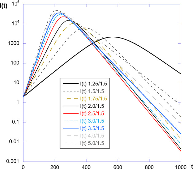
Plot of I(t) for $\beta =1.5$ and different values of $R_0$. We see that all curves have similar behavior, with different time values for the maximum, and also different decrease and increase slopes

Let us now consider the numerical values found for simulations with a fixed value for $\beta$ ($\beta =1.5$, 2 and 3) and values of $R_0$ from 2 to 5. Using the procedure described above, we estimate the value of $I_{max}$, the slopes $\gamma$ and $\Gamma$, their ratio $\rho$, and obtain the value of $R_0$, $\beta$, and N. All the values for the examples shown are visible in Table 1. We see that using this procedure the values of the parameters $R_0$ and $\beta$ are estimated with an error below 1%, and N with an error of a maximum of 5%, and most of the time below 2% . It is also visible that estimated values of $\beta$ and N are very slightly decreasing with increasing values of $R_0$. This numerical test shows that the procedure proposed here is able to extract the correct values of parameters, with a very good precision, probably not accessible from experimental data. In the next section, this procedure is applied to real-world data.

Table 1.

Chosen values for a numerical test of the procedure described in the text. The values of $\beta$, $R_0$, and N are given choices, and the values with ${}^{\ast }$ are numerical estimates. We see that the parameters $\beta$ and $R_0$ are retrieved with a high precision of a maximum of 1 % error, and for N, with an error of a maximum of 5%, and most of the time below 2%

Simulation			Estimation of parameters
$\beta$	$R_0$	N	${\gamma }^{\ast }$	${\Gamma }^{\ast }$	$I_{max}^{\ast }$	${\rho }^{\ast }$	$R_0^{\ast }$	${\beta }^{\ast }$	$N^{\ast }$
1.5	2	${10}^5$	0.747	0.447	15,371	1.672	1.982	1.508	102,270
1.5	3	${10}^5$	0.995	0.412	30,105	2.414	2.974	1.499	101,270
1.5	4	${10}^5$	1.118	0.346	40,418	3.232	3.969	1.495	100,861
1.5	5	${10}^5$	1.193	0.290	47,894	4.111	4.963	1.494	100,677
2	2	${10}^5$	0.993	0.596	15,380	1.665	1.973	2.014	103,400
2	3	${10}^5$	1.320	0.550	30,124	2.400	2.957	1.995	102,060
2	4	${10}^5$	1.482	0.462	40,440	3.208	3.942	1.986	101,530
2	5	${10}^5$	1.578	0.387	47,920	4.077	4.926	1.980	101,260
3	2	${10}^5$	1.488	0.897	15,400	1.659	1.964	3.032	104,680
3	3	${10}^5$	1.978	0.827	30,160	2.393	2.947	2.994	102,610
3	4	${10}^5$	2.222	0.694	40,490	3.203	3.935	2.980	101,810
3	5	${10}^5$	2.368	0.581	47,980	4.075	4.923	2.972	101,410

A test using experimental data from the COVID-19 2020 pandemic

In order to test the proposed procedure from real-world data, and in the framework of the COVID-19 crisis, we have chosen here data from the COVID-19 pandemic in spring 2020 in France. The sources come from the French government (data publicly available from dashboard.covid19.data.gouv.fr). A confinement of the population was effective on March 17, 2020 and lasted for almost 2 months, with a progressive opening of the country beginning on May 11, 2020. The data of March 17 are taken as day 0 in the data reported, and two series are considered consecutively as I curves: first the total hospitalized people due to COVID-19 and then, the total Intensive Care Unit (ICU) people due to COVID-19; both recorded daily. In each case, 100 days are considered.

Let us call $I_H(t)$ the number of hospitalized people, and see if the model described can fit the data. Figure 9 shows the plot of I(t), having the correct shape. We find a maximum value for $t=28$ (April 14), with $I_{H-max}=32,292$. The exponential fits are the following: $exp(0.162T+8.1)$ for the initial increase, and $exp(-0.021T+11.15)$ for the decrease, where T is the time in days. This gives ${\gamma }_H=0.162$ and ${\Gamma }_H=0.021$. Hence, the ratio is ${\gamma }_H/{\Gamma }_H=7.714$ which is very large. We are here in the regime where $\gamma /\Gamma =R_0-1$; hence, $R_{0-H}=8.7$. This gives also ${\beta }_H={\gamma }_H/(1-1/R_{0-H})={\gamma }_H\times 1.13=0.183$. And ${\alpha }_H={\beta }_H/R_{0-H}=0.021$. This means that the mean time in the infected state is 47 days. This large value comes from the fact that the exponential decrease is moderately slow. We also have $S_e/N_H=1.64{10}^{-4}$ and $N_H=1.57I_{H-max}=50709$.

Fig. 9.

Plot of $I_H(t)$ of the total hospitalized people in France due to COVID-19. Left panel: linear coordinates with exponential fits; right panel: log-linear plot with the two fits as straight lines

We then also consider another classification, when the curve I is $I_{\mathit{icu}}$—the number of people in intensive care units (ICU) in France since the beginning of the pandemic. This is shown in Fig. 10, where the double exponential behavior is also found. The two slopes are here ${\gamma }_{\mathit{icu}}=0.16$ and ${\Gamma }_{\mathit{icu}}=0.0346$; and also the value $I_{icu-max}=7148$. We thus obtain ${\gamma }_{\mathit{icu}}/{\Gamma }_{\mathit{icu}}=4.62$, which is quite large again. This gives $R_{0-icu}=5.52$. We conclude with the following values: ${\beta }_{\mathit{icu}}={\gamma }_{\mathit{icu}}\times 1.22=0.195$, ${\alpha }_{\mathit{icu}}=0.0354$ giving a mean residence time of ICU state of 28 days; and also $N_{\mathit{icu}}=1.96\times I_{icu-max}=14000$.

Fig. 10.

Plot of $I_{\mathit{icu}}(t)$ of people in intensive care unit in France due to COVID-19. Left panel: linear coordinates; right panel: log-linear plot. The log-linear plot shows two exponential behavior

Discussion

About the $R_0$ estimation and its values found in previous works devoted to COVID-19

For a given epidemic situation, the basic reproduction number $R_0$ can be defined independently of the model considered: it is the average number of secondary cases in the infected population [8, 9]. The significance and estimation of the basic reproduction number is a matter of great interest [8–13]. This number is difficult to measure directly and is a complex metric [13].

We have shown here how to obtain it directly in the framework of the SIR model, when the infection curve dynamics is known. $R_0$ is directly and precisely estimated from the ratio $\rho =\gamma /\Gamma$ of initial and final exponential slopes of I(t). The estimation has been shown to be quite precise. Other methods have been proposed to extract $R_0$: first, $\alpha$ can be estimated as the inverse of the mean residence time in the infected situation for a given individual. However, this method requires the information about the situations of a large number of individuals, which is not always the case or possible. Next, parameters are extracted by performing a “best fit,” guessing first some values, and then performing an optimization through a nonlinear fit [2]. Other more complex methods define a next-generation operator and extract $R_0$ from the eigenvalues of this operator [11, 14].

Since the outbreak of the COVID-19 pandemic in China late 2019, a huge number of works have been submitted and published: in March 2020, there were already 500 papers in the press [15]. Among them, many have been devoted to applying the SIR model to different cities or countries: to several countries [16]; to Wuhan administrative region [17]; to Italy [18]; to Brazil [19]; among others. Other variants have also been proposed, such as the SEIR model for the USA [20], or the stochastic SIR model [21].

Very early in the COVID-19 outbreak, some papers have tried to estimate $R_0$. For example, there is a highly cited work that was accepted at the end of January 2020, and since published, that estimated the value of $R_0$ from Wuhan data, using Laplace transform of a function, which is modeled in an ad hoc way, assuming a Gamma probability density function [22]. This work proposes values of $R_0$ from 2.24 to 3.58, but the important role of the assumptions should not be forgotten. There are other works that have proposed some basic fits of the exponential initial growth of the epidemic and found values of, e.g., 3.1 for Italy [23] or 4.5 for France [24]. Concerning France, some other works have already addressed the French COVID-19 pandemic outbreak and the estimation of $R_0$: see, e.g., [25, 26], where values from 1.7 to 4.2 have been reported.

Some papers have proposed meta-analysis of published works. For example, [27] considered as early as February 7, 2020, 12 studies and found values of $R_0$ ranging from 1.4 to 6.49, obtained using methods varying from the stochastic Markov chain model and SEIR to compartmental models and stochastic simulations. The same type of work was done in March, 2020, concerning 23 studies that found $R_0$ values ranging from 1.9 to 6.49 [28].

About the relatively large values of $R_0$ found using our algorithm

We see that ordinarily when a SIR or a similar model is used, the nonlinear fits—other complicated methods—are employed on the growth part but do not use the information provided by the decreasing part of the infection curve. Our argument here is that both of these should be considered, as they are part of the same dynamics. But of course, in our method, we need to assume (1) that the SIR model is the correct one to model the pandemic and (2) that parameters have not changed in time. Indeed the initiative of political authorities has been, all around the world, trying to decrease $R_0$ by social distancing and sometimes lockdown of the population during weeks or months. These political decisions may change the parameters of the model and correspond to limits in the application of our method.

Using our algorithm, we have found two different $R_0$ values. First, by considering the hospitalized population (due to COVID-19) in France, we found $R_{0-H}=8.7$, ${\beta }_H=0.183$, ${\alpha }_H={\beta }_H/R_{0-H}=0.021$, and $N_H=50709$. This is found assuming that this SIR model is valid to describe the $I_H$ dynamics, and that the parameters have not changed during the lockdown. With this assumption, we find a SIR model with quite a large $R_0$ value and a susceptible population (S value), initially around 50,000 people, far from the about 67 million approximate population of France. Let us recall that this model assumes a homogeneous mixing of the infected and susceptible populations. This means that this model could work here, if we consider only a sub-population who are concerned with being in contact with the infected population.

The second set of values was found by applying the model to the section of the infected population who were put in intensive care units (ICU). Let us recall that the lockdown was decreed in France (as in other countries such as China, Italy, and Spain, at that time) by the French government in order to maintain the number of ICU at a given limit (5000 at the time), and avoid loosing control of the situation in hospitals. In this framework, to consider the SIR model with I being the ICU part of infected people, has some justification. Then, the S part of the population is here the hospitalized population: they are susceptible to going from the hospitalized state to the ICU state. Using the algorithm, we found $R_{0-icu}=5.52$, ${\beta }_{\mathit{icu}}=0.195$, ${\alpha }_{\mathit{icu}}=0.0354$, and $N_{\mathit{icu}}=14,000$. This means that, if this model is correct and if the parameters have not changed during the 100 days of the study, there were 14,000 susceptible people that could have gone to the ICU state. We also remark that the two estimates of $\beta$ are quite close, whereas for $\alpha$ there is a difference, and the mean duration for an individual in the H-state is $T_H=1/{\alpha }_H=47$ days, whereas $T_{\mathit{icu}}=1/{\alpha }_{\mathit{icu}}=28$ days. These numbers seem realistic and translate the fact that the decreasing exponentials are rather slow. There is a long memory in both curves.

Are such large values of $R_0$ realistic? First, let us note that in their review, Delamater et al. [13] mention relatively large values of $R_0$, going from 12.5 for measles in the USA (1912–1928); 13.7 to 18 for measles again in England and Wales in 1944-1979; and values of 12 to 17 for pertussis in England Wales and the USA in the same periods. The values found here for COVID-19 in France are much lower.

Furthermore, it has been already mentioned that there is a higher contact rate for high density population [29]. This may also be supported by recalling that in Eq. (1) the coefficient $\beta$ corresponds to a contact rate between the S and I populations. In the field of turbulent particle dynamics (which could be an analogy with human movements in an active society), when there is a large concentration of particles, it has been shown that the contact rate is multiplied by a new factor corresponding to this accumulation, and that this factor can be as large as 10 [30, 31]. This means that when there is an accumulation of particles, the contact rate increases with a factor that can be explained and modeled. It is known that human population is not uniform in space; there are large inhomogeneities in human population density, in a way which has been characterized as multifractal, i.e., highly concentrated: see, e.g., [32] for an analysis of the French population density. Such accumulation may explain the large values for the contact rate, and hence, the large value of $R_0$ found here.

However, associated with this large $R_0$ value is the fact that the N population is rather limited, meaning that most of the population is not concerned with the risk of infection: there is a huge concentration of the transmission from a limited number of infected people to an also limited number of susceptible people.

Finally, we need to emphasize again that this application to real-world data is valid only on the hypothesis that the SIR model is correct and has constant parameters.

Conclusion and perspectives

The algorithm proposed here in the framework of the SIR epidemic model needs to know the maximum value of the infected population $I_{max}$, the exponential slope for the initial increase $\gamma$ and the exponential slope of the final decrease in the I dynamics $\Gamma$. From these three empirical estimations, we first compute the ratio $\rho =\gamma /\Gamma$ and from it, using a nonlinear curve, the basic reproduction number $R_0$ is directly estimated. From $R_0$ and $\gamma$, the value of $\beta$ is extracted, as well as the $\alpha$ parameter. Then, the total number N corresponding to the initial susceptible population $S_0$ is estimated from $I_{max}$ and $R_0$.

This algorithm has been tested using different values of the parameter $R_0$. It has also been applied to a situation of real-world data, for the COVID-19 situation in France. The value of $R_0$, which was found to be 8.7 for the hospitalized population and 5.52 for the ICU population, is larger than other estimates where $R_0$ is between 2 and 3. However, this may be linked with the applicability of the SIR model, since our data analysis is valid only for this model. What has been shown, is that, if the SIR model can be applied to the COVID-19 infectious dynamics in France, with fixed values of its parameters, then the $R_0$ value is relatively large. It may be that the lockdown had changed the behavior of the population, and that the parameters had changed over time. Other more complex models than the SIR may also be applied to these real-world data, e.g., taking into account the stratification of the population, SIR model with time changing parameters, or the heterogeneity of the population. The quality of the experimental data is also an issue. Indeed, real data of infected and recovered people are hugely biased, since, e.g., many people have been infected and then recovered without leaving any record. There is a large uncertainty in the application of statistical physics to societal phenomena, including epidemics measurements.

Let us finally remark that in the SIR model the decline of the epidemics depends on the depletion of the susceptible population. At the scale of a country, this decline is possible either by limiting the contacts between individuals, so that the total concerned individuals N is much smaller than the total population of the country. Another approach, done in 2021 all over the world, is to diminish the susceptible population through the vaccination.

The perspectives of this work may be to extend the approach to other famous epidemic models, such as the SEIR (where another state is introduced—the “exposed” population, which is infected but not infectious). This introduces a delay in the dynamics, and the calculation performed here would need to be revised.

Appendix: Proof of $\Gamma >0$

In this appendix, we prove the following theorem: $\Gamma =\beta \left(\frac{1}{R_0},-,\frac{S_e}{N}\right)>0$ when $\beta >0$ and $R_0>1$.

Proof

Since $\Gamma =\beta \left(\frac{1}{R_0},-,\frac{S_e}{N}\right)$, the condition $\Gamma >0$ is equivalent to state that $1/R_0>S_e/N$. The value of $S_e/N$ is the solution $0<x<1$ of:

$$\begin{array}{c}\hfill \frac{1}{R_0}logx+1-x=0\end{array}$$ 24

We need to show that this solution verifies $R_{0}x<1$.

It is a standard relation to consider that one has for $y>-1$ [33]:

$$\begin{array}{c}\hfill \frac{y}{1+y}\le log(1+y)\le y\end{array}$$ 25

By writing $x=1+y$, we have for $x>0$:

$$\begin{array}{c}\hfill \frac{x-1}{x}\le logx\end{array}$$ 26

Using Eq. (24), we have:

$$\begin{array}{c}\hfill \frac{x-1}{x}\le R_0(x-1)\end{array}$$ 27

Since $x-1<0$, this gives $R_0\le \frac{1}{x}$.

We still need to exclude the equality $R_{0}x=1$. For this, let us note that if $R_{0}x=1$, inserting $x=1/R_0$ in Eq. (24) gives an equation for $R_0$: $-log{R}_0+R_0-1=0$. Its only solution is $R_0=1$. Since we assume here that $R_0>1$, we may write that $R_{0}x\ne 1$.

Hence, it is proved that $R_{0}x<1$, implying $\Gamma >0$. $\square$

References

- 1.Kermack WO, McKendrick AG. Proc. Royal Soc. London Series A. 1927;115(772):700. [Google Scholar]
- 2.Martcheva M. An Introduction to Mathematical Epidemiology. New York: Springer; 2015. [Google Scholar]
- 3.Hethcote HW. SIAM Rev. 2000;42(4):599. doi: 10.1137/S0036144500371907. [DOI] [Google Scholar]
- 4.Daley DJ, Gani J. Epidemic Modelling: An Introduction. Cambridge: Cambridge University Press; 2001. [Google Scholar]
- 5.Brauer F. Math. Biosci. 2005;198(2):119. doi: 10.1016/j.mbs.2005.07.006. [DOI] [PubMed] [Google Scholar]
- 6.Murray JD. Mathematical Biology: I An Introduction. Berlin: Springer; 2007. [Google Scholar]
- 7.Breda D, Diekmann O, De Graaf W, Pugliese A, Vermiglio R. J. Biol. Dyn. 2012;6(sup2):103. doi: 10.1080/17513758.2012.716454. [DOI] [PubMed] [Google Scholar]
- 8.Heesterbeek J, Dietz K. Stat. Neerlandica. 1996;50(1):89. doi: 10.1111/j.1467-9574.1996.tb01482.x. [DOI] [Google Scholar]
- 9.Breban R, Vardavas R, Blower S. PLoS One. 2007;2(3):e282. doi: 10.1371/journal.pone.0000282. [DOI] [PMC free article] [PubMed] [Google Scholar]
- 10.Dietz K. Stat. Methods Med. Res. 1993;2(1):23. doi: 10.1177/096228029300200103. [DOI] [PubMed] [Google Scholar]
- 11.Heesterbeek JAP. Acta Biotheor. 2002;50(3):189. doi: 10.1023/A:1016599411804. [DOI] [PubMed] [Google Scholar]
- 12.Wallinga J, Lipsitch M. Proc. Royal Soc. B: Biol. Sci. 2007;274(1609):599. doi: 10.1098/rspb.2006.3754. [DOI] [PMC free article] [PubMed] [Google Scholar]
- 13.Delamater PL, Street EJ, Leslie TF, Yang YT, Jacobsen KH. Emerg. Infect. Dis. 2019;25(1):1. doi: 10.3201/eid2501.171901. [DOI] [PMC free article] [PubMed] [Google Scholar]
- 14.Diekmann O, Heesterbeek JAP, Metz JA. J. Math. Biol. 1990;28(4):365. doi: 10.1007/BF00178324. [DOI] [PubMed] [Google Scholar]
- 15.Callaway E, Cyranoski D, Mallapaty S, Stoye E, Tollefson J. Nature. 2020;579:482. doi: 10.1038/d41586-020-00758-2. [DOI] [PubMed] [Google Scholar]
- 16.Toda AA. Covid Econ. 2020;1:43. [Google Scholar]
- 17.Roda WC, Varughese MB, Han D, Li MY. Infect. Dis. Modell. 2020;5:271. doi: 10.1016/j.idm.2020.03.001. [DOI] [PMC free article] [PubMed] [Google Scholar]
- 18.G.C. Calafiore, C. Novara, C. Possieri, 2020 59th IEEE Conference on Decision and Control (CDC) pp. 3889–3894 (2020)
- 19.Bastos SB, Cajueiro DO. Sci. Rep. 2020;10:19457. doi: 10.1038/s41598-020-76257-1. [DOI] [PMC free article] [PubMed] [Google Scholar]
- 20.A. Atkeson, What will be the economic impact of COVID-19 in the us? Rough estimates of disease scenarios (Tech. rep, National Bureau of Economic Research, 2020)
- 21.A. Simha, R.V. Prasad, S. Narayana, arXiv preprint arXiv:2003.11920 (under submission) (2020)
- 22.Zhao S, Lin Q, Ran J, Musa SS, Yang G, Wang W, Lou Y, Gao D, Yang L, He D, et al. Int. J. Infect. Dis. 2020;92:214. doi: 10.1016/j.ijid.2020.01.050. [DOI] [PMC free article] [PubMed] [Google Scholar]
- 23.M. D’Arienzo, A. Coniglio, Biosaf. Health 2, 57 (2020) [DOI] [PMC free article] [PubMed]
- 24.Liu Z, Magal P, Webb G. J. Theor. Biol. 2020;509:110501. doi: 10.1016/j.jtbi.2020.110501. [DOI] [PMC free article] [PubMed] [Google Scholar]
- 25.J. Roux, C. Massonnaud, P. Crépey, medRxiv (under submission) (2020)
- 26.Roques L, Klein EK, Papaix J, Sar A, Soubeyrand S. Front. Med. 2020;7:274. doi: 10.3389/fmed.2020.00274. [DOI] [PMC free article] [PubMed] [Google Scholar]
- 27.Y. Liu, A.A. Gayle, A. Wilder-Smith, J. Rocklöv, J. Travel Med. 27, taaa021 (2020) [DOI] [PMC free article] [PubMed]
- 28.Alimohamadi Y, Taghdir M, Sepandi M. J. Prev. Med. Public Health. 2020;53:151. doi: 10.3961/jpmph.20.076. [DOI] [PMC free article] [PubMed] [Google Scholar]
- 29.Hu H, Nigmatulina K, Eckhoff P. Math. Biosci. 2013;244(2):125. doi: 10.1016/j.mbs.2013.04.013. [DOI] [PubMed] [Google Scholar]
- 30.Sundaram S, Collins LR. J. Fluid Mech. 1997;335:75. doi: 10.1017/S0022112096004454. [DOI] [Google Scholar]
- 31.Wang LP, Wexler AS, Zhou Y. Phys. Fluids. 1998;10(10):2647. doi: 10.1063/1.869777. [DOI] [Google Scholar]
- 32.Sémécurbe F, Tannier C, Roux SG. Geogr. Anal. 2016;48(3):292. doi: 10.1111/gean.12099. [DOI] [Google Scholar]
- 33.Love ER. Math. Gaz. 1980;64(427):55. doi: 10.2307/3615890. [DOI] [Google Scholar]