

Abstract
The major oil fields are currently in the middle and late stages of waterflooding. The water channels between the wells are serious, and the injected water does little effect. The importance of profile control and water blocking has been identified. In this paper, the decision-making technique for water shutoff is investigated by the fuzzy evaluation method, FEM, which is improved using a random forest, RF, classification model. A machine learning random forest algorithm was developed to identify candidate wells and to predict the well performance for water shutoff operation. A data set consisting of 21 production wells with three-year production history is used, where out of the mentioned well data, 70% of them are implemented for training and the remaining are used for testing the model. After fitting the model, the new weights for the factors are established and decision-making is made. Accordingly, 16 wells out of 21 wells are selected by the FEM where 8 wells out of 21 wells are selected by the new factor weight created by RF for water shutoff. A numerical simulation model is established to plug the selected wells by both methods after which the influence of plugging on water cut, daily oil production, and cumulative oil production is compared. The paper shows that the reservoir had a better performance after eight wells were selected using a new weighting system created by RF instead of the 16 wells that were selected using the FEM model. The paper also states that the new weighting model’s accuracy improved the decision-making abilities of the wells.
1. Introduction
The world’s oil reserves are widely dependent on the exploitation and production of these resources. The various economic sectors rely on these commodities for their growth. The management of these reserves is one of the most critical factors that can affect the profitability of the oil industry.1 As the oil reservoir’s production rate is gradually declining, enhanced oil recovery (EOR) techniques are becoming more prevalent in the oil industry. These techniques can help maintain the reservoir’s production capacity.2,3
It is very simplistic to judge the need for plugging an oil well based on the water cut.4 From a block perspective, when multiple oil wells produce water at the same time, due to different reasons for water discharge, not every water well needs to be blocked. Thus, systematic well selection is required. The traditional method of blindly selecting wells based on experience sometimes exacerbates the water production of other oil wells and worsens the water production of oil wells throughout the block.5 Hence, there is an urgent need to develop an accurate and simple well plugging method. A water shutoff system entirely extracts the remaining oil and can effectively enhance oil recovery.6,7 A series of decision-making systems are required for water shutoff in one way to utilize the maximum possible remaining oil and in another way to facilitate the procedure for optimization.8
There are two main methods for selecting wells for plugging. One is through qualitative analysis using the field experience,9 while the other is with decision-making existing software. The fuzzy math decision-making method is a commonly used method in the oil and gas industry. It involves using a series of indicators to make well selection decisions.10−12 The key component of the method is the weight factor calculation.13 Liu et al.14 utilized the software called RS to optimize multiple well profile controls and water shutoff treatments. This software combines reservoir engineering and numerical modeling to provide a simple and efficient way to select and optimize wells.13
The fuzzy clustering algorithm is a type of data collection method that was used by Jiang et al.15 for early warning well selection decisions. This study presents an improved fuzzy clustering algorithm that can provide better results in terms of reducing the objective functions. During the high water cut stage, wells with similar characteristics can be tuned to have a profile. The clustering algorithm can then be used to identify the similarities among different types of wells. Xia et al.8 present a clustering model that can be used to select well candidates for plugging to the actual oilfield. Li16 has used the theory of solving matrix in the fuzzy mathematics method to solve statistical weighting.17,18 The pressure index decision-making technique was used by Wang19 and other researchers to evaluate the candidate well selection that they need for plugging or not.20−22 The technique was developed using the transient well test theory. Generally, well selection can be done by analyzing the well bore problem, well bore evaluation, and decision-making techniques.23
In this paper, first, the candidate wells are selected for water shutoff through the fuzzy evaluation method, FEM, and the decision-making technique has been established. In the FEM, the factors affecting the judgment of well plugging have been created. The weight system for the created factors has been considered. To achieve the decision-making for a well-plugging result, the evaluation set has been made. Determination of the weight of each factor, which is a significant part of the calculation, can be a great challenge in the FEM. In the FEM, there is no sufficient mechanism to calculate the accurate weighting system for each factor. In this method, the factor weight will be taken subjectively. As weight is an important part of this evaluation, it will heavily influence the final decision-making result. Thus, the results of well selection of this kind of weighting system can be inaccurate.
In order to increase the correctness of well selection decision-making, the machine learning random forest RF algorithm is used to create a high-accuracy factor weight. In the RF calculation, the same factors used in the fuzzy evaluation method (FEM) are considered as features and the decision result obtained from this calculation is used as a label. In a machine learning RF algorithm, the weight of the factors can be calculated and a high-accuracy weighing system may be provided. As the weighting system is provided by the machine, it could be accurate. Using the RF algorithm, the factors are improved by the historical production data of each well.
In the last part of this paper, a numerical simulation study is considered to verify the new method contrast. The actual production rate of three simulated models is compared by a numerical simulation. A base model that has no wells are selected for plugging and normally the production process is resumed until 2040; 16 wells selected by the FEM are plugged models, and 8 wells selected by the weight of new factor created by the RF model are plugged. Finally, the weight calculation method proposed in this paper is compared with the entropy method presented by Weiguo and Gichong24 in 2009.
2. Materials and Methods
In this paper, the random forest (RF) machine learning method is selected to create the factor weight in order to develop the decision-making of production wells for water shutoff. In RF, the same factors, the pressure build-up decision-making factor value (PBD), rising index of oil well water cut (WI), and residual oil saturation (Sor), used in the fuzzy evaluation method (FEM) were considered as variables and the outcome obtained from the FEM was measured as a label. The purpose of using this algorithm is to generate a new factor weight, so it can enhance the accuracy of the decision-making of well selection. The result achieved by the FEM can be inaccurate; however, using RF, the machine will calculate the importance of the features. As the factor weight or the feature importance is a part of the calculation, it will definitely affect the final result. In machine learning beyond the methods, preparing a result can be more complicated in order to apply it to the oil and gas field.25 Through the random selection of both the input data and the variables, the RF is able to generate decision trees. During the prediction procedure, those features that do not imply any significance of the final result can be ignored.26
Figure 1 illustrates the creation process of the new factor weight by the RF classification model for a decision-making study. The process starts from establishing a factor, creating a weight set, to creating an evaluation set through the FEM. Using the FEM, a comprehensive evaluation is conducted and decision-making is established. The next step is using RF to create a new weight for the factors of each well. To achieve an accurate weight result for each well, the historical production of the wells is also used. The production history data of 3 years are used for this calculation. The PBD, WI, and Sor values are created for 36 months by using geologic and production data provided from the oilfield. The well selection results are determined for each month by the FEM. By using this monthly result and the factor value, the new factor weight is calculated by RF as shown in Table 2.
Figure 1.

Diagram of factor weight creation and the decision-making procedure of the RF model.
Table 2. PBD, WI, and Sor Using Production History for One Well, Well L13-19.
| Well-ID | date | PBD | WI | Sor | remark |
|---|---|---|---|---|---|
| L13-19 | 1/31/2017 | 0.33 | 0.99 | 0.40 | selected for water shutoff |
| L13-19 | 2/28/2017 | 0.32 | 0.99 | 0.40 | selected for water shutoff |
| L13-19 | 3/31/2017 | 0.37 | 0.99 | 0.40 | not selected for water shutoff |
| L13-19 | 4/30/2017 | 0.35 | 0.97 | 0.40 | selected for water shutoff |
| L13-19 | 5/31/2017 | 0.38 | 0.98 | 0.39 | not selected for water shutoff |
| L13-19 | 6/30/2017 | 0.35 | 0.98 | 0.39 | selected for water shutoff |
| L13-19 | 7/31/2017 | 0.36 | 0.96 | 0.39 | selected for water shutoff |
| L13-19 | 8/31/2017 | 0.39 | 0.92 | 0.39 | selected for water shutoff |
| L13-19 | 9/30/2017 | 0.39 | 0.95 | 0.39 | not selected for water shutoff |
| L13-19 | 10/31/2017 | 0.38 | 0.95 | 0.39 | not selected for water shutoff |
| L13-19 | 11/30/2017 | 0.35 | 0.97 | 0.39 | selected for water shutoff |
| L13-19 | 12/31/2017 | 0.36 | 0.97 | 0.39 | selected for water shutoff |
| L13-19 | 1/31/2018 | 0.36 | 0.98 | 0.39 | not selected for water shutoff |
| L13-19 | 2/28/2018 | 0.32 | 0.99 | 0.39 | selected for water shutoff |
| L13-19 | 3/31/2018 | 0.36 | 0.99 | 0.39 | not selected for water shutoff |
| L13-19 | 4/30/2018 | 0.36 | 0.99 | 0.39 | not selected for water shutoff |
| L13-19 | 2/28/2019 | 0.36 | 0.99 | 0.38 | not selected for water shutoff |
| L13-19 | 3/31/2019 | 0.36 | 0.99 | 0.38 | not selected for water shutoff |
| L13-19 | 4/30/2019 | 0.35 | 0.98 | 0.38 | selected for water shutoff |
| L13-19 | 5/31/2019 | 0.36 | 0.99 | 0.38 | not selected for water shutoff |
| L13-19 | 6/30/2019 | 0.35 | 0.99 | 0.38 | not selected for water shutoff |
| L13-19 | 7/31/2019 | 0.35 | 0.99 | 0.38 | not selected for water shutoff |
| L13-19 | 8/31/2019 | 0.34 | 0.99 | 0.38 | selected for water shutoff |
| L13-19 | 9/30/2019 | 0.36 | 0.99 | 0.39 | not selected for water shutoff |
| L13-19 | 10/31/2019 | 0.36 | 0.99 | 0.39 | not selected for water shutoff |
| L13-19 | 11/30/2019 | 0.36 | 0.99 | 0.39 | not selected for water shutoff |
After obtaining the new weight results from the RF algorithm, the comprehensive evaluation is applied to them and a final decision-making result has been conducted. The four stages considered in this study are as follows: (1) the preparation of the dataset for the FEM, (2) prediction of the data by RF, (3) computation of the factor weight (feature importance), and (4) comprehensive evaluation of weight and factors in order to get the final decision result. Based on the calculated parameters, the factors’ data, and the decision-making result by the FEM, a table is created in an MS Excel format as illustrated in Table 2. The data table contains three indicators, PBD, WI, and Sor values, used as features, while the decision-making result via the FEM is used as a label (remark). For calculations, the Python environment has been chosen. The choice of Python has been based on its extensive capabilities for working with data arrays as matrices, provided by the NumPy library.27 To work on exporting and importing data to the MS Excel format, the Pandas library has been used.28,29 RF uses the implementation of scikit-learn.30,31 The performance of the libraries used fell within the requirements of the “on-demand” computing time. These calculations have been performed on a 64-bit windows PC.
2.1. Decision-Making by the FEM
In the FEM, to make a comprehensive decision, the index parameters should be normalized, the degree of membership is introduced to represent the size of each decision factor, and the membership function is selected using a trapezoidal distribution.12,14,15,19,32 The greater the value of residual oil saturation Sor and oil well water cut index WI, the more the oil wells need to be plugged. Thus, the above two factors are selected to be expressed as a half-trapezoid distribution. The oil wells with a larger pressure build-up value, PBD, do not need to block water, so they are expressed by a half-trapezoidal distribution.16
2.1.1. Establishing Factor Sets
A set of three factors that affect the choice of water blocking of production wells are considered as follows:
| 1 |
In the formula, PBD is the pressure build-up decision-making factor, WI is the rising index of oil well water cut, and -Sor is the residual oil saturation.
From Horner’s33 analysis method for the pressure build-up well test, eq 2 was obtained as follows.
| 2 |
In the formula, Pws (t) is the bottom hole pressure at the time of closing the well, MPa; Pi is the bottom hole pressure, i is infinite shut-in time, MPa; q is the oil well output, m3/d; μ is the underground crude oil viscosity, mPa·s; K is the oil absolute permeability of the reservoir, μm2; h is the effective thickness of the oil layer, m; T is the stable production time of the oil well, h.
Taking Pws (t) as
the ordinate,  is the x axis, and a semi-log
Horner curve is obtained, whose slope is k and the
intercept is Pi. In 1956, Perrine34 proposed the pressure theory to describe the
multiphase flow law of water-filled reservoirs. The concept of the
two-phase fluid flow law is the same as the single-phase flow law.
When the oil well is shut in for a short time, the bottom hole pressure
drop can be replaced by the actual pressure drop. This eliminates
the need for the skin effect calculation as the following eq 3.
is the x axis, and a semi-log
Horner curve is obtained, whose slope is k and the
intercept is Pi. In 1956, Perrine34 proposed the pressure theory to describe the
multiphase flow law of water-filled reservoirs. The concept of the
two-phase fluid flow law is the same as the single-phase flow law.
When the oil well is shut in for a short time, the bottom hole pressure
drop can be replaced by the actual pressure drop. This eliminates
the need for the skin effect calculation as the following eq 3.
 |
3 |
In the formula, Pwf (0) is the instantaneous bottom hole pressure in the closed well, MPa; λt is the sum of the fluidity of the two-phase fluid, μm2/(mPa·s); η is the function of the boundary effect of a well and of the production time; ϕ is the porosity of the reservoir, decimal; Ct is the effective elastic compression coefficient, MPa–1; rw is the radius of the oil well, m; B is the ground layer volume coefficient, m3/m3.
 |
4 |
In the formula, fw is the water content, decimal; qw and qo are the water flow and oil flow through the cross-sectional area of the seepage through the rock layer, m3/d, respectively; Kw and Ko are the effective permeability of the water phase and the oil phase, μm2, respectively; μw and μo are the viscosity of formation of water and oil, mPa·s, respectively; Krw and Kro are the relative permeability of the water phase and the oil phase, μm2, respectively. From eq 4, the oil relative permeability is obtained as follows.
| 5 |
The pressure build-up decision-maker factor or PBD is a decision index that shows the properties of the fluid and the formation. It can be obtained by combining the formation and recovery curve values.
| 6 |
 |
7 |
| 8 |
In the formula, PBD is the pressure build-up decision-making factor. The PBD value is inversely proportional to the water permeability, inversely proportional to the effective thickness of the formation, inversely proportional to the fluidity of water, and inversely proportional to the coefficient hKw. The PBD value can be used to select oil wells that need to be blocked.
From the water cut curves of each oil production well, the definite integral is solved according to the relevant calculation software, and the WI value of each oil well is calculated. The larger the WI value is more water plugging measures are required for the corresponding oil production well. Oil well water cut rise index is calculated based on eq 9.
| 9 |
where WI is the water cut index of the oil well, fw (t) is the function of the water cut of the oil well over time, and t is time.
2.1.2. Creating a Weight Set
Different factors have different importance for the selection of water blocking wells, so different factor weights are assigned to represent the importance of the influence of each factor on the selection of water blocking wells.
| 10 |
In the formula, A is the weight set and ai represents the corresponding weight of each factor (i = 1, 2, ..., n; n is the dimension of the factor). The weight of each factor should meet
| 11 |
In the selection process of water plugging wells, a high residual oil saturation Sor value is the most important prerequisite for water plugging oil wells. The rising water cut index WI is related to the urgency of water plugging oil wells, and the PBD value is a reference indicator for the selection of water plugging oil wells.
2.1.3. Creating Evaluation Set
For the single-factor evaluation set, the following equations are considered:
| 12 |
In eq 12, rij is the evaluation value of each factor (i = 1, 2, ..., n and j = 1, 2, ..., m; n and m are integers. m is the number of factor and n is the dimension of the factor.)
The single factor evaluation matrix is as follows:
 |
13 |
The comprehensive evaluation set B is the product of the weight set A and the evaluation matrix R.
 |
14 |
In the formula, Bi is the comprehensive evaluation value of each evaluation factor, that is, the comprehensive decision value of the oil well. The comprehensive decision-making average value B̅ of the oil well is obtained by the following formula:
| 15 |
2.1.4. Application of the FEM on the North Liuzan Oilfield
2.1.4.1. The North Liuzan Block
The north Liuzan block is a layered fault-block oil reservoir with a porosity of 20% and a permeability of about 265 × 10–3 μm2. Its development method is water flooding. The total recoverable reserves of this oil reservoir are 322.8 × 10⁴ t. This oil reservoir was discovered in 1990 and has experienced 30 years of development. The comprehensive water cut rate for the reservoir was 91.5% in January 2020. The recovery level was 18.2%. The operational area is divided into three parts. In the north and west, fracking is conducted to enhance production, while in the central profile control area, the recovery rate is 25.5% and the water cut is 87.1%.
The middle section of the Liuzan block is mainly composed of oil layers that are distributed in the two different oil groups, the IV1 and the IV2. The water content in the horizontal direction is shown in Figure 2. In Figure 2, the left picture shows the IV1 oil group and the right picture indicates the IV2 oil group. The average oil saturation of the IV1 oil group is about 40%, of which the water content in the middle is higher; the remaining oil potential is small, the remaining oil saturation in the marginal area is greater, and the profile control and water shutoff potential are greater. The remaining oil in the IV2 oil group is widely distributed, but as the eastern part of the block has a relatively complete well pattern and a good injection–production relationship, it is better to focus on the well groups that can form a plugging control combination for plugging control operations.
Figure 2.

Cross section of the oil-bearing distribution of oil groups IV1 and IV2 in Liubei LB1–6 well groups.
2.1.4.2. Decision-Making for Water Shutoff by the FEM
Through the preliminary analysis of the oil wells in the north Liuzan block excluding some invalid data wells, 21 oil wells were identified as candidates for water shutoff. They were L13-19, L15-18, L17-16, L17-21, LB1-5, LB1-7, LB1-11, LB1-15-13, LB1-15-20, LB1-15, LB1-17, LB1-19, LB1-21, LB1-23, LB1-25, LB1-26, LB1-29, LB1-31, LB1-35, LB2-15-21, and LBJ1-24. Vertically, the production horizons of each well are not the same and range from 12 to 50 layers. The data of the pressure build-up decision-making value (PBD) are calculated from the obtained oilfield production data. Since the production data of each layer are not the same, each well must calculate its PBD value separately using porosity, permeability, saturation, and thickness of the production layer of each well so that the value can be obtained. In addition to the aforementioned parameters, the relative permeability curve is also required to calculate the PBD value. WI, the rising index of oil wells, is calculated from the water cut obtained from the production data of each well, and Sor is the residual oil saturation value obtained from geological data. The oil production rate, Q, layer thickness, h, pressure build-up factor value, PBD, the rising index of oil well, WI, and residual oil saturation, Sor factors are calculated for each well and are reported in Table 1. The weight value in this calculation is considered as PBD weight value = 0.3, WI weight value = 0.3, and Sor weight value = 0.4. The well selection calculation procedure is explained in Figure 3. In Figure 3, it can be observed that the final decision-making for a group of three wells is generated. As the comprehensive decision-making average value is B̅= 0.591, wells with B values of 0.618 and 0.644 are not selected for water shutoff.
Table 1. List of the Candidate Wells for Water Shutoff Operation.
| no. | well-ID | Q (m3/d) | haverage (m) | PBD | WI | Sor |
|---|---|---|---|---|---|---|
| 1 | L13-19 | 8794 | 7.80 | 0.36 | 0.98 | 0.54 |
| 2 | L15-18 | 13,913 | 5.507 | 0.17 | 0.91 | 0.47 |
| 3 | L17-16 | 13,918 | 3.563 | 0.77 | 0.71 | 0.50 |
| 4 | L17-21 | 28,361 | 10.16 | 15.08 | 0.99 | 0.30 |
| 5 | LB1-5 | 14,395 | 11.93 | 2.61 | 0.95 | 0.53 |
| 6 | LB1-7 | 8340 | 3.56 | 0.62 | 0.72 | 0.39 |
| 7 | LB1-11 | 9605 | 8.17 | 2.22 | 0.91 | 0.39 |
| 8 | LB1-15-13 | 4129 | 4.47 | 0.10 | 0.97 | 0.39 |
| 9 | LB1-15-20 | 16,086 | 11.62 | 0.24 | 0.93 | 0.34 |
| 10 | LB1-15 | 64,697 | 11.80 | 0.34 | 0.85 | 0.35 |
| 11 | LB1-17 | 47,950 | 11.95 | 2.65 | 0.98 | 0.41 |
| 12 | LB1-19 | 20,702 | 10.40 | 0.71 | 0.96 | 0.15 |
| 13 | LB1-21 | 15,601 | 5.93 | 0.17 | 0.72 | 0.35 |
| 14 | LB1-23 | 12,983 | 5.37 | 0.31 | 0.65 | 0.27 |
| 15 | LB1-25 | 8585 | 4.88 | 0.45 | 0.63 | 0.37 |
| 16 | LB1-26 | 12,099 | 7.63 | 0.65 | 0.92 | 0.24 |
| 17 | LB1-29 | 4322 | 8.00 | 10.30 | 0.28 | 0.13 |
| 18 | LB1-31 | 32,822 | 6.31 | 0.39 | 0.98 | 0.20 |
| 19 | LB1-35 | 4126 | 7.50 | 0.55 | 0.80 | 0.24 |
| 20 | LB2-15-21 | 52,368 | 10.13 | 0.41 | 0.96 | 0.52 |
| 21 | LBJ1-24 | 61,458 | 5.08 | 1.20 | 0.88 | 0.53 |
Figure 3.

Example of the decision-making well selection calculation procedure for a group of three wells.
2.2. Factor Weight Creation by RF
Random forests, RF, are ensemble classifiers that are based on decision trees. They are constructed using random bootstrapped data.35 The main idea of the algorithm is to predict the importance of a variable by looking at how much error of prediction it increases when out-of-bag data are used.36,37 The RF predicts the importance of variables by looking at how much the error of prediction increases when out-of-bag data for that variable are permuted, while all others are left fixed.36,37 The RF used two parameters, the number of variables and the number of trees, in order to be modified.38 The diagram illustrated in Figure 4 explains the working procedure of the RF algorithm.39
Figure 4.

RF algorithm working procedure.
Techniques that predict a target variable and determine a mark to input features are called feature importance. For instance, coefficients calculated as part of linear models, decision trees, permutation importance scores, and statistical correlation scores can be types of feature importance. The feature importance scores enable us to generate our predictive modeling project by preparing data, generating a model, decreasing dimensionality reduction, and enhancing the performance of our predictive model on the problem.40 The RF algorithm is applied in scikit-learn for both random forest regressor and random forest classifier categories. When the model is arranged, it prepares a feature importance property that will gain the relative significance scores for every input feature.40
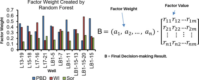
Figure 5 depicts the result of factor weights (feature importance) of three factors PBD, WI, and Sor created by the machine learning RF algorithm for every single well. The factor weights illustrated in Figure 5 are created using 3 year oilfield geology and production data. The factors calculated for each month and 36 values for PBD, WI, and Sor are created based on the mentioned oilfield historical production data. Based on this monthly factor value, the decision-making by the FEM is established. The result of the FEM was used as a remark in the RF to obtain the new factor weight. Figure 6 illustrates the well selection calculation procedure for three wells using the new weighting system generated by RF. In Figure 6, first, the monthly factor values are created for 3 years using available oilfield history data. Then, the new factor weight is generated by RF. The last part is the comprehensive evaluation to establish the decision-making well selection for water shutoff. Table 2 outlines an example of the monthly calculated factor value and result established for each moth through the new factor weight created by RF for a single well (Well13-19). It seems from Table 2 that the result for 15 months out of 26 months historical production data are confirmed as not selected for water shutoff. Therefore, the Well13-19 was not considered for water plugging in this method.
Figure 5.

Factor weight created by the RF model for every single well using 3 year historical production data.
Figure 6.

Example of the three wells’ selection procedure by the new weighting system created by the RF model.
2.3. Numerical Simulation
2.3.1. Establishment of a Geological Model and Parameter Preparation
The oil reservoir in the north Liuzan block is a key development block of Jidong Oilfield, with an exploration area of 50 km2. Since the discovery of the block in 1990, it has undergone rolling exploration and development, encryption, and improvements. The total number of wells in the simulation area is 124 with an area of 6.8 km2. According to the actual situation of the oilfield structure, the following principles should be followed when dividing the grid. The grid direction should be parallel or orthogonal to the regional boundary and well row direction as much as possible, and the grid edge should coincide with the boundary and fault as much as possible. In addition, the grid direction considers the direction of changes in reservoir properties, and the coordinate system is parallel or perpendicular to the main flow direction of the fluid in the reservoir. The grid direction and size are compatible with existing well positions and new drilling positions. The well positions are arranged in the center of the grid as much as possible, and there is only one well in a grid. Under the premise considering the abovementioned dividing principle and calculation speed, the grid is divided. The steps in the x and y directions in the plane are both 100 m. In the vertical direction, 30 small layers are divided according to the principle that the permeability difference between layers does not exceed 3. The microstructure map of the small and sand bodies of the rhythm sections in the north Liuzan block is used to control the tectonic fluctuations of the area. The Liuzan block is divided into 30 × 60 × 30 = 54,000 grids.
2.3.2. The Establishment of the Initial Static Parameter
The establishment of the initial static parameter field involves defining the spatial position of the grid used in the reservoir simulation, reservoir properties (porosity, permeability, effective thickness, or net-to-gross ratio), fluid distribution (water cut and oil saturation), temperature and pressure systems (temperature and pressure), rock and fluid compressibility, volume coefficient and viscosity, and relative permeability. Combining the composition characteristics of the CMG simulation module and the parameter definition process, the parameter definition is divided into four categories of parameters: the geological model, fluid model, fluid physical and petrophysical properties, and the field initial parameter defined one by one.
2.3.3. Reservoir Production Dynamic Parameters
Dynamic data refer to all time-related data, including well completion and workover data, production data, and pressure data. Completion data mainly include perforation, reperforation, horizon, well diameter, and the skin coefficient. The production data mainly include average monthly oil production and average monthly water production. The pressure data mainly include bottom hole pressure, shut-in static pressure, and formation pressure. There are 124 wells in the block, and the production time ranges from January 1990 to January 2040. One month is the time step, with a total of 600 time steps.
2.3.4. Production History Matching
2.3.4.1. Reserve Fitting
Based on the grid system division, the parameter interpolation operation is performed to obtain the data field of each parameter, where the balance of gravity and capillary pressure initializes the system, and the geological reserves of crude oil are compared and tested. In order to verify the geological reserves of each layer, the total geological reserves of the digital model area and the geological reserves of each district are calculated.
The main oil-producing sub-layers in the north Liuzan block are the IV1 oil group and the IV2 oil group. The relative error of the reserve fitting in the entire area is −0.52%, and the fitting accuracy is high. As shown in Table 3, the error of the single-layer reserves’ fitting is also less than 3%, which meets the accuracy requirements.
Table 3. Reserve Calculation.
| oil group | geological reserves, ×104 t | simulation calculation of reserves, ×104 t | error % |
|---|---|---|---|
| IV1 | 79.96 | 77.86 | –2.63 |
| IV2 | 92.58 | 93.79 | 1.31 |
| total | 172.54 | 171.65 | –0.52 |
2.3.4.2. Production History Matching
The actual cumulative oil production in the entire region is 88.1 × 10⁴ t, the cumulative water production is 315 × 104 t, the calculated values of the model are 97.3 × 10⁴ t and 331 × 104 t, and the relative errors are 9 and 5%, respectively. The research block contains a total of 124 wells, of which about 50 wells have been in production or water injection over the past 5 years. According to the production data obtained in the past 3 years, we have performed the fitting of production and water cut for the measure well and its surrounding wells.
-
(1)
Fluid production fitting
After adjusting the relative permeability and production measures of the numerical simulation model in the north Liuzan block, the fluid production of oil wells in the LB1-6 well group fitted over the past 3 years is shown in Figure 7. As shown in Figure 7, the average daily fluid production of well LB1-15 over the past 3 years is about 60 m3, and the simulated average fluid production is about 57 m3. The errors of the two are within the allowable range.
-
(2)
Water-bearing fitting
After adjusting the relative permeability and production measures of the numerical simulation model in the north Liuzan block, we fitted the water cut of the oil wells in the LB1-6 well group in the 3 year production data. As shown in Figure 8, the average water cut of well LB1-15 is about 86%, and the simulated average water cut is about 90%. The errors of the two are within the allowable range.
Figure 7.

LB1-15 oil well fluid production fitting.
Figure 8.

LB1-15 oil well water cut fitting.
2.3.5. Influence of Well Plugging
The gel used in this numerical simulation study is a polymer system composed of polyacrylamide with phenol and formaldehyde X-linkers.41−44 Initially, the simulation is applied to the wells judged to be blocked by the FEM. Then, the recovery factor of the selected wells by the new factor weight created by the RF model is compared with the FEM result and its effect on production is analyzed.
In the simulation model, the production wells selected for plugging are converted to gel injection wells with the gel injected for 3 days. The wells are kept shut-in for another 2 days for the polymer and X-linker to process, after which the production wells are opened to resume production. In the simulation, 16 wells selected by the FEM and 8 wells selected by the new factor weight created by the RF model have been plugged by in-suite gel. The components of injection fluid mole fractions are as follows: water is 0.999731, the polymer is 5.43 × 10⁻⁶, and the X-linker is 0.000264; they were injected in the production wells. The injection surface water rate has been considered 50 m3/day.
3. Results and Discussion
3.1. Fuzzy Evaluation Method (FEM) Result
Based on the FEM, the comprehensive decision-making average value calculated and shown in Figure 9 is B̅= 1.025. If the comprehensive evaluation value (B) is bigger than the average value (B̅), the well will not need to consider for water shutoff. From the result, it is observed that the wells with the higher PBD value are not considered for the water shutoff. The result in Figure 9 illustrates that the PBD value has direct influence to the well selection process. Figure 9 shows that 16 wells out of 21 candidate wells have been selected for water shutoff, while wells L17-21, LB1-5, LB1-11, LB1-17, and LB1-29 have not been selected for well-plugging water shutoff.
Figure 9.

Well selection results for water shutoff by the FEM.
3.2. Random Forest (RF) Result
Table 4 reports the final well selection results using the new factor weight created by the RF algorithm. It can be observed that from 21 candidate wells, eight wells are selected for water plugging and further water shutoff treatments.
Table 4. Well Selection for Water Shutoff Using the New Factor Weight Created by the RF Model Using 3 Year Production History Data.
| no | well-ID | well selection results using the new factor weight created by RF |
|---|---|---|
| 1 | L13-19 | not selected |
| 2 | L15-18 | not selected |
| 3 | L17-16 | not selected |
| 4 | L17-21 | selected |
| 5 | LB1-11 | selected |
| 6 | LB1-15-13 | not selected |
| 7 | LB1-15 | not selected |
| 8 | LB1-17 | selected |
| 9 | LB1-19 | selected |
| 10 | LB1-21 | selected |
| 11 | LB1-23 | not selected |
| 12 | LB1-25 | selected |
| 13 | LB1-26 | selected |
| 14 | LB1-29 | not selected |
| 15 | LB1-31 | not selected |
| 16 | LB1-35 | selected |
| 17 | LB1-7 | not selected |
| 18 | LB2-15-21 | not selected |
| 19 | LBJ1-24 | not selected |
| 20 | LB1-5 | not selected |
| 21 | LB1-15-13 | not selected |
3.3. Numerical Simulation Result
To evaluate the efficiency of well plugging of the wells selected by both models, the length of the effective period, water reduction and oil increment in the effective period, average water reduction per day and average oil increment per day in the effective period, and cumulative oil production at 5 years after gel injection have been compared. The effective period refers to the time from the reopening of the producer to the time when water cut rebounds to the point when the producer was shut in. The effective period can be seen as the length of the days that gel treatment has an influence on water reduction.
After 5 days of the gel injection and waiting time for the plugging process, the producer wells are reopened. The producer wells take a longer time to reach water cut as the value of the water cut increases. However, in terms of reducing production water during the effective period, the wells selected by the new factor weight created by the RF model, water cut has a better effect. Considering increasing the oil production during the effective period, the wells selected by the FEM, water cut can achieve the best result. The well-plugging result for the wells selected by the FEM, water cut is very low compared to the new factor weight created by the RF model, and the effective period can be 1800 days. Figure 10 compares the two methods FEM and new factor weight created by RF in terms of water cut, the cumulative oil production rate, and daily oil production rate. Regarding average values in the effective period of water reduction and oil increment per day, the best results are from the new factor weight created by the RF model well selection. The average values belong to the efficiency of the effects the gel injection makes. The case with wells selected by the new factor weight created by the RF model has better efficiency in reducing water and increasing oil. Table 5 outlines the cumulative oil production rate, daily oil rate average production rate, and water cut average of the base model, FEM, and using new factor weight created by the RF model.
Figure 10.

Influence of gel plugging on (a) cumulative oil production, (b) oil rate daily production, and (c) water cut of the reservoir for wells selected by the FEM, new factor weight created by RF, and base models.
Table 5. Influence of Gel Plugging Results of the Two Models and a Comparison with the Base Model.
| model | cumulative oil production (m3) 1/1/2020–1/1/2025 | oil rate daily (m3/day) production average 1/1/2020–1/1/2025 | water cut SC-% average 1/1/2020–1/1/2025 |
|---|---|---|---|
| base model | 316,763 | 173.37 | 69.543 |
| wells selected by the FEM | 319,292 | 174.75 | 69.345 |
| wells selected by using the new factor weight | 320,518 | 175.42 | 69.042 |
The well plugging influences in terms of cumulative oil production rate, daily oil production rate, and water cut of well LB1-7 selected by the FEM plus well LB1-17 selected to be plugged using the new factor weight created by RF are illustrated in Figures 11 and 12, respectively. Figure 11 displays the cumulative oil production rate, daily oil production rate, and water cut rate of well LB1-7 for the base model and FEM. Comparing the graphs illustrated in Figure 11, it can be observed that the production rate has grown compared to the base model, while water cut has diminished. This is one of the best results among the 16 wells selected by the FEM. However, the influence of the well plugging by gel has been very low in most of the wells selected by the mentioned method. Figure 12 illustrates the cumulative oil production rate, daily oil production rate, and water cut rate of well LB1-17 for the base model and using the new factor weight created by the RF model. The comparison of the graphs illustrated in Figure 12 indicates that there is a very small change in terms of the production rate and water cut compared to the base model.
Figure 11.

Influence of gel plugging on (a) cumulative oil production, (b) oil rate daily production, and (c) water cut of the well LB1-7 selected based on the FEM.
Figure 12.

Influence of gel plugging on (a) cumulative oil production, (b) oil rate daily production, and (c) water cut of the well LB1-17 selected based on the new factor weight created by the RF algorithm.
Various methods may be used to calculate the factor weight in the FEM. Some of these include the entropy method, the analytic hierarchy process, the criterion importance method, and the inter-criteria correlation.44−53 In this paper, the weight of entropy is compared with the result derived from the FEM and RF method. In 2009, Weiguo et al.24 introduced the entropy method to determine the factor weight. It does so by estimating the amount of information that is available in a given system.
The weight calculation by the entropy method is compared to the procedure presented in this paper. The calculation of the weight by the entropy method is performed on the same set of data as the FEM, and the PBD, WI, and Sor values are 0.66, 0.23, and 0.11, respectively. The well selection result obtained by the entropy method is equal to the FEM; however, it has a significant difference from the RF method. In the RF method, it is very simple to expand the data and calculate the factor weight using production history. Unfortunately, the traditional factor weight calculation methods are still not very accurate and time-consuming. This paper proposes a new method called RF, which is more advantageous and simple to use.
4. Conclusions
In this paper, a decision-making method for water shutoff well selection is established. The main controlling factors affecting water shutoff are clarified. By combining a machine learning random forest (RF) algorithm and fuzzy evaluation method (FEM), a well selection decision-making model was established. The injection parameters for the water shutoff of a typical well group were given. After the water shutoff of the well group is implemented, the oilfield reduced water and increased oil production, while the surrounding oil wells have obvious effects. After the water shutoff of the wells selected by the FEM and using the new factor weight created by RF, the cumulative oil increases during the effective periods are 2529 m3 (0.8%) and 3755 m3 (1.2%), respectively. The major conclusion obtained from this research are as follows:
-
(1)
The machine learning RF algorithm uses the historical production data of the oilfield to calculate accurate factor weight.
-
(2)
By comparing the well selection made by the FEM and the factor weight created by RF through the numerical simulation model, it has been concluded that the creation of the new factor weight can provide a sufficient effect on the water cut and oil production rate.
-
(3)
The predictive decision-making model is suggested for water shutoff, which can be used by reservoir engineers to decide which well needs to be plugged.
-
(4)
The results of the new factor weight created by the RF method and FEM are compared with the entropy factor weight method.
Acknowledgments
The authors gratefully thank the China University of Petroleum–Beijing for providing an excellent environment for research.
The authors declare no competing financial interest.
References
- Khojastehmehr M.; Madani M.; Daryasafar A. Screening of enhanced oil recovery techniques for Iranian oil reservoirs using TOPSIS algorithm. Energy Reports. 2019, 5, 529–544. 10.1016/j.egyr.2019.04.011. [DOI] [Google Scholar]
- Höök M.; Hirsch R.; Aleklett K. Giant oil field decline rates and their influence on world oil production. Energy Policy. 2009, 37, 2262–2272. 10.1016/j.enpol.2009.02.020. [DOI] [Google Scholar]
- Höök M.; Xu T.; Xiongqi P.; Aleklett K. Development journey and outlook of Chinese giant oil fields. Pet. Explor. Dev. 2010, 37, 237–249. 10.1016/S1876-3804(10)60030-4. [DOI] [Google Scholar]
- Luo P. The method of profile control for water injection wells. Oil and Gas Well Testing 2005, 14, 42–43. [Google Scholar]; original in Chinese.
- Qiao E.; Li Y.; Liu P. Oilfield block overall profile control pressure index decision-making technology and its application. Drill Mining Technology 2000, 23, 28–31. [Google Scholar]; Original in Chinese
- Song W.; Yang C.; Han D.; Qu Z.; Wang B.; Jia W.. Alkaline-surfactant-polymer Combination Flooding for Improving Recovery of the Oil with High Acid Value. SPE-29905. 1995, International Meeting on Petroleum Engineering held in Beijing, PR China, at 14–17 November 1995.
- Grigg R.B.; Schechter D.S.. State of the Industry in CO2 Floods. SPE-38849. 1997,presented at the SPE Annual Technical Conference and Exhibition held in San Antonio, Texas, USA, 5–8 October 1997. [Google Scholar]
- Xia T.; Feng Q.; Wang S.; Zhang X.; Ma Z.. Decision-Making Technology of Well Candidates Selection in In-depth Profile Control Based on Projection Pursuit Clustering Model. Proceedings of the International Field Exploration and Development Conference 2019. IFEDC. 2020, Springer Series in Geomechanics and Geoengineering. Springer, Singapore. [Google Scholar]
- Su Y.; Li Y.; Wang L.; He Y.. Experimental and pilot tests of deep profile control by injecting small slug-size nano-microsphere in offshore oil fields. Offshore Technology Conference. 2019. [Google Scholar]
- Qiu Y.; Wei M.; Bai B.; Mao C. Data analysis and application guidelines for the microgel field applications. Fuel 2017, 210, 557–568. 10.1016/j.fuel.2017.08.094. [DOI] [Google Scholar]
- Qiu Y.; Wei M.; Bai B. Descriptive statistical analysis for the PPG field applications in China: screening guidelines, design considerations, and performances. J. Pet. Sci. Eng. 2017, 153, 1–11. 10.1016/j.petrol.2017.03.030. [DOI] [Google Scholar]
- Feng Q.; Chen Y.; Jiang H.; Wang S. Application of fuzzy mathematics to block-wide injection profile control. Pet. Explor. Dev. 1998, 25, 76–79. [Google Scholar]
- Liu Y.Z.; Bai B.. Optimization Design for Conformance Control Based on Profile Modification Treatments of Multiple Injectors in a Reservoir. SPE-64731. 2000, presented at the SPE International Oil and Gas Conference and Exhibition in China held in Beijing, China, 7–10 November 2000.
- Liu Y. Z.; Bai B.; Li Y. X.; Coste J. P.; Guo X. H.. Optimization Design for Conformance Control Based on Profile Modification Treatments of Multiple Injectors in a Reservoir. SPE-64731-MS. 2000, Presented at the International Oil and Gas Conference and Exhibition in China, Beijing, China, November 2000.
- Jiang H. Q.; Wang S. L.; Zhang Y. Pre-Warning and Decision Making of Water Breakthrough for Higher Water-Cut Oil Field. Adv. Mater. Res. 2011, 347–353, 688–693. [Google Scholar]
- Li X. Application of Fuzzy Mathematics Evaluation Method in Prediction of Comprehensive Efficiency of Low-Efficiency Oil Wells. IOP Conference Series Earth and Environmental Science 2019, 384, 012012 10.1088/1755-1315/384/1/012012. [DOI] [Google Scholar]
- Zhang X.; Li Q.; Li X. The application of fuzzy mathematics in the optimization of oilfield development scheme. Northwest Geol. 2002, 1, 76–80. [Google Scholar]
- Tang H.; Huang B.; Li D. Fuzzy comprehensive evaluation method to determine the potential of reservoir water flooding development. Pet. Explor. Dev. 2002, 2, 97–99. [Google Scholar]
- Wang Y. Application of PI decision-making technology in Zhongyuan oil field. Pet. Explor. Dev. 1999, 26, 81–83. [Google Scholar]
- Li Y. K. Pressure Index Decision Technology for Integrated Profile Control in a Block. J. Univ. Pet. China. 1997, 21, 39–42. [Google Scholar]
- Qin G.; Pan P.; Tao H. The analysis and application of PI decision making technology. Neimenggu Shiyou Huagong. 2005, 8, 120–123. [Google Scholar]; (In Chinese)
- Yu Z. PI decision technology in Gudong Oilfield application. Xibu Tankuang Gongcheng. 2005, 8, 53–54. [Google Scholar]; (In Chinese)
- Liu Y.; Bai B.; Wang Y. Applied Technologies and Prospects of Conformance Control Treatments in China. Oil & Gas Science and Technology - Revued’IFP Energies nouvelles, Institut Français du Pétrole. 2010, 65, 859–878. 10.2516/ogst/2009057. [DOI] [Google Scholar]
- Weiguo Z.; Gichong T. The Application of Entropy Method and AHP in Weight Determining. Computer Program Skills and Maintenance. 2009, 22, 19–20. [Google Scholar]
- Krasnov F.; Glavnov N.; Sitnikov A. Application of Multidimensional Interpolation and Random Forest Regression to Enhanced Oil Recovery Modeling. ACM Comput. Entertain. 2017, 9, 9. [Google Scholar]
- Donges N.A complete guide to the random forest algorithm. https://builtin.com/data-science/random-forest-algorithm. June, 2019, update, July 2021.
- Walt S. V. D.; Colbert S. C.; Varoquaux G. The NumPy Array: A Structure for Efficient Numerical Computation. Comput. Sci. Eng. 2011, 13, 22–30. 10.1109/MCSE.2011.37. [DOI] [Google Scholar]
- McKinney W.Data structures for statistical computing in python. Proceedings of the 9th Python in Science Conference. 2010, 445. SciPy Austin, TX, 51–56, 10.25080/Majora-92bf1922-00a. [DOI] [Google Scholar]
- Jones E.; Oliphant T.; Peterson P.. SciPy. open source scientific tools for Python. 2014.
- Pedregosa F.; Varoquau G.; Gramfort A.; Michel V.; Thirion B.; Grisel O.; Blondel M.; Prettenhofer P.; Weiss R.; Dubourg V.; Vanderplas J.; Passos A.; Cournapeau D. Scikit-learn: Machine Learning in Python. Journal of Machine Learning Research. 2011, 12, 2825–2830. [Google Scholar]
- Millman K. J.; Aivazis M. Python for Scientists and Engineers. Comput. Sci. Eng. 2011, 13, 9–12. 10.1109/MCSE.2011.36. [DOI] [Google Scholar]
- Li Z. C. The PI Decision Theory Application of Multi-Round Profile Control. Appl. Mech. Mater. 2013, 295-298, 3302–3305. 10.4028/www.scientific.net/AMM.295-298.3302. [DOI] [Google Scholar]
- Horner D. R.Pressure Buildup in Wells, Proc., Third World Pet. Congo. 1951, Sect. II, 503. [Google Scholar]
- Perrine R. L. Analysis of pressure buildup curves. drilling and production practice. API 1956, 482–509. [Google Scholar]
- Breiman L. Random Forests. Machine Learning. 2001, 45, 5–32. 10.1023/A:1010933404324. [DOI] [Google Scholar]
- Catani F.; Lagomarsino D.; Segoni S.; Tofani V. Landslide susceptibility estimation by random forests technique: sensitivity and scaling issues. Nat Hazards Earth Syst Sci. 2013, 13, 2815–2831. 10.5194/nhess-13-2815-2013. [DOI] [Google Scholar]
- Liaw A.; Wiener M. Classification and regression by random forest. R News. 2002, 2, 18–22. [Google Scholar]
- Naghibi S. A.; Ahmadi K.; Daneshi A. Application of Support Vector Machine, Random Forest, and Genetic Algorithm Optimized Random Forest Models in Groundwater Potential Mapping. Water Resour. Manage. Ser. 2017, 31, 2761–2775. 10.1007/s11269-017-1660-3. [DOI] [Google Scholar]
- Random Forest Algorithm, Java T point. https://www.javatpoint.com/machine-learning-random-forest-algorithm, this subject taken at July, 2021.
- Brownlee J.How to Calculate Feature Importance With Python. Machine learning mastery. 2020https://machinelearningmastery.com/calculate-feature-importance-with-python/. [Google Scholar]
- Zhu D.; Bai B.; Hou J. Polymer Gel Systems for Water Management in High-Temperature Petroleum Reservoirs: A Chemical Review. Energy Fuels 2017, 31, 13063–13087. 10.1021/acs.energyfuels.7b02897. [DOI] [Google Scholar]
- Zhu D.; Hou J.; Meng X.; Zheng Z.; Wei Q.; Chen Y.; Bai B. Effect of Different Phenolic Compounds on Performance of Organically Cross-Linked Terpolymer Gel Systems at Extremely High Temperatures. Energy Fuels 2017, 31, 8120–8130. 10.1021/acs.energyfuels.7b01386. [DOI] [Google Scholar]
- Wei J.; Zhou X.; Zhang D.; Li J. Laboratory Experimental Optimization of Gel Flooding Parameters to Enhance Oil Recovery during Field Applications. ACS Omega 2021, 6, 14968–14976. 10.1021/acsomega.1c01004. [DOI] [PMC free article] [PubMed] [Google Scholar]
- Bai B.; Zhou J.; Yin M. A comprehensive review of polyacrylamide polymer gels for conformance control. Pet. Explor. Dev. 2015, 42, 525–532. 10.1016/S1876-3804(15)30045-8. [DOI] [Google Scholar]
- Liu L.; Zhou J.; An X.; Zhang Y.; Yang L. Using fuzzy theory and information entropy for water quality assessment in Three Gorges region, China. Expert System with Application. 2010, 37, 2517–2521. 10.1016/j.eswa.2009.08.004. [DOI] [Google Scholar]
- Amiri V.; Rezaei M.; Sohrabi N. Groundwater quality assessment using entropy weighted water quality index (EWQI) in Lenjanat. Iran. Environ. Earth Sci. 2014, 72, 3479–3490. 10.1007/s12665-014-3255-0. [DOI] [Google Scholar]
- Zhang P.; Feng G. Application of fuzzy comprehensive evaluation to evaluate the efect of water fooding development. J. Pet. Explor. Prod. Technol. 2018, 8, 1455–1463. 10.1007/s13202-018-0430-y. [DOI] [Google Scholar]
- Hsu L. Using a Decision-Making Process to Evaluate Efficiency and Operating Performance for Listed Semiconductor Companies. Technological and Economic Development of Economy. 2017, 21, 301–331. [Google Scholar]
- Zhang H. Application on the Entropy Method for Determination of Weight of Evaluating Index in Fuzzy Mathematics for Wine Quality Assessment. Adv. J. Food Sci. Technol. 2015, 7, 195–198. 10.19026/ajfst.7.1293. [DOI] [Google Scholar]
- Şahin M. A comprehensive analysis of weighting and multicriteria methods in the context of sustainable energy. Int. J. Environ. Sci. Technol. 2021, 18, 1591–1616. 10.1007/s13762-020-02922-7. [DOI] [PMC free article] [PubMed] [Google Scholar]
- Menglin X.; Deshen Z. Application of Entropy-Weight Hierarchy Analysis on Study of Height Prediction of Water Conducted Zone. Adv. Mater. Res. 2013, 742, 497–500. [Google Scholar]
- Zhu Y.; Tian D.; Yan F. Effectiveness of Entropy Weight Method in Decision-Making. Math. Probl. Eng. 2020, 3564835. 10.1155/2020/3564835. [DOI] [Google Scholar]
- Al-Aomar R. A Combined AHP-Entropy Method for Deriving Subjective and Objective Criteria Weights. International Journal of Industrial Engineering. 2010, 17, 12–24. [Google Scholar]