Principles of mathematical epidemiology and compartmental modelling application to COVID-19

Along with the start of the SARS-CoV-2 pandemic, mathematical epidemiology quickly reached a new and broader audience in early 2020 [1]. If epidemiological models were sometimes recognised as useful tools for decision support, their relevance was also challenged, notably among decision-makers, but also by health workers and the public. While their scope and their limitations must be acknowledged [2], the understanding of the modelling principles and main assumptions by non-specialists appears essential for both transdisciplinary improvement and better use of their results.

Modelling is a rational simplification of a phenomenon, a formalisation that focuses on the parts considered to be essential to generate the observed patterns. In the case of infectious diseases, the mathematical equations on which the models of their spread are based share a common backbone corresponding to transmission and recovery events, while the vast diversity of details depends on the pathogen, host population, prevention, and treatments considered [3].

The choice of the starting assumptions and the formalism will essentially depend on the initial question but might as well be oriented by the kind of data available to calibrate the parameters.

Most models designed to capture the spread of an epidemic in a given population are said compartmental. These models are related to the seminal work of Kermack and McKendrick known as the SIR model, where the population is divided into three compartments: susceptible ($S$), infected ($I$), and removed ($R$) [4]. The model follows the change in the proportion of the population belonging to each compartment through time, by reproducing numerically the course of infectious diseases epidemics: an infectious individual transmits the disease to a susceptible individual, who becomes infectious and then transmits the disease at his turn (perpetuating the epidemic), before recovering (or dying) from the disease, assuming no further contribution to the spread of the disease.

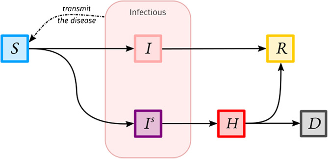
Advanced and current models are designed with a higher number of connected compartments to better reflect the clinical and epidemiological features and outcomes of the disease, as well as to match a particular question and the data on which dynamical inference can be done. For instance, one of the main questions addressed by models during the first wave of the SARS-CoV-2 epidemic in France (in March 2020) was how many people at most would be simultaneously hospitalised due to COVID-19, to prevent or at least anticipate a hospital overload. In such a case, a compartment for hospitalised infected individuals is then introduced. On a first approach, we could imagine a model with a compartment for infected individuals who will develop a mild or asymptomatic form of the disease and another compartment for infected individuals who will develop a severe form of the disease and will require a later hospitalisation before recovery or death, as represented by the illustrative model presented on Fig. 1 . This simple model can be further improved by adding new compartments and be amended on a second approach provided new knowledge or data (e.g. specifying an incubation period).

Fig. 1.

Illustrative compartmental model to estimate hospital occupancy. Susceptible individuals ($S$compartment) become infected after being in contact with infected individuals. They can develop an asymptomatic or mild version of the disease ($I$) before recovering ($R$), or they can become severely infected ($I^s$). In the latter, they will transmit the disease as the other infected individuals then end up in the hospital ($H$) before recovery or death ($D$).

There also exist different mathematical formalisms such as discrete-time modelling (see Ref. [5]), based on a system of partial differential equations (e.g. Ref. [6]) or even individual-based stochastic simulations [7], but the most common remains the use of a system of ordinary differential equations (ODE) [3], that is a set of conditions on the derivatives of unknown functions. These functions are simply the number of individuals in each compartment through time.

Instead of trying to estimate at each time step the proportion of the population in each compartment, which would be somehow very tedious, we simply estimate the number of individuals who move from one compartment to another.

Thus, we need to know only two things:

• 1the state of the epidemic at a given time $t$ ;
• 2what happens during the following small-time interval $\Delta t$.

The first step is usually straightforward since we might just consider the beginning of the epidemic where every individual but one is susceptible. The second step however represents the mathematical translation of disease dynamics. For instance, if we consider the model presented beforehand, the number of susceptible $S$ individuals at time $t+\Delta t$ is given by the number of susceptible individuals at time, minus the individuals that got infected between $t$ and $+\Delta t$. Assuming that the probability of infection is proportional to the current number of contagious individuals:

$$S\left(t+\Delta t\right)=S\left(t\right)-\beta S\left(t\right)I_{tot}\left(t\right)\Delta t$$

where $\beta$ is the transmission rate, which represents, for each susceptible individual, the probability of being infected per unit of time and per capita of currently contagious individuals in the population. Hence, we need to know the transmission rate, which is often estimated on incidence data using external statistical procedures (e.g. reproduction number estimation as in Ref. [8]). We also need to know the current total number of individuals infected ($I_{tot}\left(t\right)=I\left(t\right)+I^s\left(t\right)$), which implies the different compartments must be followed simultaneously.

This idea is generalised for each compartment: we determine at each time step the inflows and outflows related to each compartment. Within a compartment, inflows correspond to a certain number of individuals per time unit leaving other compartments, and departures are done with a constant rate – meaning at each time step a constant proportion of the individuals in the compartment leaves the compartment. Note that in the simplest models, the force of infection (the rate at which susceptible individuals become infected) is the only time-varying rate (as a function of the prevalence) and therefore captures the whole non-linearity of the dynamics. In more sophisticated models (e.g., weather effect, variant replacement, public health interventions such as transient social distancing or vaccination program, immune waning), otherwise constant rates would explicitly depend on time, therefore greatly increasing the richness of the dynamics.

As for any quantitative approach, such models rely on simplifying assumptions which constitute inherent limitations. The main ones are the lack of spatial structure (all encounters have the same probability to occur) and host heterogeneity (inter-individual differences are smoothed out). Despite their unrealistic nature, these assumptions have proved to provide robust and conservative estimates in the early stages of an epidemic [9]. On a longer timescale, however, increasing the number of compartments to introduce a form of spatial structure and/or individual heterogeneity is both common and straightforward [3]. This might be e.g., an age structure to take into account age-differentiated severity as for COVID-19 or add gender structure for modelling sexually-transmitted infections. However, adding a structure needs further knowledge (literature, expertise, and data) to be implemented.

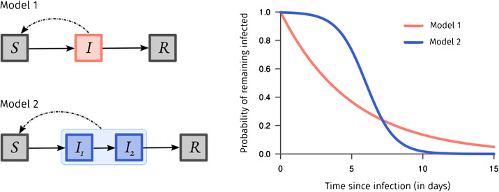
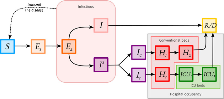
Another caveat, specific to the ODE formalism presented here, concerns the rate-based departures of the compartments. It indeed implies the time spent for an individual in a compartment does not depend on the time already spent in the compartment (which is rarely true). A workaround consists in chaining many compartments of a given clinical-epidemiological stage to shape the probability for an individual to go to the next stage according to the time already spent, as explained in Fig. 2 . For instance, Ref. [10] developed a model to estimate hospital occupancy in France in 2020. This model is shown in Fig. 3 , it is structured by the age of the individuals. The difference in the number of compartments between Fig. 1, Fig. 3 is mainly due to correcting the residency time memory problem mentioned beforehand.

Fig. 2.

The probability for a given individual of remaining in a specific compartment in a classical and simple SIR model, like the infected compartment ($I$) in Model 1 follows an exponential distribution which is memoryless – meaning the time spent in the compartment does not depend on the time already spent in the compartment, which is unrealistic. A workaround consists of chaining compartments as $I_1$ and $I_2$ in Model 2, thus creating some heterogeneity and adding memory. For instance, to specify that an individual who just entered a compartment has a very low probability to clear the disease instantly, and on the contrary if she/he spent already some significant time infected, she/he has a higher probability to clear the disease.

Fig. 3.

The model used by Ref. [10] to estimate the hospital conventional beds occupancy and ICU beds occupancy. In this model, individuals can be either susceptible ($S$), exposed ($E$), infected but not hospitalised ($I$), hospitalised in conventional beds ($H$), hospitalised in ICU ($ICU$) or removed ($R/D$).

From models, we can also retrieve the basic reproduction number, $R_0$, that is the average number of secondary infections caused by an index case [11]. This key epidemiological descriptor quantifies not only the contagiousness of the disease but also relates to the epidemic risk (what is the probability for an outbreak to occur?), the herd immunity (what is the minimum vaccine coverage to prevent any further outbreak?) threshold and the attack rate (what is the proportion of individuals eventually infected in absence of intervention?). This might be intuitively seen as

R₀ = number of contacts per day × probability of transmission per contact × infection duration (in days).

Its precise derivation however depends on the considered model. In a simple SIR model, the $I$ compartment satisfies

$$I\left(t+\Delta t\right)-I\left(t\right)=\beta \Delta tS\left(t\right)I\left(t\right)-\gamma I\left(t\right)\Delta t,$$

where $\beta$ is the transmission rate and $\gamma$ is the recovery rate. In this setting, an outbreak occurs whenever there is an initial increase of the number of infected individuals. From a mathematical point of view, this corresponds to a positive derivative of prevalence at $t=0$, $\left(I\left(\Delta t\right)-I\left(0\right)\right)/\Delta t>0$, which, using the previous equation, can be rewritten as

$$1<\frac{\beta S\left(0\right)}{\gamma }=R_{0.}$$

As immunity builds up in the population (and assuming no immune waning nor variant), the average number of secondary infections per case eventually decreases to lower values and the epidemic dynamics are then described by its real-time analog, namely the temporal reproduction number $R_t$.

One of the major criticisms against those models is that predictions would be wrong. It is worth to note such mechanistic models usually are not (and should not) aimed to predict the future, but simulate the most likely trends given a set of assumptions like a pre-established contact rate among the population. In a one-year retrospective analysis, Ref. [12] showed that such projections can help anticipate COVID-19 critical care bed occupancy for more than a month, on average. However, mechanistic models perform poorly within two weeks that follows a steep change in the transmission pattern in the absence of previous analogous period, e.g., in the case of the first implementation of a national curfew for which the efficiency is yet unknown and requires consolidated testing data to be assessed.

Given their simplifying nature and elementary mathematical formulation, compartmental models thus represent a trade-off between flexibility, robustness, and accuracy, which explain their central role in the monitoring and control of epidemics.

Competing interests

The authors declare no competing interest.

References

- 1.Adam D. Special report: the simulations driving the world’s response to COVID-19. Nature. 2020;580(7803):316–318. doi: 10.1038/d41586-020-01003-6. [DOI] [PubMed] [Google Scholar]
- 2.Siegenfeld A.F., Taleb N.N., Bar-Yam Y. Opinion: what models can and cannot tell us about COVID-19. Proc Natl Acad Sci. 2020;117(28):16092–16095. doi: 10.1073/pnas.2011542117. [DOI] [PMC free article] [PubMed] [Google Scholar]
- 3.Keeling M.J., Rohani P. Princeton University Press; 2008. Modeling infectious diseases in humans and animals. [DOI] [Google Scholar]
- 4.Kermack W.O., McKendrick A.G. A contribution to the mathematical theory of epidemics. Proc R Soc Lond Ser Contai Pap Math Phys Character. 1927;115(772):700–721. doi: 10.1098/rspa.1927.0118. [DOI] [Google Scholar]
- 5.Sofonea M.T., Reyné B., Elie B., Djidjou-Demasse R., Selinger C., Michalakis Y., et al. Memory is key in capturing COVID-19 epidemiological dynamics. Epidemics. 2021;35 doi: 10.1016/j.epidem.2021.100459. [DOI] [PMC free article] [PubMed] [Google Scholar]
- 6.Richard Q., Alizon S., Choisy M., Sofonea M.T., Djidjou-Demasse R. Age-structured non-pharmaceutical interventions for optimal control of COVID-19 epidemic. PLoS Comput Biol. 2021;17(3) doi: 10.1371/journal.pcbi.1008776. [DOI] [PMC free article] [PubMed] [Google Scholar]
- 7.Thomine O., Alizon A., Boennec C., Barthelemy M., Sofonea M.T. Emerging dynamics from high-resolution spatial numerical epidemics. eLife. 2021;10 doi: 10.7554/eLife.71417. [DOI] [PMC free article] [PubMed] [Google Scholar]
- 8.Thompson R.N., Stockwin J.E., van Gaalen R.D., Polonsky J.A., Kamvar Z.N., Dermarsh P.A., et al. Improved inference of time-varying reproduction numbers during infectious disease outbreaks. Epidemics. 2019;29 doi: 10.1016/j.epidem.2019.100356. [DOI] [PMC free article] [PubMed] [Google Scholar]
- 9.Trapman P., Ball F., Dhersin J.S., Tran V.C., Wallinga J., Britton T. Inferring R0 in emerging epidemics—the effect of common population structure is smal. J R Soc Interface. 2016;13(121) doi: 10.1098/rsif.2016.0288. [DOI] [PMC free article] [PubMed] [Google Scholar]
- 10.Salje H., Tran Kiem C., Lefrancq N., Courtejoie N., Bosetti P., Paireau J., et al. Estimating the burden of SARS-CoV-2 in France. Science. 2020 doi: 10.1126/science.abc3517. [DOI] [PMC free article] [PubMed] [Google Scholar]
- 11.Anderson R.M., May R.M. Oxford university press; 1992. Infectious diseases of humans: dynamics and control. [Google Scholar]
- 12.Sofonea M.T., Alizon S. Anticipating COVID-19 intensive care unit capacity strain: a look back at epidemiological projections in France. Anaesth Crit Care Pain Med. 2021;40(4) doi: 10.1016/j.accpm.2021.100943. [DOI] [PMC free article] [PubMed] [Google Scholar]