

Abstract
Structural magnetic resonance imaging (sMRI) can capture the spatial patterns of brain atrophy in Alzheimer's disease (AD) and incipient dementia. Recently, many sMRI‐based deep learning methods have been developed for AD diagnosis. Some of these methods utilize neural networks to extract high‐level representations on the basis of handcrafted features, while others attempt to learn useful features from brain regions proposed by a separate module. However, these methods require considerable manual engineering. Their stepwise training procedures would introduce cascading errors. Here, we propose the parallel attention‐augmented bilinear network, a novel deep learning framework for AD diagnosis. Based on a 3D convolutional neural network, the framework directly learns both global and local features from sMRI scans without any prior knowledge. The framework is lightweight and suitable for end‐to‐end training. We evaluate the framework on two public datasets (ADNI‐1 and ADNI‐2) containing 1,340 subjects. On both the AD classification and mild cognitive impairment conversion prediction tasks, our framework achieves competitive results. Furthermore, we generate heat maps that highlight discriminative areas for visual interpretation. Experiments demonstrate the effectiveness of the proposed framework when medical priors are unavailable or the computing resources are limited. The proposed framework is general for 3D medical image analysis with both efficiency and interpretability.
Keywords: Alzheimer's disease, convolutional neural network, early diagnosis, structural MRI, visual attention
A lightweight and effective neural network for early Alzheimer's disease (AD) diagnosis. An integrated framework of feature extraction, classification, and localization. Use an asymmetrically parallel structure to extract better representations. Process whole‐brain structural MRI scans without the need of any prior knowledge.
1. INTRODUCTION
Alzheimer's disease (AD), the most common form of dementia, affects many millions of people worldwide (Livingston et al., 2017). Since there is currently no cure for AD and prompt treatment might delay disease progression (Livingston et al., 2017; Weimer & Sager, 2009), early diagnosis is of great importance. Brain atrophy is an important biomarker of both established AD and mild cognitive impairment (MCI; Jack et al., 2010; Vemuri et al., 2009), which is known as the transitional stage between normal cognition and dementia. Structural magnetic resonance imaging (sMRI) is able to capture the brain changes before the onset of dementia (Ewers, Sperling, Klunk, Weiner, & Hampel, 2011; Jack et al., 1997). As a result, many sMRI‐based computer‐aided diagnosis (CAD) algorithms have been developed for diagnosis of AD and prediction of MCI‐to‐AD conversion (Bron et al., 2015; Eskildsen et al., 2013; Khvostikov, Aderghal, Benois‐Pineau, Krylov, & Catheline, 2018; Korolev, Safiullin, Belyaev, & Dodonova, 2017; Lian, Liu, Zhang, & Shen, 2018; Lin et al., 2018; Liu, Zhang, Adeli, & Shen, 2018; Liu, Zhang, & Shen, 2016; Liu, Zhang, Yap, & Shen, 2017; Moradi et al., 2015; Rathore, Habes, Iftikhar, Shacklett, & Davatzikos, 2017; Suk et al., 2014; Tong et al., 2017; Vieira, Pinaya, & Mechelli, 2017; Zhang, Gao, Gao, Munsell, & Shen, 2016).
Existing CAD methods can be categorized into conventional learning‐based methods and deep learning‐based methods. Conventional learning‐based methods have two independent steps, handcrafted feature extraction and classifier construction (Rathore et al., 2017). Davatzikos, Bhatt, Shaw, Batmanghelich, and Trojanowski (2011) trained a support vector machine (SVM) classifier with sMRI‐based biomarkers and cerebrospinal fluid biomarkers and used it to predict which MCI patients would progress to AD. Eskildsen et al. (2013) measured cortical thickness in selected regions of interest and used the measurements to train a linear discriminant analysis (LDA) classifier for AD prediction. The feature design of conventional learning‐based methods relies on considerable and costly domain expertise. Also, separating feature design from classifier construction could cause cascading errors in the model, since the handcrafted features may not optimally represent the data.
Due to its strength in automatically extracting complex patterns, deep learning has now been employed to solve many problems in computer vision, natural language processing (LeCun, Bengio, & Hinton, 2015), and neuroimaging (Vieira et al., 2017; Zaharchuk, Gong, Wintermark, Rubin, & Langlotz, 2018). Among the neuroimaging studies, Ding et al. (2019) utilized a pre‐trained convolutional neural network (CNN) for AD diagnosis; Spasov et al. (2019) developed a CNN that learned from sMRI, demographic, neuropsychological, and genetic data for predicting MCI to AD conversion. Suk et al. (2017) first trained multiple sparse regression models with manually engineered features and then built a deep network on the basis of the regression responses and clinical scores for diagnosis.
Although existing deep learning‐based CAD methods have produced impressive results, they may still encounter some inherent limitations: (a) the risk of overfitting, (b) the difficulty in capturing discriminative patterns, and (c) the requirement for extra annotation or prior knowledge. By simply stacking neural layers, CNNs could capture representative features in a large receptive field (Luo, Li, Urtasun, & Zemel, 2018). Meanwhile, the CNNs are exposed to increased risks of overfitting as more parameters are employed. Considering the relatively small sample sizes of most neuroimaging studies, the deep learning‐based CAD models are easily troubled with overfitting issue, which leads to inferior test results. Furthermore, early diagnosis is challenging, because the spatial patterns of brain atrophy in MCI and AD are subtle and diffuse (Driscoll et al., 2009). Existing CAD methods require extra guidance to better identify the differences between different clinical groups. For example, some methods model patterns of spatial atrophy conditioned on detected landmarks (Liu et al., 2018) or predefined anatomical landmarks (Lian et al., 2018). These methods require an extra landmark detection module or a location proposal module, which was designed in an ad‐hoc manner and cannot be jointly optimized with the network, thus constraining their applications.
To solve the above problems, we propose a deep learning framework for sMRI‐based AD diagnosis. The framework accepts 3D sMRI scans as input and outputs diagnostic labels. First, we use a lightweight 3D convolutional network as the primitive feature extractor. To tackle the trade‐off between better representation learning and increased risk of overfitting, we devise a parallel attention‐augmented bilinear network (pABN), which extract fine‐grained representations with only a small parameter overhead. Specifically, the parallel attention‐augmented blocks model long‐range interdependencies and asymmetrically project the learned features to lower dimensions. Finally, the compressed features of the parallel branches are combined using bilinear pooling to model localized feature interactions. A schematic of the proposed framework is shown in Figure 1. In the experiments, we evaluate our framework on two independent datasets from Alzheimer's Disease Neuroimaging Initiative (ADNI; Jack Jr. et al., 2008) for AD classification and MCI conversion prediction.
FIGURE 1.
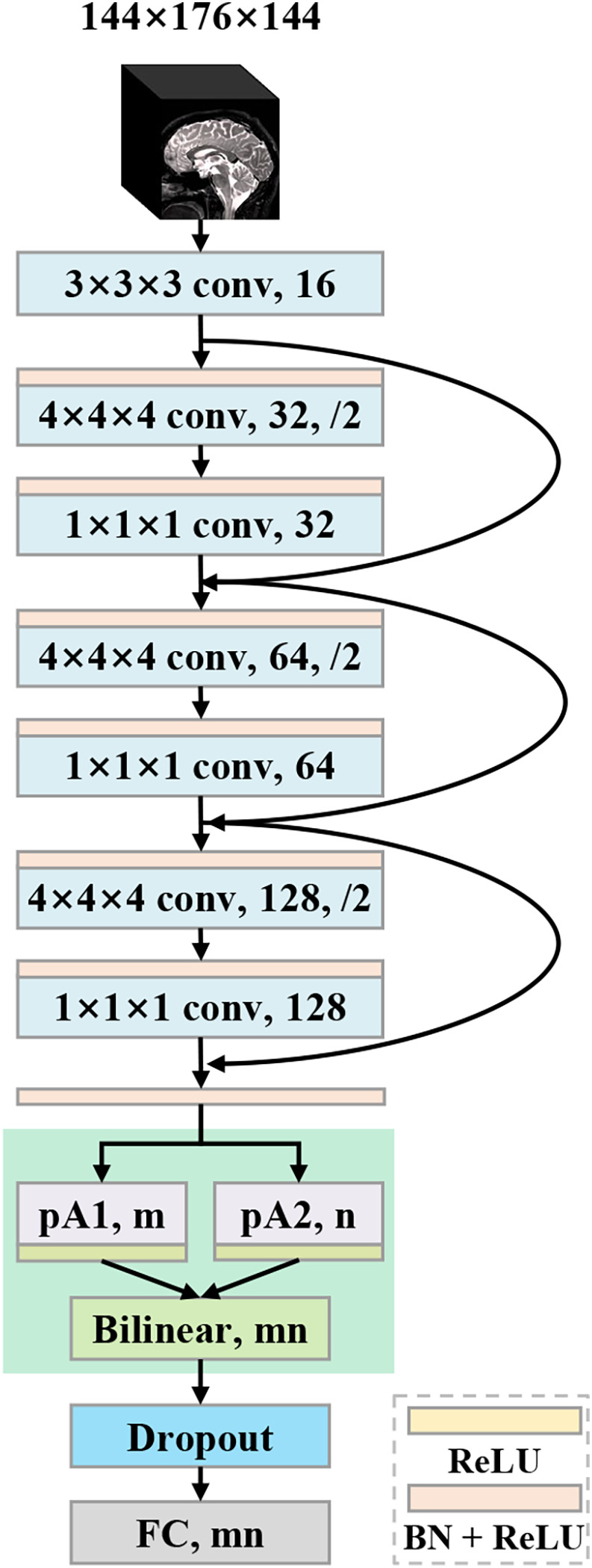
Architecture of the proposed parallel attention‐augmented bilinear network (pABN). “pA” refers to the parallel attention‐augmented blocks
The main contributions are summarized as follows:
We devise a lightweight and effective neural network for AD diagnosis and MCI conversion prediction. The network achieves competitive results with a small parameter overhead.
Unlike the previous works that require either feature extraction or discriminative region proposals before the construction of the main network, our proposed framework is an integration of automatic feature extraction, classification, and discriminative localization.
The proposed framework employs an asymmetrically parallel structure to extract better representations from whole‐brain structural MRI scans, and does not need any prior knowledge for feature learning.
2. METHOD
We next introduce the proposed pABN. First, we introduce the whole network framework and the role of each component. Then, we detail the training procedure and implementation.
2.1. pABN
Taking a 3D brain image as input, a backbone network first extracts primitive features, which are then passed to parallel attention‐augmented blocks for extracting long‐range interactions. To further refine local features, the learned feature maps are fused with bilinear pooling. Finally, a fully connected layer with two output units is used as the classifier. The network architecture (Figure 1) is described in detail below.
2.1.1. Backbone network
The backbone network is based on ResNet (He, Zhang, Ren, & Sun, 2016a) using residual units proposed in (He, Zhang, Ren, & Sun, 2016b). The network architecture consists of a root convolutional layer and three residual units. The root convolutional layer accepts the 3D images, with 3D kernel of size 3 × 3 × 3 and 16 output channels. The next three residual units have the same structure except for the output channels. To cover regions of interest with a sufficiently large receptive field, we choose to use a large kernel size for convolutions. In addition, we use strided convolutions to down‐sample the features. Feature down‐sampling is achieved via strided convolutions. No average‐pooling or max‐pooling layer is used. Specifically, each residual unit has two convolutional layers: the first layer has kernels of size 4 × 4 × 4 with stride 2; the next layer has kernels of size 1 × 1 × 1 with stride 1. The number of output channels is doubled for the first layer while unchanged for the second layer. The layer with kernel size 4 × 4 × 4 symmetrically applies zero paddings to ensure that the output feature map is exactly half the size of the input feature map. Before each convolutional layer, a batchnorm (BN) layer (Ioffe & Szegedy, 2015) and a rectified linear unit (ReLU) (Glorot, Bordes, & Bengio, 2015) are cascaded. After three residual units, the feature map is down‐sampled eight times to 18 × 22 × 18. Then, another combination of BN and ReLU is inserted before the next parallel attention‐augmented blocks.
2.1.2. Parallel attention‐augmented blocks
Most existing convolutional neural networks are constructed by serially stacking convolutional layers. Although a network's capacity generally increases as the number of layers increases, the network also tends to overfit a small dataset because of huge amount of parameters. In our framework, we devise the parallel attention‐augmented blocks (pA‐blocks) to solve this problem. Our pA‐blocks are based on the double attention block (A2‐block) proposed by Chen, Kalantidis, Li, Yan, and Feng (2018), which aims to effectively capture the global information and distribute it to every location in a two‐step attention manner. In this way, each location in the feature map receives customized global information as complements, thereby enabling the network to learn more complex relationships. Different from the original A2‐block, we modify it to facilitate a parallel structure with augmented representation spaces and less trainable parameters.
The structure of the modified A2‐block is shown in Figure 2. denotes the input feature for the 3D convolutional layer, where denotes the number of channels, and are the spatial dimensions. The block contains three 3D convolutional layers with 1 × 1 × 1 kernel and m output channels. After necessary reshaping and transposing operations, we have feature maps generated by convolutional layers: where each is a dhw‐dimensional row vector, and In the first attention step, global representations are gathered effectively by second‐order attention pooling. is the output of the first attention step. In the second attention step, global features are adaptively distributed to each spatial location. is the output of the second attention step. Specifically:
| (1) |
| (2) |
In the original implementation (Chen et al., 2018), is fed into another convolutional layer to expand the number of channels and then encoded back to input via element‐wise addition. By contrast, we (Figure 2) remove the extra convolutional layer that projects the representation back into the input space. The final output of the A2‐block is generated by encoding back to via element‐wise addition. This modification results in fewer parameters and less complexity of the block and further reduces the number of parameters in the last classifier. Given the numbers of output channels of the block's three convolutional layers (i.e., m) and the backbone network (i.e., 128), the number of parameters within the modified A2‐block is calculated by 128 × 3 × m.
FIGURE 2.
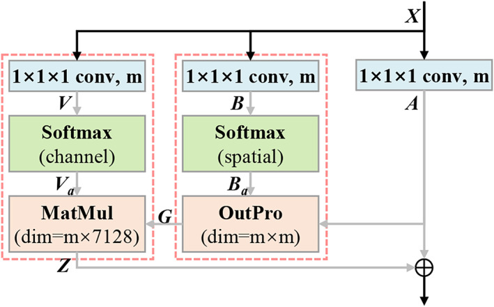
A flowchart showing the modified double attention block used in the present study. Specifically, “m” represents number of channels of the convolutional layer, and “7,128” represents the product of the spatial dims of the feature map (i.e., dhw = 18 × 22 × 18 = 7,128); “MatMul” represents matrix multiplication; “OutPro” represents outer product
On top of the backbone network, we use two modified A2‐blocks in a parallel structure (Figure 1) to construct the pA‐blocks. The pA‐blocks are initialized independently and trained jointly. We use n to represent the number of output channels of the second block. The network's capacity is increased by pA‐blocks attending to different representation subspaces. Then, we investigate the network's ability to capture various spatial interactions by setting pA‐blocks in a symmetric structure with the same numbers of output channels (i.e., m = n) or in an asymmetric structure with different numbers of output channels (i.e., m ≠ n). The asymmetrically parallel structure provides a unique solution space and is expected to further enhance the network's representation power.
2.1.3. Bilinear pooling
Global average pooling is an aggressive information gathering approach, which fails to capture complex interactions, especially when the network is shallow. We use bilinear pooling to fuse the features learned by the previous pA‐blocks. Bilinear pooling can capture pairwise correlations between feature channels and model part‐feature interactions (Lin, RoyChowdhury, & Maji, 2015). In brief, we use outer product to multiply the feature maps of the pA‐blocks at each location and pool across locations. Note that no priors of discriminative locations are needed when using the bilinear model.
Specifically, and are the two activated feature maps, where are the output channels. Bilinear combinations of features across all locations are then aggregated using sum pooling to obtain a global image representation :
| (3) |
The bilinear feature is an orderless representation since the feature locations are ignored. Following Lin et al. (2015), the feature is passed through a signed square root followed by normalization. The normalized bilinear feature is then flattened into a vector, followed by a dropout layer (Srivastava, Hinton, Krizhevsky, Sutskever, & Salakhutdinov, 2014). Finally, a fully connected layer with two output units is applied as a linear classifier.
2.2. Implementation
We next introduce the data augmentation procedure, training objective, transfer learning, and visual interpretation methods.
2.2.1. Data augmentation
While random cropping is routinely used for data augmentation in deep learning, it is wasteful to shift the brains after nonlinear registration. In addition, most data augmentation methods significantly increase the computational cost, which is even worse when dealing with 3D data. We instead use mixup (Zhang, Cisse, Dauphin, & Lopez‐Paz, 2017), a simple learning principle, to train the deep learning model on convex combinations of pairs of examples and their labels. Mixup regularizes the neural network to favor simple linear behavior between training examples. This linear behavior increases the generalization of the model for predicting outside the training examples. Formally:
| (4) |
| (5) |
where for and and are two data‐target vectors drawn randomly from the training data. Specifically, and represent the one‐hot label encodings. After augmentation, are used for training. In our implementation, mixup is applied to each mini‐batch after circularly shifting the elements within the mini‐batch. The hyper‐parameter controls the strength of interpolation between data‐target pairs and is empirically set to 0.4. All the training samples are augmented on‐the‐fly using mixup.
2.2.2. Training objective
Softmax is used to normalize the output activations to class probabilities. We use binary cross‐entropy as the training objective. The loss function is given as:
| (6) |
where represents the augmented data‐target pair. The first term is the cross‐entropy loss, and the second term is the regularization. When testing, actual data‐target pairs are used.
2.2.3. Transfer learning
Because the structural changes in MCI brains are subtle, the prediction of MCI conversion represents a more challenging task than AD classification. Considering AD classification and MCI conversion prediction are highly correlated, the knowledge learned from AD classification is beneficial to predict MCI conversion. We initialize the prediction model with pre‐trained weights of the AD classification model. By feeding data samples from pMCI and sMCI, the fully connected layer and the pA‐blocks are fine‐tuned while the weights of all the previous layers are fixed.
2.2.4. Visual interpretation
We use score class activation mapping (score‐CAM; Wang et al., 2020) to visualize the discriminative areas where the network focused on. Score‐CAM is a general technique applicable to a wide range of CNN models without the need for network architectural changes. The heat maps are obtained by a linear combination of activation maps and weights, which are forward passing scores on target class. In practice, we feed an image into the fully trained network and use the feature maps output by the pA‐blocks to generate two different 3D heat maps. Then, the heat maps are upscaled to the same size as the input image.
3. EXPERIMENTS
We first introduce the sMRI dataset and the image preprocessing pipeline. Next, we introduce the experimental settings and report the diagnostic results achieved with different network architectures. We then evaluate the influence of training data partitioning on diagnostic performance. We also present the results of MCI conversion prediction. Finally, the heat maps that highlight discriminative regions are presented and analyzed.
3.1. Dataset and image pre‐processing
The sMRI data were downloaded from ADNI (adni.loni.usc.edu). Investigators within the ADNI contributed to the design and implementation of ADNI and/or provided data but did not participate in analysis or writing of this report. A complete listing of ADNI investigators can be found online. 1 We obtained data from two public datasets, ADNI‐1 and ADNI‐2. It is worth noting that all subjects in ADNI‐2 were newly enrolled, so no subjects appeared in both datasets. Only baseline images were used in this study. The demographic information of the subjects is presented in Table 1. There are two tasks, AD classification and MCI conversion prediction, considered in this study: AD classification refers to identifying AD from normal controls (AD vs. NC); MCI conversion prediction refers to classification between pMCI and sMCI (pMCI vs. sMCI) using baseline sMRI images.
TABLE 1.
Demographic characteristics of the studied subjects
| Dataset | Category | Gender (F/M) | Age (±SD) | Education (±SD) | MMSE (±SD) |
|---|---|---|---|---|---|
| ADNI‐1 | NC | 110/112 | 76.0 ± 4.9 | 15.9 ± 2.9 | 29.1 ± 1.0 |
| sMCI | 69/123 | 74.7 ± 7.5 | 15.6 ± 3.2 | 27.3 ± 1.8 | |
| pMCI | 66/90 | 74.5 ± 6.9 | 15.8 ± 2.9 | 26.7 ± 1.7 | |
| AD | 97/96 | 75.7 ± 7.7 | 14.7 ± 3.2 | 23.3 ± 2.1 | |
| ADNI‐2 | NC | 95/77 | 72.9 ± 6.1 | 16.6 ± 2.6 | 29.1 ± 1.2 |
| sMCI | 95/114 | 71.5 ± 7.3 | 16.3 ± 2.7 | 28.2 ± 1.7 | |
| pMCI | 19/22 | 71.8 ± 7.2 | 15.9 ± 3.4 | 26.8 ± 1.7 | |
| AD | 66/89 | 74.9 ± 8.0 | 15.8 ± 2.9 | 23.1 ± 2.1 |
Abbreviations: MMSE, mini‐mental state examination; NC, normal control; pMCI, progressive MCI; sMCI, stable mild cognitive impairment (MCI; Folstein, Folstein, & McHugh, 1975).
ADNI‐1: The baseline ADNI‐1 dataset used in this study consisted of 1.5 T T1‐weighted MRI images scanned from 763 subjects. According to standard clinical criteria, subjects were divided into three groups: normal control (NC), MCI, and AD. According to whether MCI subjects converted to AD within 36 months, MCI subjects were further categorized into (a) stable MCI (sMCI) subjects, who were diagnosed as MCI at all available time points (0–48 months) and (b) progressive MCI (pMCI) subjects, who developed AD within 36 months after the baseline evaluation. pMCI subjects who finally reverted to MCI or NC were excluded. The dataset contained 222 NC, 192 sMCI, 156 pMCI, and 193 AD subjects.
ADNI‐2: The baseline ADNI‐2 dataset contained 3 T T1‐weighted MRI images scanned from 577 subjects. The same clinical criteria as in ADNI‐1 were used to separate the subjects into 172 NC, 209 sMCI, 41 pMCI, and 155 AD subjects.
All T1‐weighted images were pre‐processed using FSL's anatomical processing pipeline 2 (Jenkinson, Beckmann, Behrens, Woolrich, & Smith, 2012). First, all images were reoriented to the standard space (Montreal Neurological Institute [MNI]) and automatically cropped before bias‐field correction. Next, the corrected images were registered nonlinearly using the MNI T1 template (Grabner et al., 2006). Then, the skull was stripped using the FNIRT‐based approach (Jenkinson et al., 2012), and the brain‐extracted images were regenerated to a standard space of size 182 × 218 × 182. Processed images had an identical spatial resolution (1 mm × 1 mm × 1 mm). To further reduce redundant computational cost, each image was cropped to 144 × 176 × 144. The 3D images were standardized with zero mean and unit variance before feeding into the network. Pre‐processed images were manually checked, and the images with insufficient stereotaxic registration and insufficient skull stripping were excluded.
3.2. Experimental settings
The proposed framework was built on the basis of DLTK (Pawlowski et al., 2017), a neural network toolkit built with TensorFlow (https://www.tensorflow.org). Experiments were run on a single GPU (NVIDIA GTX TITAN XP 12 GB). The AdamW optimizer (Loshchilov & Hutter, 2017) was used for training with a learning rate of 3e‐5 and for fine‐tuning with a learning rate of 3e‐6. The weight decay of the optimizer was set to 5e‐4. Dropout with rate 0.2 was activated. The size of the mini‐batch was 6; 10% of the training samples were randomly selected for validation. The best performing model was saved according to inference performance on the hold‐out validation dataset. For the classification task, we trained the network for 60 epochs, which took around 105 min. For the prediction task, the model trained for classification was further fine‐tuned for 10 epochs, which took around 12 min. For evaluation, only 0.05 s was required to generate the diagnosis for one subject with the trained or fine‐tuned model.
The proposed method was validated for both AD classification and MCI conversion prediction. The evaluation metrics included accuracy (ACC), sensitivity (SEN), specificity (SPE), and area under receiver operating characteristic curve (AUC). Specifically, SEN represented the ratio of correctly identified AD/pMCI subjects; SPE represented the ratio of correctly identified NC/sMCI subjects, and the AUC was calculated based on all possible pairs of SEN and 1‐SPE, which were obtained by changing the thresholds for the classification probabilities. All the results reported were the averages of five runs.
We implemented the method in Korolev et al. (2017) and the method in Lian et al. (2018) and evaluated them with the same dataset as we used. The complete network in Lian et al. (2018) required predefined landmarks as the prior knowledge, which was not available for us. To keep the same experimental settings, we implemented the no‐prior version of the network in Lian et al. (2018) (nH‐FCN) by directly partitioning the nonlinearly aligned MRIs into multiple nonoverlapped patches.
3.3. Diagnostic performance
We first set the numbers of output channels of pA‐blocks to 1/4 input channels (i.e., m = n = 32). This model was denoted as the symmetric model (Table 2.e). As a comparison, we evaluated a model using the original A2‐block in Chen et al. (2018) with a symmetrically parallel structure (Table 2.d). To study the proposed asymmetric structure, the asymmetric model (Table 2.g) was constructed by setting different output channels of pA‐blocks (i.e., m = 32, n = 64). By contrast, we implemented a model (Table 2.f) with similar capacities to the asymmetric model by changing the output channels (m = 48, n = 48) of the symmetric model.
TABLE 2.
Results for AD classification (AD vs. NC) using baseline sMRI. The models were trained on the ADNI‐1 dataset and evaluated on the ADNI‐2 dataset
| Model | Params | ACC × 100% (std.) | SEN × 100% (std.) | SPE × 100% (std.) | AUC (std.) |
|---|---|---|---|---|---|
| 3D ResNet † (Korolev et al., 2017) | 3.2011 M | 84.10 (0.33)* | 76.13 (2.97)* | 91.28 (2.27) | 0.9209 (0.0051)* |
| nH‐FCN † (Lian et al., 2018) | 3.1286 M | 86.36 (0.24)* | 85.94 (1.49)* | 86.75 (1.78)* | 0.9255 (0.0024)* |
| a. BB + GAP | 0.7103 M | 76.94 (0.63)* | 70.32 (4.72)* | 82.91 (4.54)* | 0.8384 (0.0073)* |
| b. BB + 1 × A2‐block + GAP | 0.7224 M | 88.13 (1.12)* | 84.26 (2.99)* | 91.63 (1.86) | 0.9293 (0.0062) |
| c. BB + 1 × A2‐block + Bili | 0.7244 M | 88.62 (0.49)* | 84.26 (1.94)* | 92.56 (1.35) | 0.9291 (0.0037)* |
| d. BB + 2 × A2‐block + Bili | 0.7756 M | 88.81 (0.37)* | 85.42 (2.02)* | 91.86 (1.33) | 0.9271 (0.0044)* |
| e. BB + pA‐blocks (S) + Bili | 0.7367 M | 89.66 (0.23)* | 86.58 (1.25)* | 92.44 (0.97) | 0.9303 (0.0076) |
| f. BB + pA‐blocks (S‐48) + Bili | 0.7515 M | 88.93 (0.94)* | 84.39 (2.78)* | 93.02 (0.97) | 0.9282 (0.0035)* |
| g. BB + pA‐blocks (A) + Bili | 0.7510 M | 90.70 (0.37) | 88.77 (1.20) | 92.44 (1.22) | 0.9358 (0.0049) |
Notes: “BB” refers to the backbone network; “GAP” refers to global average pooling; “Bili” refers to bilinear pooling; “(S‐48)” refers to the symmetric pA‐blocks with 48 output channels; “(S)” refers to the symmetric pA‐blocks with 32 output channels; “(A)” refers to the asymmetric pA‐blocks. “Params” refers to the number of parameters (weights, in millions); “std.” refers to standard deviation.
Significantly different from the non‐bold values (p <.05, t‐test).
Implemented from scratch and tested under the same experimental settings.
In addition, we evaluated the models with different architectures to study the effectiveness of each component. For all of the evaluated models, the same backbone network was used. The baseline model (Table 2.a) was built with the backbone network followed by a global average pooling layer, a dropout layer, a fully connected layer, and a linear classifier. Next, we explored the model with a single A2‐block followed by global average pooling (Table 2.b). The last model was built by replacing the above global average pooling with bilinear pooling (Table 2.c). The classification results are presented in Table 2.
The model with asymmetric pA‐blocks achieved the overall best performance (Table 2.g). Compared with the model with symmetric pA‐blocks (Table 2.e), the asymmetric model (Table 2.g) increased classification accuracy by 1.04% and sensitivity by 2.19%. This demonstrated that the asymmetrically parallel structure provides unique solution spaces, in which the model could attend on various spatial interactions and enhance the network's representation power. The symmetric model may be suboptimal since the model does not explore the space of solutions arising from different attention modules. In addition, the asymmetric model has slightly more parameters than the symmetric model in the fully connected layer, thus equipping the asymmetric model with more discriminative capacity. Furthermore, the asymmetric model achieved a sensitivity value close to 90%, suggesting that the model might be applicable for early screening since it rarely missed subjects with disease. The asymmetric model also achieved more balanced sensitivity and specificity, further supporting that the proposed framework could be applied to clinical practice.
Introducing the A2‐block significantly improved performance. Compared with the baseline model (Table 2.a), the model with one A2‐block (Table 2.b) had an 11% increase in accuracy. The global features learned by the A2‐block appeared to be effective for classification. The model with a combination of A2‐block and bilinear pooling (Table 2.c) achieved better accuracy and specificity than the model with a combination of A2‐block and global average pooling (Table 2.b). The effectiveness of bilinear pooling could be a result of the computed second‐order statistics, which captured more complex interactions compared with the first‐order statistics computed by average pooling (Lin, RoyChowdhury, & Maji, 2018). Furthermore, the models with the pA‐blocks (Table 2.e/f/g) achieved better accuracy, suggesting that the models' capacity was increased by these parallel blocks attending to different representation subspaces. The symmetric model using the original A2‐blocks (Chen et al., 2018; Table 2.d) had more capacities but poor results than our symmetric model (Table 2.e). This implies that the proposed method has superiority in reducing the model's parameters while improving the model's performance.
Compared with the 3D ResNet in Korolev et al. (2017) and nH‐FCN in Lian et al. (2018), our methods achieved better results. In addition, our 3D models were lightweight. The asymmetric model comprised 0.751 million parameters (see Table 2.g), which are orders of magnitude lower than the 3D CNNs like C3D (Tran, Bourdev, Fergus, Torresani, & Paluri, 2015), the popular 2D deep learning models such as inception (Szegedy et al., 2015), and the original ResNet (He et al., 2016a). This was achieved by replacing some of 3D convolutional kernels to 1 × 1 × 1 kernels and by introducing efficient pA‐blocks rather than stacking more layers.
3.4. Influence of data partition
To study the generalization ability of the proposed method, the training data and test data were exchanged. Specifically, we trained the network on ADNI‐2 and tested it on ADNI‐1 for AD classification. Both the symmetric model and the asymmetric model were evaluated. The classification results are presented in Table 3.
TABLE 3.
Results for AD classification (AD vs. NC) on the ADNI‐1 dataset, with the models trained on the ADNI‐2 dataset
| Model | ACC × 100% (std.) | SEN × 100% (std.) | SPE × 100% (std.) | AUC (std.) |
|---|---|---|---|---|
| 3D ResNet † (Korolev et al., 2017) | 77.59 (0.97)* | 81.76 (1.68)* | 73.96 (2.91)* | 0.8627 (0.0127)* |
| nH‐FCN † (Lian et al., 2018) | 84.05 (0.78)* | 87.05 (2.15) | 81.44 (2.47)* | 0.9088 (0.0019)* |
| BB + pA‐blocks (S) + Bili | 86.84 (0.45) | 84.97 (1.35)* | 88.47 (1.81) | 0.9209 (0.0054) |
| BB + pA‐blocks (A) + Bili | 87.18 (0.63) | 89.02 (2.52) | 85.59 (1.61)* | 0.9265 (0.0046) |
Notes: “BB” refers to the backbone network; “Bili” refers to bilinear pooling; “(S)” refers to the symmetric pA‐blocks; “(A)” refers to the asymmetric pA‐blocks; “std.” refers to standard deviation.
Significantly different from the non‐bold values (p < .05, t‐test).
Implemented from scratch and tested under the same experimental settings.
The symmetric model achieved an accuracy of 86.84%, and the asymmetric model achieved a better accuracy of 87.18% and a significantly higher sensitivity of 89.02%. The asymmetric model again achieved better performances than the symmetric model. Compared with the 3D ResNet in Korolev et al. (2017) and nH‐FCN in Lian et al. (2018) (see Table 3), our methods achieved better results. Compared with Table 2, the model trained on ADNI‐1 achieved better performance than the model trained on ADNI‐2, perhaps because there were more training samples in ADNI‐1 than in ADNI‐2 (415 scans vs. 327 scans). It worth noting that no priors but only labels were used to train the models. The proposed method shows good generalizability in sMRI‐based AD diagnosis.
3.5. MCI conversion prediction
To evaluate the effectiveness of the framework for MCI conversion prediction, we: (a) trained the models from scratch, (b) fine‐tuned the last fully connected (FC) layer, and (c) and fine‐tuned both the pA‐blocks and the FC layer of the pre‐trained AD classification model. Because the MCI subjects in ADNI‐2 are unbalanced, it would be difficult to train a valid prediction model. Following Lian et al. (2018), we only trained the models using ADNI‐1 and then tested them on ADNI‐2. The MCI conversion prediction results are presented in Table 4.
TABLE 4.
Results for MCI conversion prediction (pMCI vs. sMCI) using baseline sMRI
| Model | ACC × 100% (std.) | SEN × 100% (std.) | SPE × 100% (std.) | AUC (std.) |
|---|---|---|---|---|
| a. BB + pA‐blocks (S) + Bili (scratch) | 73.92 (1.46)* | 48.78 (9.51)* | 78.85 (3.12)* | 0.6991 (0.0063)* |
| b. BB + pA‐blocks (A) + Bili (scratch) | 74.96 (2.72)* | 52.19 (10.9) | 79.43 (5.13)* | 0.7139 (0.0142)* |
| c. BB + pA‐blocks (S) + Bili (FC) | 76.32 (0.16)* | 54.64 (1.20)* | 80.57 (0.24)* | 0.7493 (0.0009)* |
| d. BB + pA‐blocks (A) + Bili (FC) | 75.04 (0.32)* | 59.52 (1.20) | 78.09 (0.47)* | 0.7750 (0.0003)* |
| 3D ResNet † (Korolev et al., 2017) | 79.12 (0.69) | 43.90 (3.45)* | 86.03 (0.82) | 0.7240 (0.0118)* |
| nH‐FCN † (Lian et al., 2018) | 78.48 (0.64) | 52.20 (2.49)* | 83.64 (1.06)* | 0.7620 (0.0067)* |
| e. BB + pA‐blocks (S) + Bili (pA + FC) | 77.36 (0.60)* | 53.17 (0.98)* | 82.11 (0.78)* | 0.7471 (0.0024)* |
| f. BB + pA‐blocks (A) + Bili (pA + FC) | 79.28 (0.59) | 54.64 (1.20)* | 84.12 (0.93)* | 0.7761 (0.0005) |
Notes: “BB” refers to the backbone network; “Bili” refers to bilinear pooling; “(S)” refers to the symmetric pA‐blocks; “(A)” refers to the asymmetric pA‐blocks; “std.” refers to standard deviation; “(scratch)” refers to the models trained from scratch; “(FC)” refers to the AD classification models with the last fully connected (FC) layer fine‐tuned; “(pA + FC)” refers to the AD classification models with both the pA‐blocks and the FC layer fine‐tuned.
Significantly different from the non‐bold values (p < .05, t‐test).
Implemented from scratch and tested under the same experimental settings.
The asymmetric model with both pA‐blocks and FC layer fine‐tuned (Table 4.f) achieved the best classification accuracy of 79.28% and the highest AUC of 0.7761. Considering that the MCI brains have diffusely distributed structural changes, spatial correlations might contribute to the prediction. Our model can learn both long‐range spatial correlations and localized feature interactions, thus enabling more fine‐grained identification. Compared with the models trained from scratch (Table 4.a/b), the models with only the FC layer fine‐tuned (Table 4.c/d) performed better. By fine‐tuning the models for AD diagnosis, AD‐related patterns were leveraged for MCI conversion prediction. Compared with the 3D ResNet in Korolev et al. (2017)) and nH‐FCN in Lian et al. (2018), both were trained by transferring the network parameters learned for AD classification, and our method (Table 4.f) achieved better results. In addition, the model with both pA‐blocks and FC layer fine‐tuned (Table 4.f) achieved higher accuracy, specificity, and AUC values than the models with only the FC layer fine‐tuned (Table 4.c/d). This suggests that the AD and MCI brains have close but not identical spatial atrophy patterns. Fine‐tuning the pA‐blocks forces the network to capture different spatial correlations to better discriminate pMCI from sMCI.
3.6. Visual interpretation analysis
To investigate the areas that the network focused to discriminate samples, we used score‐CAM to generate heat maps. The heat maps generated with the feature maps outputted by the pA‐blocks were denoted CAM_pA1 and CAM_pA2, respectively. The subject‐specific heat maps for AD classification and MCI conversion prediction are presented in Figures 3 and 4, respectively. Specifically, the discriminative regions identified with different feature maps are highlighted in the first and second row. The columns denoted the views in three anatomical planes.
FIGURE 3.
Heat maps highlighting discriminative regions of AD classification (subjects with AD). The rows correspond to heat maps generated using different feature maps. The areas with warmer colors have higher discriminative contributions
FIGURE 4.
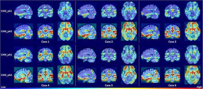
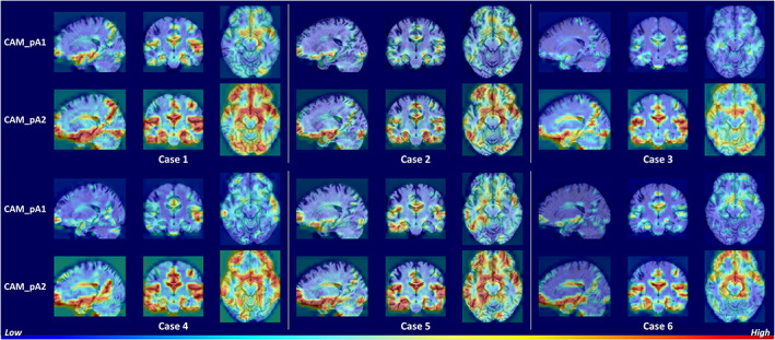
Heat maps highlighting discriminative regions of MCI conversion prediction (subjects with pMCI). The rows correspond to heat maps generated using different feature maps. The areas with warmer colors have higher discriminative contributions
Figure 3 shows similar discriminative regions across different AD subjects. The highlighted regions including hippocampus, amygdala, ventricle, frontal lobe, inferior temporal gyrus, superior temporal sulcus, parieto‐occipital sulcus, and Sylvian fissure are known to contribute to AD diagnosis (Convit et al., 2000; Ewers et al., 2011; Migliaccio et al., 2015; Scheff, Price, Schmitt, Scheff, & Mufson, 2011). Figure 4 shows the discriminative regions for MCI conversion prediction. The highlighted regions for AD and MCI subject are generally consistent. Anterior cingulate cortex, an early sign of AD (Amanzio et al., 2011), was also highlighted for some subjects. The visualizations suggest that the network is able to learn discriminative and subject‐specific features from MRI. In addition, the heat maps generated by different feature maps highlighted similar regions, while with different degrees of emphasis. This demonstrates that the pA‐blocks can attend to different correlations and capture enriched features.
4. DISCUSSION
In this study, we presented a novel end‐to‐end deep learning framework for AD classification and MCI conversion prediction. The framework did not require any prior knowledge as guidance for training. Experiments demonstrated our proposed method's effectiveness in extracting AD‐related features in sMRI images.
4.1. Comparison with previous work
We compared the proposed method's performance with other sMRI‐based CAD methods. Considering the utilization of different datasets because of subject selection criteria, sMRI preprocessing failure, and dataset partitioning, a fair comparison of these methods was impossible. However, the comparison still allowed us to make some interesting observations. In Table 5, we briefly summarize several state‐of‐the‐art results on AD classification and MCI‐to‐AD prediction using conventional machine learning or deep learning methods. It worth noting that only the results derived from sMRI are listed in the table.
TABLE 5.
A summary of state‐of‐the‐art sMRI‐based studies for AD classification and MCI conversion prediction
| Reference | Methodology | Feature engineering or prior knowledge | Subjects | AD versus NC | pMCI versus sMCI | |||||||||
|---|---|---|---|---|---|---|---|---|---|---|---|---|---|---|
| NC | sMCI | pMCI | AD | ACC (%) | SEN (%) | SPE (%) | AUC | ACC (%) | SEN (%) | SPE (%) | AUC | |||
| Eskildsen et al. (2013) | Cortical thickness + LDA | Feature engineering | 226 | 227 | 161 | 194 | 84.5 | 79.4 | 88.9 | 0.905 | 67.3 | 65.8 | 68.3 | 0.685 |
| Liu et al. (2016) | Gray matter density map + ensemble SVM | Feature engineering | 128 | 117 | 117 | 97 | 93.1 | 94.9 | 90.5 | 0.958 | 79.3 | 88.0 | 75.5 | 0.834 |
| Zhang et al. (2016) | Morphological feature + SVM | Feature engineering | 229 | ‐ | ‐ | 199 | 83.7 | 80.9 | 86.7 | ‐ | ‐ | ‐ | ‐ | ‐ |
| Moradi et al. (2015) | Gray matter density map + semi‐supervised classifier | Feature engineering | 231 | 100 | 164 | 200 | ‐ | ‐ | ‐ | ‐ | 74.7 | 88.9 | 51.6 | 0.766 |
| Suk et al. (2014) | sMRI patches + deep Boltzmann machine + SVM | ‐ | 101 | 128 | 76 | 93 | 92.4 | 91.5 | 94.6 | 0.970 | 72.4 | 36.7 | 91.0 | 0.734 |
| Lin, Tong, et al. (2018) | sMRI patches + CNN + PCA + Lasso + ELM | Prior knowledge | 229 | 139 | 169 | 188 | 88.8 | ‐ | ‐ | ‐ | 76.9 | 81.7 | 71.2 | 0.829 |
| Liu et al. (2018) | sMRI patches + CNN | Feature engineering | 452 | 465 | 205 | 404 | 91.1 | 88.1 | 93.5 | 0.959 | 76.9 | 42.1 | 82.4 | 0.776 |
| Lian et al. (2018) | sMRI patches + CNN | Prior knowledge | 429 | 465 | 205 | 358 | 90.3 | 82.4 | 96.5 | 0.951 | 80.9 | 52.6 | 85.4 | 0.781 |
| Khvostikov et al. (2018) | Hippocampal sMRI + CNN | Prior knowledge | 58 | ‐ | ‐ | 48 | 85.0 | 88.0 | 90.0 | ‐ | ‐ | ‐ | ‐ | ‐ |
| Korolev et al. (2017) | Whole brain sMRI + CNN | ‐ | 61 | ‐ | ‐ | 50 | 80.0 | ‐ | ‐ | 0.870 | ‐ | ‐ | ‐ | ‐ |
| Spasov et al. (2019) | Whole brain sMRI + CNN | ‐ | 184 | 228 | 181 | 192 | ‐ | ‐ | ‐ | ‐ | 72.0 | 63.0 | 81.0 | 0.790 |
| Ours | Whole brain sMRI + CNN | ‐ | 394 | 401 | 197 | 348 | 90.7 | 88.8 | 92.4 | 0.936 | 79.3 | 54.6 | 84.1 | 0.776 |
Most previous methods utilized a separated classifier to learn manually engineered features (Eskildsen et al., 2013; Liu et al., 2016; Moradi et al., 2015; Zhang et al., 2016). Feature extraction in these methods required either expertise regarding regions of interest or a time‐consuming process with respect to whole‐brain image intensities. Also, the separation of the feature extraction stage and classifier construction stage could compromise performance. By contrast, our method utilized CNNs to jointly build the feature extractor and classifier. Direct feature learning from sMRI improved the diagnostic performance with higher efficiency.
Some methods partially utilized neural networks (Lin, Tong, et al., 2018; Suk et al., 2014) by leveraging neural networks as a high‐level feature extractor and designing complicated classifiers to further process features extracted by the neural networks. In our study, a simple linear classifier on top of the neural network achieved good performance. This suggests that our method is able to effectively learn long‐range correlations and complexly localized patterns from image data. The deep learning methods in Lian et al. (2018) and Liu et al. (2018) required extra location proposals or detected landmarks to guide feature extraction. The location proposal and landmark detection modules were isolated from the main neural network and were highly dependent on feature engineering. By contrast, our proposed method was trained in an end‐to‐end manner with only images as input and image labels as the output. Also, because of the computationally inefficient location proposal module, the methods in Lian et al. (2018) and Liu et al. (2018) required 27 and 14 hr to train the network, respectively (both used a single GPU, that is, NVIDIA GTX TITAN 12 GB). Our method using whole‐brain MRIs was much more efficient, costing only 105 min for training. The method in Lian et al. (2018) was required to train an extra network with a structure different from the main network for generating heat maps of discriminative areas, while our framework can easily generate the heat maps without the need of changing the main network or training an extra network.
Compared with the CNN‐based methods that allow end‐to‐end training (Khvostikov et al., 2018; Korolev et al., 2017; Spasov et al., 2019), our method achieved better classification performance. This suggests that our method captures more informative features related to dementia. Furthermore, we evaluated our proposed framework in a strict setting. The network was trained and evaluated on two independent datasets (ADNI‐1 and ADNI‐2). This evaluation protocol was more challenging but ensured the effectiveness of the proposed frameworks.
Considering the risk of introducing subject duplication, that is, multiple scans from one subject appearing in both the training and test sets, we used only one baseline scan of each subject to train and evaluate the network; 3D sMRI volume was directly fed into the network. In addition, the MRI images in the training and test sets had a different signal‐to‐noise ratio (i.e., 1.5 T and 3 T scanners). The model learned by the proposed framework can still reliably distinguish different diagnostic groups. We also showed the models' extents of overfitting by evaluating the trained models on the training dataset. The detailed discussion about overfitting was presented in the Supplementary Materials.
4.2. Limitations and future work
Although the proposed framework achieved competitive diagnostic results, there is still room for improvement. First, we plan to utilize multimodal data to improve the current framework. Besides sMRI, functional imaging can help with disease diagnosis and biomarker discovery (Li, Yang, Lei, Liu, & Wee, 2019; Yu et al., 2019; Zhang et al., 2019). Some other studies utilized multimodal data for CAD or cognition prediction and achieved good performance (Liu et al., 2015, 2017; Peng, Zhu, Wang, An, & Shen, 2019; Wang, Liu, & Shen, 2019; Zhu et al., 2019). We could further study using multimodal neuroimaging combinations. Second, the generated heat maps only highlighted discriminative regions, and this interpretation is still too coarse to support clinical decision‐making. We aim to generate human‐comprehensible and fine‐grained visual attribution maps of disease effects, thereby taking a step closer toward CAD. To the end, we trained and evaluated our methods on two independent datasets, which were relatively large compared with those used in other CAD studies (see Table 5). However, further experiments are needed to evaluate the effectiveness of the framework in a larger population.
5. CONCLUSION
In this study, we developed an efficient deep neural network framework for AD diagnosis and MCI conversion prediction. Using the asymmetrically parallel structure, the proposed framework directly extracted global and local features in 3D sMRIs without extra guidance. The framework was lightweight and fast to train. Furthermore, we generated heat maps of disease‐related regions to aid visual interpretation. The proposed framework was evaluated on two public datasets with 1,340 subjects. The diagnostic performance was competitive with other state‐of‐the‐art methods, which require medical priors or stepwise training procedures.
CONFLICT OF INTEREST
The authors declare that they have no potential conflict of interest.
ETHICS STATEMENT
Ethics approval was obtained by the ADNI investigators. Written informed consent was obtained from all individuals participating in the study according to the Declaration of Helsinki.
Supporting information
FIGURE S1 MRI images of original size and cropped size. We choose the cropped size (144 × 176 × 144) to cover most areas of the brain, and reduce the useless computation in the background.
TABLE S1 Results for AD classification (AD vs. NC) using baseline sMRI. The models were trained on the ADNI‐1 dataset and evaluated on the ADNI‐2 dataset.
TABLE S2 Results for AD classification on the training dataset (ADNI‐1) and the test dataset (ADNI‐2), and the differences of these two results.
ACKNOWLEDGMENTS
This research received support from the National Natural Science Foundation of China (Grant No. 81871434 and 61971017), the National Key Research and Development Program of China (Grant No. 2019YFC0118602), and Beijing Natural Science Foundation (Grant No. Z200016).
Guan, H. , Wang, C. , Cheng, J. , Jing, J. , & Liu, T. (2022). A parallel attention‐augmented bilinear network for early magnetic resonance imaging‐based diagnosis of Alzheimer's disease. Human Brain Mapping, 43(2), 760–772. 10.1002/hbm.25685
Funding information National Key Research and Development Program of China, Grant/Award Number: 2019YFC0118602; National Natural Science Foundation of China, Grant/Award Numbers: 61971017, 81871434; Natural Science Foundation of Beijing Municipality, Grant/Award Number: Z200016
Endnotes
DATA AVAILABILITY STATEMENT
The dataset used and analyzed are available to other researchers’ subject to review of the request by the Scientific Committee of the study and ethics approval. All imaging, demographics, and neuropsychological data used in this article are publicly available and were downloaded from the ADNI website (adni.loni.usc.edu). Upon request, we will provide a list of ADNI participant identifications for replication purposes.
REFERENCES
- Amanzio, M. , Torta, D. M. , Sacco, K. , Cauda, F. , D'Agata, F. , Duca, S. , … Geminiani, G. C. (2011). Unawareness of deficits in Alzheimer's disease: Role of the cingulate cortex. Brain, 134, 1061–1076. 10.1093/brain/awr020 [DOI] [PubMed] [Google Scholar]
- Bron, E. E. , Smits, M. , van der Flier, W. M. , Vrenken, H. , Barkhof, F. , Scheltens, P. , … Alzheimer's Disease Neuroimaging Initiative . (2015). Standardized evaluation of algorithms for computer‐aided diagnosis of dementia based on structural MRI: The CADDementia challenge. NeuroImage, 111, 562–579. 10.1016/j.neuroimage.2015.01.048 [DOI] [PMC free article] [PubMed] [Google Scholar]
- Chen, Y. , Kalantidis, Y. , Li, J. , Yan, S. , & Feng, J. (2018). A2‐nets: Double attention networks. Paper presented at the Proceedings of the 32nd Conference on Neural Information Processing Systems (NeurIPS 2018), Montréal, Canada. Retrieved from https://proceedings.neurips.cc/paper/2018/file/e165421110ba03099a1c0393373c5b43-Paper.pdf
- Convit, A. , de Asis, J. , de Leon, M. J. , Tarshish, C. Y. , De Santi, S. , & Rusinek, H. (2000). Atrophy of the medial occipitotemporal, inferior, and middle temporal gyri in non‐demented elderly predict decline to Alzheimer's disease. Neurobiology of Aging, 21, 19–26. 10.1016/s0197-4580(99)00107-4 [DOI] [PubMed] [Google Scholar]
- Davatzikos, C. , Bhatt, P. , Shaw, L. M. , Batmanghelich, K. N. , & Trojanowski, J. Q. (2011). Prediction of MCI to AD conversion, via MRI, CSF biomarkers, and pattern classification. Neurobiology of Aging, 32(2322), e19–e27. 10.1016/j.neurobiolaging.2010.05.023 [DOI] [PMC free article] [PubMed] [Google Scholar]
- Ding, Y. , Sohn, J. H. , Kawczynski, M. G. , Trivedi, H. , Harnish, R. , Jenkins, N. W. , … Franc, B. L. (2019). A deep learning model to predict a diagnosis of Alzheimer disease by using (18)F‐FDG PET of the brain. Radiology, 290, 456–464. 10.1148/radiol.2018180958 [DOI] [PMC free article] [PubMed] [Google Scholar]
- Driscoll, I. , Davatzikos, C. , An, Y. , Wu, X. , Shen, D. , Kraut, M. , & Resnick, S. M. (2009). Longitudinal pattern of regional brain volume change differentiates normal aging from MCI. Neurology, 72, 1906–1913. 10.1212/WNL.0b013e3181a82634 [DOI] [PMC free article] [PubMed] [Google Scholar]
- Eskildsen, S. F. , Coupe, P. , Garcia‐Lorenzo, D. , Fonov, V. , Pruessner, J. C. , Collins, D. L. , & Alzheimer's Disease Neuroimaging Initiative . (2013). Prediction of Alzheimer's disease in subjects with mild cognitive impairment from the ADNI cohort using patterns of cortical thinning. NeuroImage, 65, 511–521. 10.1016/j.neuroimage.2012.09.058 [DOI] [PMC free article] [PubMed] [Google Scholar]
- Ewers, M. , Sperling, R. A. , Klunk, W. E. , Weiner, M. W. , & Hampel, H. (2011). Neuroimaging markers for the prediction and early diagnosis of Alzheimer's disease dementia. Trends in Neurosciences, 34, 430–442. 10.1016/j.tins.2011.05.005 [DOI] [PMC free article] [PubMed] [Google Scholar]
- Folstein, M. F. , Folstein, S. E. , & McHugh, P. R. (1975). “Mini‐mental state”: A practical method for grading the cognitive state of patients for the clinician. Journal of Psychiatric Research, 12, 189–198. 10.1037/t07757-000 [DOI] [PubMed] [Google Scholar]
- Glorot, X. , Bordes, A. , & Bengio, Y. (2015). Deep sparse rectifier neural networks. Paper presented at the Proceedings of the International Conference on Artificial Intelligence and Statistics. (Vol. 64, pp. 315‐323). Amsterdam, Netherlands: Elsevier. 10.1016/j.neunet.2014.12.006 [DOI]
- Grabner, G. , Janke, A. L. , Budge, M. M. , Smith, D. , Pruessner, J. , & Collins, D. L. (2006). Symmetric atlasing and model based segmentation: An application to the hippocampus in older adults. In Medical image computing and computer‐assisted intervention (MICCAI) (Vol. 9, pp. 58–66). Berlin, Heidelberg: Springer. 10.1007/11866763_8 [DOI] [PubMed] [Google Scholar]
- He, K. , Zhang, X. , Ren, S. , & Sun, J. (2016a). Deep residual learning for image recognition. Paper presented at the Proceedings of the IEEE Conference on Computer Vision and Pattern Recognition (pp. 770–778). 10.1109/cvpr.2016.90 [DOI]
- He, K. , Zhang, X. , Ren, S. , & Sun, J. (2016b). Identity mappings in deep residual networks. In Leibe B., Matas J., Sebe N., & Welling M. (Eds.), Paper presented at the Proceedings of the European Conference on Computer Vision – ECCV 2016. Lecture Notes in Computer Science (Vol. 9908, pp. 630–645). Cham: Springer. 10.1007/978-3-319-46493-0_38 [DOI]
- Ioffe, S. , & Szegedy, C. (2015). Batch normalization: Accelerating deep network training by reducing internal covariate shift. arXiv preprint arXiv:1502.03167. Retrieved from https://ui.adsabs.harvard.edu/abs/2015arXiv150203167I
- Jack, J. , Petersen, R. C. , Xu, Y. C. , Waring, S. C. , O'Brien, P. C. , Tangalos, E. G. , … Kokmen, E. (1997). Medial temporal atrophy on MRI in normal aging and very mild Alzheimer's disease. Neurology, 49, 786–794. 10.1212/wnl.49.3.786 [DOI] [PMC free article] [PubMed] [Google Scholar]
- Jack, J. , Wiste, H. J. , Vemuri, P. , Weigand, S. D. , Senjem, M. L. , Zeng, G. , … Alzheimer's Disease Neuroimaging Initiative . (2010). Brain beta‐amyloid measures and magnetic resonance imaging atrophy both predict time‐to‐progression from mild cognitive impairment to Alzheimer's disease. Brain, 133, 3336–3348. 10.1093/brain/awq277 [DOI] [PMC free article] [PubMed] [Google Scholar]
- Jack, C. R., Jr. , Bernstein, M. A. , Fox, N. C. , Thompson, P. , Alexander, G. , Harvey, D. , … Weiner, M. W. (2008). The Alzheimer's Disease Neuroimaging Initiative (ADNI): MRI methods. Journal of Magnetic Resonance Imaging, 27, 685–691. 10.1002/jmri.21049 [DOI] [PMC free article] [PubMed] [Google Scholar]
- Jenkinson, M. , Beckmann, C. F. , Behrens, T. E. , Woolrich, M. W. , & Smith, S. M. (2012). FSL. Neuroimage, 62, 782–790. 10.1016/j.neuroimage.2011.09.015 [DOI] [PubMed] [Google Scholar]
- Khvostikov, A. , Aderghal, K. , Benois‐Pineau, J. , Krylov, A. , & Catheline, G. (2018). 3D CNN‐based classification using sMRI and MD‐DTI images for Alzheimer disease studies. arXiv 10.1109/cbms.2018.00067 [DOI]
- Korolev, S. , Safiullin, A. , Belyaev, M. , & Dodonova, Y. (2017). Residual and plain convolutional neural networks for 3D brain MRI classification. Paper presented at the IEEE 14th International Symposium on Biomedical Imaging (IEEE‐ISBI) (pp. 835‐838). 10.1109/isbi.2017.7950647 [DOI]
- LeCun, Y. , Bengio, Y. , & Hinton, G. (2015). Deep learning. Nature, 521, 436–444. 10.1038/nature14539 [DOI] [PubMed] [Google Scholar]
- Li, Y. , Yang, H. , Lei, B. , Liu, J. , & Wee, C. Y. (2019). Novel effective connectivity inference using ultra‐group constrained orthogonal forward regression and elastic multilayer perceptron classifier for MCI identification. IEEE Transactions on Medical Imaging, 38, 1227–1239. 10.1109/TMI.2018.2882189 [DOI] [PubMed] [Google Scholar]
- Lian, C. , Liu, M. , Zhang, J. , & Shen, D. (2018). Hierarchical fully convolutional network for joint atrophy localization and Alzheimer's disease diagnosis using structural MRI. IEEE Transactions on Pattern Analysis and Machine Intelligence, 42(4), 880–893. 10.1109/TPAMI.2018.2889096 [DOI] [PMC free article] [PubMed] [Google Scholar]
- Lin, T. Y. , RoyChowdhury, A. , & Maji, S. (2018). Bilinear convolutional neural networks for fine‐grained visual recognition. IEEE Transactions on Pattern Analysis and Machine Intelligence, 40, 1309–1322. 10.1109/TPAMI.2017.2723400 [DOI] [PubMed] [Google Scholar]
- Lin, T.‐Y. , RoyChowdhury, A. , & Maji, S. (2015). Bilinear cnn models for fine‐grained visual recognition. Paper presented at the Proceedings of the International Conference on Computer Vision (ICCV) (pp. 1449‐1457). IEEE. 10.1109/iccv.2015.170 [DOI]
- Lin, W. , Tong, T. , Gao, Q. , Guo, D. , Du, X. , Yang, Y. , … Alzheimer's Disease Neuroimaging Initiative . (2018). Convolutional neural networks‐based MRI image analysis for the Alzheimer's disease prediction from mild cognitive impairment. Frontiers in Neuroscience, 12, 777. 10.3389/fnins.2018.00777 [DOI] [PMC free article] [PubMed] [Google Scholar]
- Liu, M. , Zhang, D. , & Shen, D. (2016). Relationship induced multi‐template learning for diagnosis of Alzheimer's disease and mild cognitive impairment. IEEE Transactions on Medical Imaging, 35, 1463–1474. 10.1109/TMI.2016.2515021 [DOI] [PMC free article] [PubMed] [Google Scholar]
- Liu, M. , Zhang, J. , Adeli, E. , & Shen, D. (2018). Landmark‐based deep multi‐instance learning for brain disease diagnosis. Medical Image Analysis, 43, 157–168. 10.1016/j.media.2017.10.005 [DOI] [PMC free article] [PubMed] [Google Scholar]
- Liu, M. , Zhang, J. , Yap, P. T. , & Shen, D. (2017). View‐aligned hypergraph learning for Alzheimer's disease diagnosis with incomplete multi‐modality data. Medical Image Analysis, 36, 123–134. 10.1016/j.media.2016.11.002 [DOI] [PMC free article] [PubMed] [Google Scholar]
- Liu, S. , Liu, S. , Cai, W. , Che, H. , Pujol, S. , Kikinis, R. , … Adni . (2015). Multimodal neuroimaging feature learning for multiclass diagnosis of Alzheimer's disease. IEEE Transactions on Biomedical Engineering, 62, 1132–1140. 10.1109/TBME.2014.2372011 [DOI] [PMC free article] [PubMed] [Google Scholar]
- Livingston, G. , Sommerlad, A. , Orgeta, V. , Costafreda, S. G. , Huntley, J. , Ames, D. , … Mukadam, N. (2017). Dementia prevention, intervention, and care. The Lancet, 390, 2673–2734. 10.1016/S0140-6736(17)31363-6 [DOI] [PubMed] [Google Scholar]
- Loshchilov, I. , & Hutter, F. (2017). Fixing weight decay regularization in Adam. arXiv. 10.1063/1.5130967 [DOI]
- Luo, W. , Li, Y. , Urtasun, R. , & Zemel, R. (2018). Understanding the effective receptive field in deep convolutional neural networks. Advances in Neural Information Processing Systems (pp. 4898‐4906). 10.1109/cvpr.2018.00376 [DOI]
- Migliaccio, R. , Agosta, F. , Possin, K. L. , Canu, E. , Filippi, M. , Rabinovici, G. D. , … Gorno‐Tempini, M. L. (2015). Mapping the progression of atrophy in early‐ and late‐onset Alzheimer's disease. Journal of Alzheimer's Disease, 46, 351–364. 10.3233/JAD-142292 [DOI] [PMC free article] [PubMed] [Google Scholar]
- Moradi, E. , Pepe, A. , Gaser, C. , Huttunen, H. , Tohka, J. , & Alzheimer's Disease Neuroimaging Initiative . (2015). Machine learning framework for early MRI‐based Alzheimer's conversion prediction in MCI subjects. NeuroImage, 104, 398–412. 10.1016/j.neuroimage.2014.10.002 [DOI] [PMC free article] [PubMed] [Google Scholar]
- Pawlowski, N. , Ktena, S. I. , Lee, M. C. , Kainz, B. , Rueckert, D. , Glocker, B. , & Rajchl, M. (2017). DLTK: State of the art reference implementations for deep learning on medical images. arXiv, 469‐477. 10.1007/978-3-319-66182-7_54 [DOI]
- Peng, J. , Zhu, X. , Wang, Y. , An, L. , & Shen, D. (2019). Structured sparsity regularized multiple kernel learning for Alzheimer's disease diagnosis. Pattern Recognition, 88, 370–382. 10.1016/j.patcog.2018.11.027 [DOI] [PMC free article] [PubMed] [Google Scholar]
- Rathore, S. , Habes, M. , Iftikhar, M. A. , Shacklett, A. , & Davatzikos, C. (2017). A review on neuroimaging‐based classification studies and associated feature extraction methods for Alzheimer's disease and its prodromal stages. NeuroImage, 155, 530–548. 10.1016/j.neuroimage.2017.03.057 [DOI] [PMC free article] [PubMed] [Google Scholar]
- Scheff, S. W. , Price, D. A. , Schmitt, F. A. , Scheff, M. A. , & Mufson, E. J. (2011). Synaptic loss in the inferior temporal gyrus in mild cognitive impairment and Alzheimer's disease. Journal of Alzheimer's Disease, 24, 547–557. 10.3233/JAD-2011-101782 [DOI] [PMC free article] [PubMed] [Google Scholar]
- Spasov, S. , Passamonti, L. , Duggento, A. , Lio, P. , Toschi, N. , & Alzheimer's Disease Neuroimaging Initiative . (2019). A parameter‐efficient deep learning approach to predict conversion from mild cognitive impairment to Alzheimer's disease. NeuroImage, 189, 276–287. 10.1016/j.neuroimage.2019.01.031 [DOI] [PubMed] [Google Scholar]
- Srivastava, N. , Hinton, G. , Krizhevsky, A. , Sutskever, I. , & Salakhutdinov, R. (2014). Dropout: A simple way to prevent neural networks from overfitting. Journal of Machine Learning Research, 15, 1929–1958. 10.1145/3065386 [DOI] [Google Scholar]
- Suk, H. I. , Lee, S. W. , Shen, D. , & Alzheimer's Disease Neuroimaging Initiative . (2014). Hierarchical feature representation and multimodal fusion with deep learning for AD/MCI diagnosis. NeuroImage, 101, 569–582. 10.1016/j.neuroimage.2014.06.077 [DOI] [PMC free article] [PubMed] [Google Scholar]
- Suk, H. I. , Lee, S. W. , Shen, D. , & Alzheimer's Disease Neuroimaging Initiative . (2017). Deep ensemble learning of sparse regression models for brain disease diagnosis. Medical Image Analysis, 37, 101–113. 10.1016/j.media.2017.01.008 [DOI] [PMC free article] [PubMed] [Google Scholar]
- Szegedy, C. , Liu, W. , Jia, Y. , Sermanet, P. , Reed, S. , Anguelov, D. , … Rabinovich, A. (2015). Going deeper with convolutions. Paper presented at the Proceedings of the IEEE Conference on Computer Vision and Pattern Recognition (CVPR) (pp. 1‐9). 10.1109/cvpr.2015.7298594 [DOI]
- Tong, T. , Gao, Q. , Guerrero, R. , Ledig, C. , Chen, L. , Rueckert, D. , & Initiative, A. D. (2017). A novel grading biomarker for the prediction of conversion from mild cognitive impairment to Alzheimer's disease. IEEE Transactions on Biomedical Engineering, 64, 155–165. 10.1109/TBME.2016.2549363 [DOI] [PubMed] [Google Scholar]
- Tran, D. , Bourdev, L. , Fergus, R. , Torresani, L. , & Paluri, M. (2015). Learning spatiotemporal features with 3d convolutional networks. Paper presented at the Proceedings of the International Conference on Computer Vision (ICCV) (pp. 4489‐4497). 10.1109/iccv.2015.510 [DOI]
- Vemuri, P. , Wiste, H. J. , Weigand, S. D. , Shaw, L. M. , Trojanowski, J. Q. , Weiner, M. W. , … Alzheimer's Disease Neuroimaging Initiative . (2009). MRI and CSF biomarkers in normal, MCI, and AD subjects: Diagnostic discrimination and cognitive correlations. Neurology, 73, 287–293. 10.1212/WNL.0b013e3181af79e5 [DOI] [PMC free article] [PubMed] [Google Scholar]
- Vieira, S. , Pinaya, W. H. , & Mechelli, A. (2017). Using deep learning to investigate the neuroimaging correlates of psychiatric and neurological disorders: Methods and applications. Neuroscience and Biobehavioral Reviews, 74, 58–75. 10.1016/j.neubiorev.2017.01.002 [DOI] [PubMed] [Google Scholar]
- Wang, H. , Wang, Z. , Du, M. , Yang, F. , Zhang, Z. , Ding, S. , … Hu, X. (2020). Score‐CAM: Score‐weighted visual explanations for convolutional neural networks. Paper presented at the 2020 IEEE/CVF Conference on Computer Vision and Pattern Recognition Workshops (CVPRW), 111–119. 10.1109/cvprw50498.2020.00020 [DOI]
- Wang, P. , Liu, Y. , & Shen, D. (2019). Flexible locally weighted penalized regression with applications on prediction of Alzheimer's Disease Neuroimaging Initiative's clinical scores. IEEE Transactions on Medical Imaging, 38, 1398–1408. 10.1109/TMI.2018.2884943 [DOI] [PMC free article] [PubMed] [Google Scholar]
- Weimer, D. L. , & Sager, M. A. (2009). Early identification and treatment of Alzheimer's disease: Social and fiscal outcomes. Alzheimers Dement, 5, 215–226. 10.1016/j.jalz.2009.01.028 [DOI] [PMC free article] [PubMed] [Google Scholar]
- Yu, R. , Qiao, L. , Chen, M. , Lee, S. W. , Fei, X. , & Shen, D. (2019). Weighted graph regularized sparse brain network construction for MCI identification. Pattern Recognition, 90, 220–231. 10.1016/j.patcog.2019.01.015 [DOI] [PMC free article] [PubMed] [Google Scholar]
- Zaharchuk, G. , Gong, E. , Wintermark, M. , Rubin, D. , & Langlotz, C. P. (2018). Deep learning in neuroradiology. American Journal of Neuroradiology, 39, 1776–1784. 10.3174/ajnr.A5543 [DOI] [PMC free article] [PubMed] [Google Scholar]
- Zhang, H. , Cisse, M. , Dauphin, Y. N. , & Lopez‐Paz, D. (2017). Mixup: Beyond empirical risk minimization. arXiv, 504‐519. 10.1007/978-3-030-01231-1_31 [DOI]
- Zhang, J. , Gao, Y. , Gao, Y. , Munsell, B. C. , & Shen, D. (2016). Detecting anatomical landmarks for fast Alzheimer's disease diagnosis. IEEE Transactions on Medical Imaging, 35, 2524–2533. 10.1109/TMI.2016.2582386 [DOI] [PMC free article] [PubMed] [Google Scholar]
- Zhang, Y. , Zhang, H. , Chen, X. , Liu, M. , Zhu, X. , Lee, S. W. , & Shen, D. (2019). Strength and similarity guided group‐level brain functional network construction for MCI diagnosis. Pattern Recognition, 88, 421–430. 10.1016/j.patcog.2018.12.001 [DOI] [PMC free article] [PubMed] [Google Scholar]
- Zhu, Y. , Zhu, X. , Kim, M. , Yan, J. , Kaufer, D. , & Wu, G. (2019). Dynamic hyper‐graph inference framework for computer‐assisted diagnosis of neurodegenerative diseases. IEEE Transactions on Medical Imaging, 38, 608–616. 10.1109/TMI.2018.2868086 [DOI] [PMC free article] [PubMed] [Google Scholar]
Associated Data
This section collects any data citations, data availability statements, or supplementary materials included in this article.
Supplementary Materials
FIGURE S1 MRI images of original size and cropped size. We choose the cropped size (144 × 176 × 144) to cover most areas of the brain, and reduce the useless computation in the background.
TABLE S1 Results for AD classification (AD vs. NC) using baseline sMRI. The models were trained on the ADNI‐1 dataset and evaluated on the ADNI‐2 dataset.
TABLE S2 Results for AD classification on the training dataset (ADNI‐1) and the test dataset (ADNI‐2), and the differences of these two results.
Data Availability Statement
The dataset used and analyzed are available to other researchers’ subject to review of the request by the Scientific Committee of the study and ethics approval. All imaging, demographics, and neuropsychological data used in this article are publicly available and were downloaded from the ADNI website (adni.loni.usc.edu). Upon request, we will provide a list of ADNI participant identifications for replication purposes.