An empowered AdaBoost algorithm implementation: A COVID-19 dataset study

Abstract

The Covid-19 outbreak, which emerged in 2020, became the top priority of the world. The fight against this disease, which has caused millions of people’s deaths, is still ongoing, and it is expected that these studies will continue for years. In this study, we propose an improved learning model to predict the severity of the patients by exploiting a combination of machine learning techniques. The proposed model uses an adaptive boost algorithm with a decision tree estimator and a new parameter tuning process. The learning ratio of the new model is promising after many repeated experiments are performed by using different parameters to reduce the effect of selecting random parameters. The proposed algorithm is compared with other recent state-of-the-art algorithms on UCI data sets and a recent Covid-19 dataset. It is observed that competitive accuracy results are obtained, and we hope that this study unveils more usage of advanced machine learning approaches.

1. Introduction

Humankind has endeavoured to make sense of the events around it since the first years of its existence. Machine learning (ML) algorithms have helped much understand and predict unknown events. Predictions have gained dimensions and approaches for more complex and numerous data (Lu, 2019, Shhadat, Hayajneh, & Al-Sharif, 2020). A group of input variables evaluates the predicted variable (dependent variable in statistics). With these variables, many tools such as trees, different regression techniques, nearest neighbours, boosting algorithms, etc., have been studied to put forward a model that maps the input variables to output classes. However, studies do not provide a desired level of accuracy most of the time. This study originates from such a need and requirement. It tries to propose a model which achieves a mapping close to optimum in a short period.

Usage of ML algorithms increases the computing power and accuracy, especially ensemble methods come forward at this point (Seni & Elder, 2010). The ensemble methods enable us to train multiple models using the same learning algorithm. The proposed algorithm of this study is an excellent example of this technique. Besides that, a model having an integrated ensemble algorithm is more likely to get the minimum error and higher accuracy levels.

Freund and Shapire introduced the Adaptive Boosting (AdaBoost) algorithm in (Freund, 1995) then improved it (Freund & Schapire, 1997). In the algorithm, they used so-called “weak” classifiers to perform better performance which can lead the AdaBoost into a powerful, high-performance algorithm. They developed an exponential loss function to update the weights. After that, many studies have been made and presented, and some of them are as in (Schapire, 2003, Souza and Matwin, 2012).

The AdaBoost is a popular classification algorithm. During the training phase, the distribution weight of the sample is increased as the error rate increases, and oppositely as it decreases, the new distribution weight is reduced. Then samples are continually trained with the unknown distribution weights. The aim is to have strong feedback by reducing the next machine’s error and reaching better accuracy rates in the end. The process of the AdaBoost algorithm can be found easily, and one sample research is in (Lu, Hu, & Bai, 2015).

Almost one and a half year ago, the World Health Organization (WHO) stated to the world that COVID-19 is a pandemic. The rapid spread of the disease around the globe brought it necessary to take many measures immediately. Unfortunately, the final figures are embarrassing since over 178 million people are infected (confirmed) and over 3.8 million dead all over the world according to (Who coronavirus (covid-19) dashboard) by the end of March 2021. The main goal of this study is to support and contribute the solution to an epidemic. The virus spreads mainly through saliva droplets. After being infected, the disease causes pneumonia in the lungs, which cause difficulty in breathing. The most common symptoms in COVID-19 patients were recorded as fever and cough as in (Lai, Shih, Ko, Tang, & Hsueh, 2020).

The proposed model of the study is an empowered ensemble method using an adaptive boost strategy. The algorithm gets “Decision Tree” as the base classifier. In a standard AdaBoost model, predictions are made on the training set, and the weight of input is updated due to the error rate. Then a second classifier is trained using the updated weight, and it makes predictions on the training set again. This feedback results in a remarkable decrease in error. This procedure goes on in this way up to the end.

Briefly, a machine-learning algorithm has been proposed and tuned for quick and effective learning here. This tuning process is done for empowering the primary model using an adaptive boosting approach. One of the best capabilities of the proposed algorithm is that it obtains and gets the results in a moderate computer in short periods due to other known AI and ML algorithms. The way the proposed algorithm works is that it drops into filtering methods since it is related to the correlations between the input and the output classes.

The experiments are conducted on two datasets. In the first part, well-known UCI-datasets (Uci machine learning repository: data sets) are used, and even this part is also divided into two sections. In the first section, ensemble algorithms are shown using two sample datasets. This section shows the reason for selecting the adaptive boosting approach. Then in the second section of the first part, the proposed algorithm is compared with known sample ML datasets taken from (Datasets: Feature selection @ asu; Uci machine learning repository: data sets). This is done for presenting the accuracy rates of all compared algorithms using these datasets. Finally, in the second part, the proposed algorithm is compared with other known and recent algorithms to present the aim of this study.

This paper is organized as follows. Section 2 presents the recent studies on the topic. Section 3 shows the proposed algorithm after brief information on AdaBoost Algorithm and Decision Trees. Then Section 4 presents the results of this study in three consecutive subsections. In the first one, comparisons of all ensemble methods, in the second one comparisons of known and recent algorithms, and the third one comparisons of other state-of-the-art algorithms are compared. Finally, Section 5 presents conclusions and future works of the study.

2. Related work

Although ML algorithms have major sub-fields, supervised learning studies are the most known and popular ones. In this method, algorithms are mainly categorized into two main types,$\mathit{filter}$ and $\mathit{wrapper}$ algorithms. The main difference between these two algorithms is that filtering algorithms try to evaluate the correlation with the output class. In contrast, wrapper methods try to find out a subset of input variables to use. There are also hybrid approaches as well in the literature.

Feature selection methods, most of which have been used and studied mainly for analysis, classification, categorization, pattern detection, etc., are popular in supervised learning. Some recent studies on classification are presented in (Sevinc, 2019, Sevinç and Dökeroglu, 2019). Feature selection techniques are done by extreme learning machine (Huang, Zhou, Ding, & Zhang, 2012) and improved by GA methodologies for better performance. A similar GA is presented in (Karakaya, 2017). The aim is to find a generic solution in a reasonable amount of time after optimizing an improved GA. Similarly, in (Deniz et al., 2017, Dokeroglu and Sevinc, 2019), some filtering mechanisms and methodologies supported by extreme learning machines have been developed and experimented with for feature subset selection. These studies are good examples of filter-based feature selection approach while Xue et al. (Xue et al., 2019) presents a wrapper feature selection algorithm for classification. They proposed a re-weighted multi-view algorithm which allowed multiple relevant views for better accuracy. As a hybrid approach, Zhu et al. proposed a hybrid filter and wrapper feature selection algorithm with a combination of genetic algorithm (GA) and local search (LS) in (Zhu, Ong, & Dash, 2007).

Additionally, there are other algorithms, such as meta-heuristic algorithms, in the literature. Artificial Bee Colony, Bacterial Foraging, Bat Algorithm, Gary wolf, whale optimization, etc., are involved in this group. These methodologies aim to reach better classification performances by upgrading some parameters and implementing specific feature selection techniques. A survey is presented in (Dokeroglu, Sevinc, Kucukyilmaz, & Cosar, 2019) and two additional study is presented in (Mirjalili, 2015, Li et al., 2020). The final two studies from which this study benefited are binary classification algorithms that affected and developed from the movements of dragonflies.

If it comes to the ML algorithm for classification, it is a vast field and still developing. You can find many ML algorithms for regression and classification problems. The most popular ML website is presented in (Api reference) in which python base classes and utility functions are listed. One can easily create unique models by using integrated most common ML algorithms and get remarkable results.

As a research study on ML algorithms, a prominent one can be found in (Souza & Matwin, 2012). It is one of the initial examples of the Adaptive Boost (AdaBoost) algorithm. The authors used resampling with substitution instead of the re-weighting approach for reaching a good “weak learner”. They claimed that the proposed model produced the slightest error for specific weight distribution by this process. Because the weaker learner you get, the lower error rate you reach. In another interesting study in (Bai, Xie, Wang, Zhang, & Li, 2021), a similar AdaBoost algorithm is put forward which is close to the approach in here. Their model has three elements mainly and the learning performance of the model is reinforced by the AdaBoost approach. Finally, it is claimed that the proposed model overwhelms all the comparison models in terms of root-mean-square error, threshold statistics, and residuals analysis. It is also added that they successfully improve the sensitivity and regression capacity of the model by handling the rough knowledge synchronously with their AdaBoost methodology.

Among ML algorithms, Ensemble algorithms must be taken into consideration since they have an essential role in learning methodology. In (Kiziloz, 2021), five popular ensemble methods are implemented for feature selection, and models are run on known datasets from (Uci machine learning repository: data sets). When used as the only algorithm in the model, it has been reported that it executes fast; however, when they are used together and integrated, they perform better in terms of accuracy. This is believed to be reasonable, and this methodology is also performed in this study. Also in (Priore, Ponte, Puente, & Gómez, 2018), a scheduling based using ensemble methods of machine learning algorithms has been presented. They deal with the scheduling problem and try to improve the result by considering the recommendations made by different ensemble methods of ML algorithms. Thus, they try to obtain a conceptual evolution in the design of control systems. In addition, the study in (Albadr et al., 2020) tries to identify the effectiveness of detecting COVID-19 using chest X-ray images by integrating Extreme Learning Machine with genetic algorithm evolutionary capabilities.

Ensemble methods are so attractive that you can encounter easily as in a typical combinatorial optimization problem, a Dynamic Vehicle Routing Problem (DVRP) studied in (Wang, Liao, Li, Yan, & Chen, 2021). The authors try to find a solution to the problem with time windows constraint. Finally, they construct a multi-objective optimization model for the problem and improve it by an ensemble learning method. They claim that the ensemble learning model can help to improve the capability of adapting to new environments with different dynamic conditions.

Similar to these studies, there are many other studies such as in (Guz et al., 2010, Jabri et al., 2018, Khan et al., 2020). All these studies aim to show the power of AdaBoost algorithm, especially in binary classification problems. After tuning and making repeated experiments on a real dataset, i.e. Covid-19, we also try to present the success of the proposed model against best known and recent state-of-the-art algorithms.

3. Proposed algorithm

In this part, a tuned Adaptive Boost (AdaBoost) Algorithm is presented. A model that is empowered by a classifier is a candidate solution to predict and solve such regression and classification problems with higher success.

Another aim of the algorithm is to reach the possible best accuracy within a short period. Execution times will also be mentioned here since it is an essential issue for any machine learning algorithm. The results of the experiments are the averages of 10 independent runs of program executions to get rid of any randomness effect.

Adaptive Boosting (AdaBoost), first introduced by (Freund & Schapire, 1997) is briefly a general ensemble method that creates a strong classifier by using a number of weak classifiers. The algorithm starts with a weak learner, weighting each example equally. This is obtained by applying weights $w_1,w_2,\dots w_N$ to each training sample, which is called boosting iterations. At the beginning, all the weights are equally set to $w_i=\frac{1}{N}$. Then a weak learner on the original data is trained by training dataset. At each iteration, sample weights are updated, and this continues as it is reapplied to the data again up to the end. At each step, as the correct predictions are made, the weight of the training example is decreased, and oppositely the weight is increased if the model incorrectly predicted it. In other words, misclassified examples get their weights increased for the next round(s), while correctly classified ones get their weights decreased. Finally, predictions are integrated with a weighted majority sum to get the final prediction.

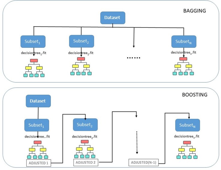
Machine learning models generally suffer from bias or variances, and many studies are proposed to minimize this effect. Ensemble learning methods are good examples to mention related to the point. These methodologies are known to make training and predictions based on different models. Then by combining them, these models tend to have less bias and be less data-sensitive. The two most popular ensemble methods are bagging and boosting.

• •Bagging: Its name comes from Bootstrap AGGregatINGand mostly applies the decision tree method as a Bootstrap variance. Bagging trains all individual models parallel and each model is trained by a random subset of the dataset. As a result, the average of all the predictions from different trees are evaluated and unbiased when compared to a single decision tree
• •Boosting: This method trains a group of individual models in a sequential way. Each individual model gets a feedback from mistakes made by the previous model. Subsequent trees are re-trained at every step since the goal is to solve the absolute error caused by the previous tree. This method shows how AdaBoost works mainly.

A sample illustration of these methods can be seen in Fig. 1 . As mentioned, the proposed algorithm uses Boosting strategy and it can be seen that a high learning rate is more probable.

Fig. 1.

Bagging and Boosting Illustration.

3.1. Adaptive boost algorithm

Though multi label classification is possible, because of Covid-19 data set, a binary classification will be shown. Each data is presented and labeled as in Eq. 1

$$(x_1,y_1),(x_2,y_2),\dots ,(x_k,y_k)$$ (1)

where k is training data set size, $x_i\in T$ and $y_i\in${-1, 1}. T represents the training data and the set {-1, 1} binary class labels for the data elements. Each training data sample $x_i$ can be a point in a multidimensional feature space.

AdaBoost by itself implements a probability distribution over all the training samples. This distribution is modified by iterations with a new weak classifier to the data. In this study, the probability distribution is denoted as $D_t(x_i)$ and t refers to the successive iterations of the algorithm. The weak classifier chosen for the iteration t is denoted by $h_t$. Then the class label assigned by $x_i$ is presented by $h_t(x_i)$. By comparing $h_t(x_i)$ with $y_i$ for i  = 1, 2, …,k, there will be an error ${∊}_t$, which is called as the classification error rate for the classifier $h_t$.

Each candidate classifier is trained during iterations using a sub-sampling of all of the training data as provided by the probability distribution $D_t(x)$. As a result, the higher the probability $D_t(x)$ for a given training sample x, the greater the chance that it will be chosen for training the candidate classifier h(t). The selection of $h_t$ is essential since among all different possible values, the one that minimizes the misclassification rate ${∊}_t$ must be chosen. For example, a weak classifier is primarily a single feature that is simply a threshold in most AdaBoost implementations.

The other important point for AdaBoost algorithm is the trust level ${\alpha }_t$, of weak classifier in which we trust. As mentioned clearly before, the bigger the value of error, ${∊}_t$ for a classifier, the lower the trust must be. The relation between ${\alpha }_t$ and ${∊}_t$ is shown in Eq. 2

$${\alpha }_t=\frac{1}{2}\mathit{ln}\frac{1-{∊}_t}{{∊}_t}$$ (2)

If the error rate, ${∊}_t$, gets closer to 1 starting from 0, the trust level of the candidate classifier h(t) will get a value in the scale of $-\infty$ and $\infty$. ${∊}_t$ being close to 1 means that the weak classifier fails almost completely on the overall training dataset, and ${∊}_t$ being close to 0 means that your weak classifier is a powerful classifier as also stated in (Cao, Miao, Liu, & Gao, 2014)

A final classifier H is obtained at the end. After k iterations, H classifier in AdaBoost algorithm is evaluated as in Eq. 3

$$H(x)=\mathit{sign}\left({\displaystyle \sum _{t=1}^k}{\alpha }_t.h_t(x)\right)$$ (3)

where x is the new data element which denotes the information strength in the training data. For example, in binary classification if H(x) is positive, then the predicted class is 1, otherwise, it is −1.

The classifier presents a weighted aggregation produced by the individual weak classifiers. Thus, in the end, a single strong, weak classifier can dominate over several not-so-strong weak classifiers with the highest trust factor ${\alpha }_t$ among others. A fundamental AdaBoost algorithm is explained in (Schapire, 2003), and related python libraries can be easily found in (Api reference).

The proposed AdaBoost algorithm of this study works through the following steps;

• 1.Initially, Adaboost creates and assigns training and test subsets randomly.
• 2.It trains the model through iterations by selecting the training set.
• 3.It assigns the higher weight to wrong classified observations so that in the next iteration, these observations will get a high probability for classification.
• 4.Algorithm assigns the weight to the classifier after each iteration due to the tuned Decision Tree classifier.
• 5.The whole process continues until the complete training data fits without any error or reaches a maximum number of estimators.
• 6.To classify, perform a “vote” among classifiers and decide the output due to the model built.

3.2. Decision trees

Decision trees are well-known and popular for classification problems. Their popularity mainly originates from the similarity to that of standard human brain’s making decisions. Being a supervised machine learning algorithm, a decision tree includes a series of sequential decisions given for reaching a specific result. This mechanism is adopted for reaching better accuracy in the tests. The decision tree classifier evaluates due to the majority over many decisions and then makes the decision.

The decision tree algorithm starts with attribute election. For this, Attribute Selection Measure (ASM) split records and provides a rank and weight for the dataset features. Gini index and information gain are the most popular methods for ASM. According to these methods, features take place at the root node or the internal nodes; then, evaluation is done. More information about the indexes can be found in (Raileanu & Stoffel, 2004).

Different decision tree algorithms use gini, entropy, or a combination of both. Gini index and entropy are the criteria for evaluating information gain. Decision tree algorithms use this value to split a node. These two measures show the noise/impurity degree of a node. For example, if a node has multiple classes, it indicates impurity, and oppositely if a node has only one class, it means it is pure. Finally, a decision tree is a graph-based solution to a problem representing all possible solutions to a trial by decisions based on given conditions.

3.3. Tuning AdaBoost with decision tree classifier

The proposed algorithm here is called Empowered ADAboost with Decision Tree (E-ADAD) method. The algorithm mainly uses tuning parameters of related python libraries defined in the “sklearn” package. Python libraries have a wide range of capabilities by simply making function calls to manage and achieve a wide range of abilities. Many types of different models can be developed and used for other purposes for future problems.“Decision Tree” classifier has been used as the estimator and the “gini” method has been implemented by this classifier. In a binary classification problem such as the Covid-19 dataset, gini criterion is more popular and powerful. Its formula is presented in Eq. 4.

$$\mathit{Gini}=1-{\displaystyle \sum _{i=1}^n}{p}^2(c_i)$$ (4)

where $p(c_i)$ is the probability of class $c_i$ in that node. Gini Index suggests a two-way split for the attributes and thus we can compute a weighted sum of the impurity for each partition separately.

The classifier of E-ADAD model definition is given below;

$$\begin{array}{cc}& \mathrm{clf}=\mathrm{AdaBoostClassifier}(\\ & \mathrm{DecisionTreeClassifier}\left(\mathrm{criterion}=’\mathrm{gini}’,\max \_d\mathrm{epth}=4\right),\\ & \mathrm{learning}\_ra\mathrm{te}=0.9)\end{array}$$

Though it is not shown, there is a split strategy in the constructor, namely “best”. It is assigned by default. Additionally, another important parameter is the “maximum depth of the tree”. A higher maximum depth value causes overfitting, while a lower one causes underfitting. This value is assigned as “4” as seen in the model definition.

E-ADAD uses the “learning rate” parameter, which is denoted generally as $\alpha$, shows the speed of learning that the model achieves. However, slower learning brings forward another significant point. A low learning rate will take much time and more probability to converge or get stuck in an undesirable local minimum. However, a higher one makes the learning jump over minima. In this study, 0.8 $⩽\alpha ⩽$1.0 is selected for E-ADAD since this range was observed to be more appropriate during the tests. Another point is that different $\alpha$ values being in the range are taken for different datasets.

Number of estimators is another parameter that affects accuracy. The default value is 50, and this number is the point where boosting is terminated. The default value is chosen and used for E-ADAD.

Finally, $\mathit{algorithm}\{\prime \mathit{SAMME}.R\prime \}$ is assigned by default. It is also clearly emphasized in the study (Hastie, Rosset, Zhu, & Zou, 2009) that the two-class AdaBoost builds an additive model to approximate the two-class Bayes rule. The SAMME.R is a natural and clean multi-class extension of the two-class AdaBoost algorithm. In other words, by its nature SAMME/SAMME.R adapts to the philosophy of boosting, and it is strongly believed that it is a powerful method in two-class predictions.

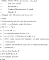
E-ADAD algorithm is presented below;

Algorithm 1

E-ADAD Algorithm

Due to result of AdaBoost algorithm, results are obtained on the test dataset and according to supervised learning methodology, success rate is evaluated.

4. Experimental results

4.1. Comparison among other ensemble algorithms

The experiments are executed on a standard laptop Windows-10 machine. It has an i7 CPU (i7-5700HQ CPU @ 2.70 GHz) and 16 GB of memory. The code is implemented in Jupyter-notebook Version 3.0.0. All coding is in Python 3.6 version and *.ipynb format.

Ensemble algorithms are well-known among ML algorithms. They have an essential role since they are flexible and integrated by different types of estimators. These ensemble estimators are ideal for regression and classification problems since they are capable of reducing bias and variance to increase the performance of models.

Decision trees are the ones that are mostly integrated with ensemble algorithms. They are easy to understand and produce remarkable results in a world full of algorithms that look like a black box. Even after combining several models, ensemble methods improve learning much, as also stated in (Kiziloz, 2021).

Adaptive Boost (Adaboost) Algorithm: AdaBoost is powerful to arrange a set of weak classifiers in a sequence in which each weak classifier is the best choice for a classifier at that point for rectifying the errors made by the previous classifier. Boosting means arranging a set of weak classifiers in a sequence in which each weak classifier is the best choice for a classifier to rectify the errors made by the previous classifier.

AdaBoost can improve its ability to learn from past errors since it has the theoretical guarantee that as more weak classifiers are put into use, the final misclassification rate must be made arbitrarily small. Additionally, the AdaBoost approach has a bound on the generalization error. This means it will not ever increase since the updated weight will decrease. Finally, this method constitutes the origin of this study.

Random Forest Algorithm: Random Forest is a tree-based machine learning algorithm that integrates the solving capability of multiple decision trees. As the name suggests, this approach proposes a “forest” of trees. Decision trees are randomly created, and each node in the tree works on a random subset of features to predict the output. Then this random forest collects and integrates the result of individual decision trees, then evaluates the final output.

In the experiments, data sets have been divided into train and test subsets with different proportions obtained by randomly selected same subsets. This is done for getting rid of the effect of any time randomness. In other words, random_state parameter must be set to a value in order not to get different results after each execution. This is important because when we use $\mathit{random}\_\mathit{state}=\mathit{some}\_\mathit{number}$ parameter, this means that each split will be random but the same every time. It provides us to work on the same split as the first time it is assigned.

A sample code using sci-kit for splitting the dataset is given below;

$$\begin{array}{cc}& \mathrm{from}\mathrm{sklearn}.\mathrm{model}.s\mathrm{election}\mathrm{import}\mathrm{train}\_\mathrm{test}\_\mathrm{split}\\ & X\_\mathrm{train},X\_\mathrm{test},y\_\mathrm{train},y\_\mathrm{test}=\\ & \mathrm{train}\_\mathrm{test}\_s\mathrm{plit}\left(X,y,\mathrm{test}\_\mathrm{size}=0.25,\mathrm{random}\_\mathrm{state}=0\right)\end{array}$$

According to that code, the training size is 75% of data while the test size is 25%. The split is first randomly done and is the same for each run. That means the initial random selection is the same for each run/split. $\mathit{random}\_\mathit{state}=0$ means that the data will be randomly split, but the same random parts will be selected. The number “0” has no impact on this.

Histogram-based Gradient Boosting: Histogram-based Gradient Boosting approach is very similar to that of Gradient Boosting except for the compatibility with the dataset. This classification tree estimator is relatively faster than GradientBoostingClassifier for big datasets (number of samples $⩾$10000).

In this algorithm, each predictor is to be improved by reducing the errors due to its predecessor. However, Gradient Boosting fits a new predictor of the previous predictor’s residual errors instead of providing a predictor on the data at each iteration.

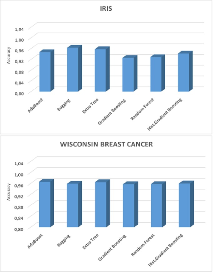
Finally, ensemble algorithms are compared to show the best one. The results can be seen in Fig. 2 . For all the algorithms, “Iris” and “Wisconsin Breast Cancer” datasets have been used. These datasets are mostly used ones while “Iris” is multi-class classification and “Wisconsin Breast Cancer” is a two-class classification problem. The reason for selecting these two common datasets is to show a clear distinction among the candidate algorithms.

Fig. 2.

Accuracy Rates of Ensemble Algorithms.

All ensemble classification algorithms are experienced on these datasets in Fig. 2. Though all the results are close to each other AdaBoost algorithm is slightly more successful when compared to others. Esp. in a binary class classification problem, AdaBoost Algorithms are more successful, as seen in “Wisconsin Breast Cancer”. It can be observed that it is about 5% better than the average of the rest algorithms.

4.2. Comparison with state-of-the-art algorithms

The study in (Too & Mirjalili, 2021) is a very recent and remarkable one in the literature. Binary Dragonfly Algorithm is discussed and used, then some parameters are changed, and a new algorithm, hyper learning binary dragonfly algorithm (HLBDA), is proposed. This new algorithm, HLBDA, has been compared with eight other state-of-the-art algorithms, and the results are presented.

Intuitively, this study is also affected by that study and proposes another ML algorithm. Then we make another comparison with all the algorithms presented in (Too & Mirjalili, 2021) from which a total of 9 algorithms is imported. The other mentioned eight well-known algorithms in there are; Binary Dragonfly Algorithm (BDA)(Mirjalili, 2016), binary artificial bee colony (BABC) (He, Xie, Wong, & Wang, 2018), binary multiverse optimizer (BMVO) (Al-Madi, Faris, & Mirjalili, 2019), binary particle swarm optimization (BPSO) (Kennedy & Eberhart, 1997), chaotic crow search algorithm (CCSA) (Sayed, Hassanien, & Azar, 2019), binary coyote optimization algorithm (BCOA) (de Souza, de Macedo, dos Santos Coelho, Pierezan, & Mariani, 2020), evolution strategy with covariance matrix adaptation (CMAES) (Hansen & Kern, 2004), and success-history based adaptive differential evolution with linear population size reduction (LSHADE) (Tanabe & Fukunaga, 2014). Table 1 presents the parameters that are used by these algorithms.

Table 1.

Parameter description of feature selection algorithms

No	Algorithm	Parameter	Value
1	HLBDA	pl and gl	0.7 and 0.85
2	BDA	Controlled parameters	Same as original
3	BABC	Maximum limits	5
4	BMVO	WEP	[0.02, 1]
		TDR	[0.6, 0]
5	BPSO	Inertia weight, w	[0.9, 0.4]
		Acceleration factors, c1 and c2	2
6	CCSA	AP, fl	0.1, 2
7	BCOA	Coyote, pack number	5,2
8	CMAES	Parent number	$\gamma$/4
9	LSHADE	Minimum population size	4

All the datasets are also included here for making a more fair comparison. These datasets from (Datasets: Feature selection @ asu; Uci machine learning repository: data sets) are popular and commonly known in the ML area. The result is that the same algorithms using the same datasets are used and compared here. However, “Horse Colic” is an exception since it has 30% of the values are missing, and there is no clue how it had been used, and there is no given mapping plan for those values. Because of that reason, this dataset, i.e. “Horse Colic”, has been excluded from the study. As a result, 20 out of 21 datasets have been used as in (Too & Mirjalili, 2021). The dataset definitions are given in Table 2 . Some of them have medium while others have a big size.

Table 2.

Descriptive statistics of the used datasets

No.	Dataset	# of Instances	# of Features	Output Classes
1	Glass	214	10	7
2	Hepatitis	155	20	2
3	Lymphography	148	18	4
4	Primary Tumor	339	17	22
5	Soybean	307	35	19
6	Ionosphere	351	34	2
7	Zoo	101	16	7
8	Musk-1	476	166	2
9	Arrhythmia	452	279	16
10	Dermatology	366	34	6
11	SPECT Heart	267	22	2
12	Libras Movement	360	91	15
13	ILPD	583	10	2
14	Seeds	210	7	3
15	LSVT	126	310	2
16	SCADI	70	205	7
17	TOX_171	171	5748	4
18	Leukemia	72	7070	2
19	Lung discrete	73	325	7
20	Colon	62	2000	2

However, it will be beneficial to give the following information about the datasets used in the experiments. In the “Hepatitis” dataset of (Uci machine learning repository: data sets), a lot of missing values are found. 155 instances have 20 features. These missing values are completed as stated in the explanation part of the dataset. Since all the values can be completed with the stated average values, no row or column dropped.

For “Primary Tumor”, only 5 columns have missing values. These are completed as in the explanation part of the dataset.

“Soybean” dataset has the most problematic missing values. It is a medium-sized dataset having 307 rows  × 35 columns. There are 19 output classes of soybean, all of which have small differences due to their classification. All values have been completed and used due to definitions.

“Arrhythmia” is also a medium-level dataset having 279 features in total. There are a total of 5 columns that have missing values. According to this study, if the number of missing values is greater than 10% of the whole, that column is not taken, namely dropped. This is the case for ${13}^{\mathit{th}}$ column. Since that column has more than 83% missing values, it has been drooped. For the rest four columns (10,11,12, and 14), they are within limits, and the completion process is done due to the column’s mode.

“Dermatology” data set has are only missing value in one column, and only eight rows have missing values. They are again in limits, so those values are filled with the mean of that column.

For “Glass”, “Lymphography”, “Ionosphere”, “Zoo”, “Musk-1”, “SPECT Heart”, “Libras Movement”, “ILPD”, “Seeds”, “LSVT”, “SCADI”, “TOX_171”, “Leukemia”, “Lung discrete” and “Colon” datasets, no missing values have been detected. So all the values of datasets are used and included in the experiments.

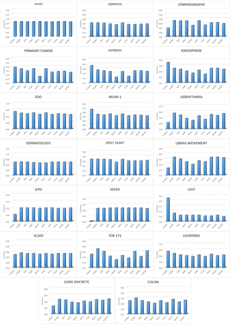
Predicted accuracy levels of all algorithms can be seen in Fig. 3 . E-ADAD has a better performance among most of the datasets (12 in 20) when compared to all of the algorithms presented in (Too & Mirjalili, 2021).

Fig. 3.

Accuracy of Datasets.

In a typical learning prediction model, all data has been divided into three parts, training, validation, and test subsets. This discrimination has some drawbacks, such as test set data in the model and evaluation of the test can hardly be seen on general performance. Grouping data in this way may cause some misplacement. This effect can also be called leakage of data. In addition to this factor, the number of samples for learning or testing can drastically reduce caused after partitioning them. These effects totally can result in worsening the performance of the model.

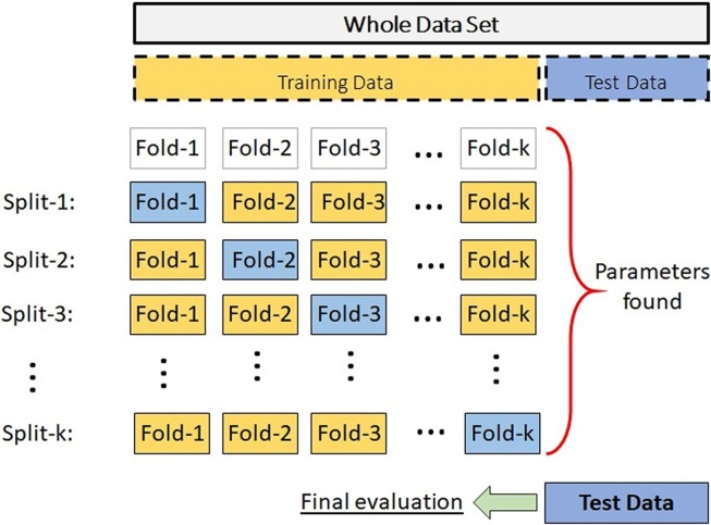
As a solution to this problem, Cross-Validation (CV) has been used in the experiments. CV is in fact a critical technique for avoiding a methodological mistake at the same time. This means that there will be no unseen data up to that time that the model used. In this method, a cross-validation splitting strategy must be determined initially. Then the generator divides or splits the whole data into k equal parts. By default, this k value is 5 in sci-kit library. It means you implement 5-fold cross-validation with the generator.

After splitting the whole data into k “folds”, the model is trained using (k-1) of the folds as training data, and with the last fold, it will be validated. This whole process will be done repeatedly until k times to equally finish all the splits created by the generator in turn. An illustration of k-fold CV is seen in Fig. 4 .

Fig. 4.

k-fold Cross-Validation(CV) Illustration.

Numbers related to the “Learning Curves” and “Fitness Times” of each fold are given in Table 3, Table 4 respectively. The performance of CV is calculated by taking the average of the values of splits computed in turn and all the figures are put together for a clear comparison of the datasets.

Table 3.

Accuracy Learning Curves of the datasets.

No	Dataset	Folds					Average
		#1	#2	#3	#4	#5
1	Glass	0.975	0.975	0.975	0.975	0.975	0.975
2	Hepatitis	0.833	0.833	0.875	0.875	0.917	0.867
3	Lymphography	0.946	0.770	0.838	0.811	0.838	0.840
4	Primary Tumor	0.424	0.424	0.388	0.459	0.388	0.416
5	Soybean	0.744	0.818	0.844	0.883	0.779	0.814
6	Ionosphere	0.943	0.943	0.943	0.955	0.924	0.942
7	Zoo	0.962	1.000	1.000	0.962	0.928	0.970
8	Musk-1	1.000	1.000	1.000	1.000	1.000	1.000
9	Arrhythmia	0.623	0.628	0.637	0.646	0.619	0.631
10	Dermatology	0.982	0.983	0.982	0.966	0.947	0.972
11	SPECT Heart	0.836	0.791	0.866	0.881	0.881	0.851
12	Libras Movement	0.778	0.686	0.789	0.778	0.789	0.764
13	ILPD	0.655	0.710	0.710	0.697	0.710	0.697
14	Seeds	0.906	0.943	0.943	0.962	1.000	0.951
15	LSVT	0.800	0.960	0.920	0.840	0.680	0.840
16	SCADI	0.846	0.846	0.923	0.923	0.712	0.850
17	TOX_171	0.725	0.878	0.813	0.725	0.813	0.791
18	Leukemia	0.929	1.000	1.000	0.929	0.929	0.957
19	Lung discrete	0.929	0.929	0.857	0.843	0.814	0.874
20	Colon	0.917	0.917	0.763	0.877	0.763	0.847

Table 4.

Fitness Times of the datasets.

No	Dataset	Folds					Average
		#1	#2	#3	#4	#5
1	Glass	0.088	0.100	0.113	0.072	0.070	0.089
2	Hepatitis	0.070	0.100	0.071	0.072	0.070	0.077
3	Lymphography	0.059	0.064	0.097	0.110	0.076	0.081
4	Primary	0.125	0.090	0.123	0.106	0.068	0.103
5	Soybean	0.111	0.091	0.082	0.114	0.081	0.096
6	Ionosphere	0.152	0.156	0.147	0.184	0.138	0.155
7	Zoo	0.101	0.084	0.080	0.062	0.070	0.080
8	Musk-1	0.012	0.012	0.022	0.016	0.016	0.016
9	Arrhythmia	0.519	0.512	0.503	0.536	0.434	0.501
10	Dermatology	0.087	0.079	0.096	0.108	0.098	0.094
11	SPECT	0.085	0.100	0.081	0.101	0.063	0.086
12	Libras	0.736	0.492	0.734	0.497	0.677	0.627
13	ILPD	0.086	0.213	0.081	0.091	0.081	0.110
14	Seeds	0.089	0.088	0.092	0.090	0.092	0.090
15	LSVT	0.213	0.301	0.268	0.211	0.210	0.241
16	SCADI	0.016	0.104	0.086	0.058	0.078	0.069
17	TOX_171	6.223	6.520	6.591	6.115	5.770	6.244
18	Leukemia	0.062	0.064	0.091	0.063	0.069	0.070
19	Lung	0.107	0.163	0.109	0.121	0.101	0.120
20	Colon	0.255	0.053	0.019	0.023	0.018	0.074

Then the performance of CV is calculated by taking the average of the values of splits computed in turn. Though this approach seems to need a high computation time, it gives the advantage of getting rid of randomness data leakage. Additionally, you can get rid of the effect of a small number of training or test datasets simultaneously.

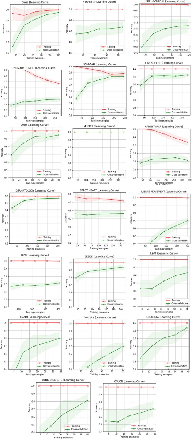
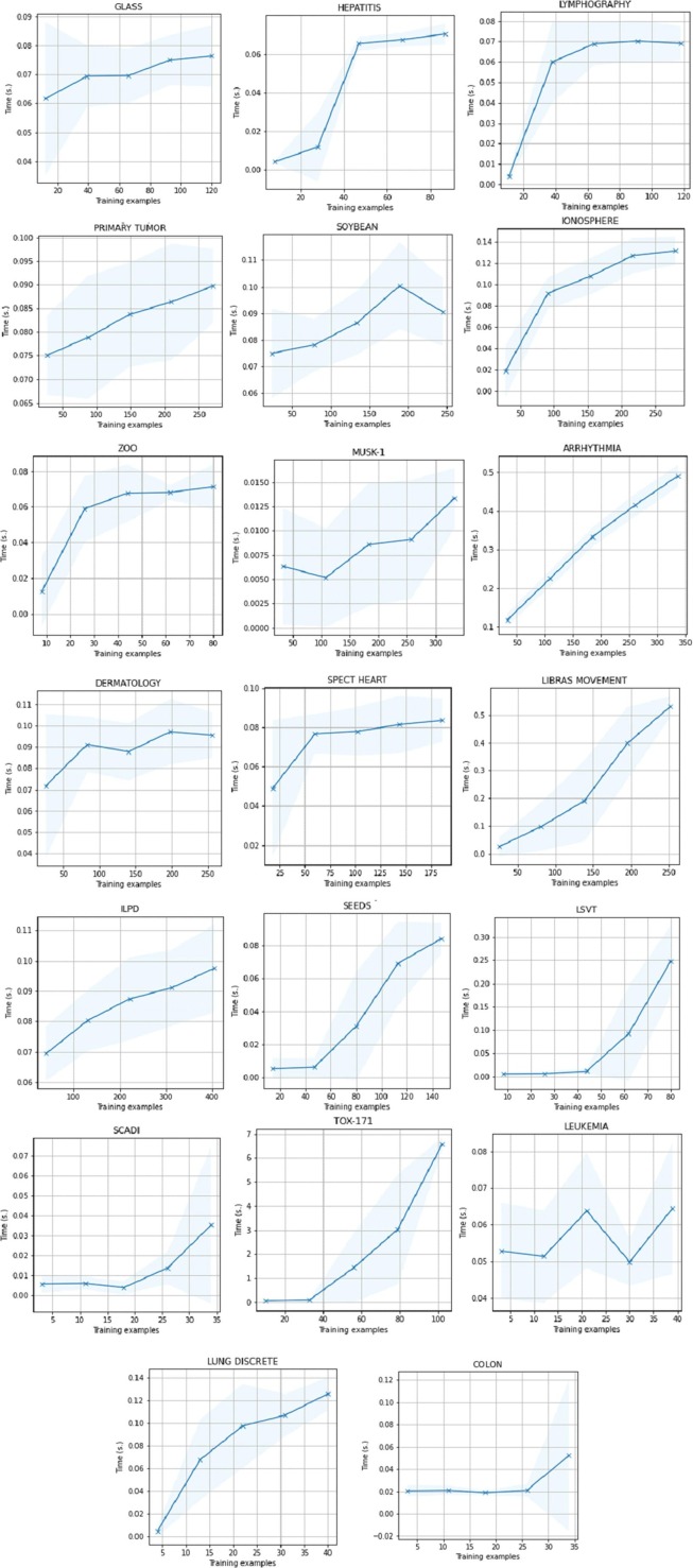
If to see all the methodologies together, “Learning Curves” of Datasets is presented in Fig. 5 , while “Fitness Times” of datasets is in Fig. 6 .

Fig. 5.

Sample Efficiencies of Datasets.

Fig. 6.

Fitness Times of Datasets.

In Fig. 5, learning curve of a Decision Tree classifier is shown as the training set score and the cross-validation scores of the prediction together. This graph is in support of showing accuracy and learning speeds at the same time. These two figures, namely Fig. 5, Fig. 6 are obtained by cross-validator and the whole dataset has been divided by ShuffleSplit function of the sci-kit library. After splitting data into training and test sets, which are 75% and 25% respectively in the study, then the results are automatically evaluated and the results are produced.

High learning curves can easily be noticed. It shows the appropriateness of the model. Then accordingly, a high cross-validation rates is following them. The results of these CV rates are the results of E-ADAD classifier. Then in Fig. 6, the model shows the time how the CV results has been achieved in seconds. It seems extremely fast when compared to its rivals.

Finally, the proposed algorithm has a very fast convergence speed and learning rate, even in the early iterations as clearly seen in Fig. 5, Fig. 6.

4.3. Real dataset comparison

2020 began with a disaster, and the World Health Organization (WHO) announced that Covid-19 became an epidemic. Unfortunately, initial cases were met in China, and the virus rapidly spread over the world. Still, we have many restrictions in our daily life.

In this section, the proposed algorithm is used to solve a real-life problem, namely a Covid-19 patient health prediction dataset. This dataset is the same as in (Too & Mirjalili, 2021), and it can be found on (Atharva-Peshkar) on the Internet.

The description of the dataset is shown in Table 5 . In the dataset, some symptoms are given and accordingly, the death and recovery conditions are given related to given factors due to those 15 features.

Table 5.

The description of Covid-19 Dataset

No	Feature Name	Description
1	id	ID of patient
2	location	The place where patients live
3	country	The country patients belong to
4	gender	The gender of patients
5	age	The ages of patients
6	sym_on	The date patients show the symptoms
7	hosp_vis	The date patients visit hospital
8	vis_wuhan	Whether the patients visited Wuhan, China
9	from_wuhan	Whether the patients come from Wuhan, China
10	symptom1	Name and type of symptoms
11	symptom2	Name and type of symptoms
12	symptom3	Name and type of symptoms
13	symptom4	Name and type of symptoms
14	symptom5	Name and type of symptoms
15	symptom6	Name and type of symptoms

In the whole dataset, there are 1081 instances totally. 1018 instances out of 1081 have the value “0” which denotes alive and the rest 63 instances have the value “1” which denotes dead. In the whole dataset, there are totally 1081 instances. 1018 instances out of 1081 have the value “0” which denotes alive and the rest 63 instances have the value “1” which denotes dead. There are totally 2 classes in the whole dataset. 75% and 25% were used in the study for training and testing sets respectively.

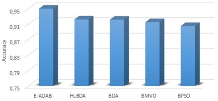
This study is intended to make a comparison with the algorithms in (Too & Mirjalili, 2021) since it is the most recent, state-of-the-art, and published ML algorithm. The proposed algorithm of that study is HLBDA, and additional four other algorithms (HLBDA, BDA, BMVO, and BPSO) have been compared, which are stated there. The parameters pl and gl of HLBDA are declared to be set to 0.7 and 0.85, respectively, and success rates are given in the study. It is told that after updating these two values as stated, HLBDA had a fast convergence speed, which means it gets closer to the final result very quickly. Then it is also claimed that HLBDA had a better success learning rate due to the other mentioned four algorithms.

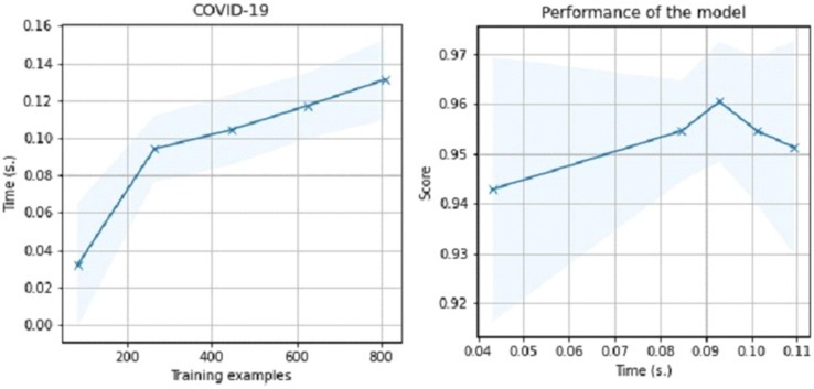
The results are presented in Fig. 7, Fig. 8 . The results of model performance due to the training set and the model is as seen in Fig. 7. Though the proposed algorithm in that study is told to be converged very quickly, E-ADAD trains all training set in 0.14 s and it reaches a better accuracy rate in the period.

Fig. 7.

Performance of the model.

Fig. 8.

Accuracy graph of the algorithms for Covid dataset.

Fig. 8 shows the accuracy rates of all algorithms. E-ADAD has got a 95.33% accuracy rate, and this value is the mean of 10 independent runs. It overcomes HLBDA with 92.21% prediction accuracy being the highest among others in that study.

E-ADAD has the best prediction rate even in a short period. With the help of the “Decision Tree” classifier, E-ADAD has overcome all the other recent and state-of-the-art algorithms.

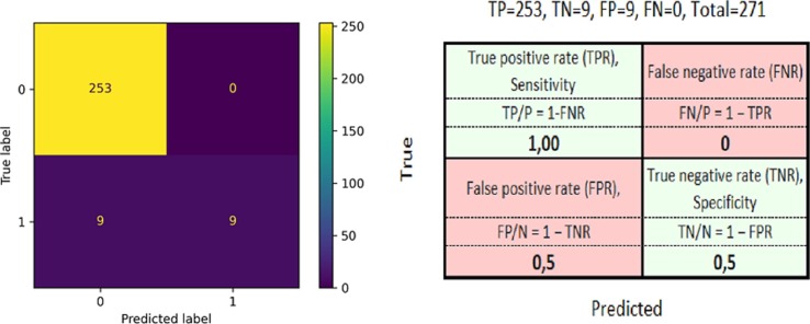
Moreover, two more methods are mentioned for emphasizing the capability of the E-ADAD algorithm. The first one is confusion matrix commonly used for summarizing the performance of a classification algorithm. It is specifically used for the cases if there is a big difference between the classes. A binary data set is used here and in the test dataset, there are 271 instances which are 25% of 1081 total instances. 253 of these are declared as “0”, meaning NOT death, and 18 of these are “1” in the test part as seen in Fig. 9 . Anyway, proportions are being preserved as they are on the whole.

Fig. 9.

Confusion matrix of Covid dataset.

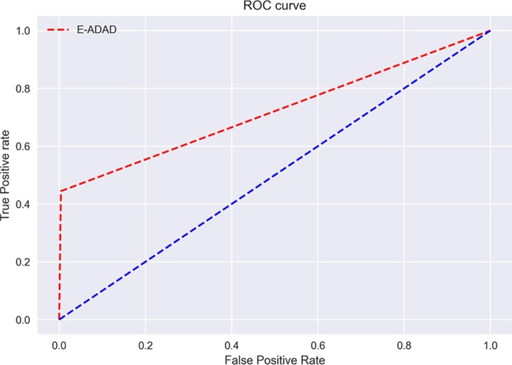
Receiver Operating Characteristic (ROC) curve is also another parameter to evaluate classifier output quality. One characteristic of ROC curves is that the “true positive rate”s are placed on the Y axis, while “false positive rate”s are on the X-axis. In other words, the top left corner of the plot is the “ideal” point - a false positive rate of zero, and a true positive rate of one. However, this point is an extreme, but the closer the better. It implies that a larger Area Under the Curve (AUC) is simply preferable.

The AUC in the proposed algorithm is evaluated as 0.722 and the blue line shows no sign of classification capability or random selectivity while the red line shows the E-ADAD’s performance. This implies a reasonable and remarkable classification has been achieved between the classes of the binary dataset as seen in Fig. 10 .

Fig. 10.

ROC curve of E-ADAD Algorithm.

5. Conclusion and future work

In this study, an Adaptive Boost Algorithm using a Decision Tree estimator is proposed. After making trials, a tuning process is done to a classifier, and a binary classification problem is solved.

AdaBoost is popular and well-known technique in this field. Moreover, it is improved for binary and multi-class classifications. It is seen that the proposed learning model substantially can achieve a good performance both in execution and the average prediction rates. Even for binary classification problems, the algorithm produces way better results than state-of-the-art algorithms. This study is also believed to be used and implemented for other real-life situations during epidemic conditions.

Additionally, for different data and conditions, the E-ADAD algorithm seems to be a good candidate to be benefited. Among its rivals, it seems to predict and achieve in short periods. This is thought to be an outstanding capability and speciality. As a result, E-ADAD achieves the highest accuracy for predicting output classes.

For future studies, E-ADAD can be tuned to get more successful results with multi-class classifications. There is a wide range of research in this field. Especially for regression problems, E-ADAD needs to be searched much for getting far better results. There are many ML fields in new models, and classifiers are proposed and put forward for better results.

Additionally, ensemble algorithms are very promising for proposing new models. Probable newly proposed models with different classifiers can be very beneficial while solving other types of real-life problems. An ensemble algorithm integrated can be useful for especially unsupervised learning and unlabeled data.

References

- Albadr M.A.A., Tiun S., Ayob M., Al-Dhief F.T., Omar K., Hamzah F.A. Optimised genetic algorithm-extreme learning machine approach for automatic covid-19 detection. PloS One. 2020;15(12):e0242899. doi: 10.1371/journal.pone.0242899. [DOI] [PMC free article] [PubMed] [Google Scholar]
- Al-Madi N., Faris H., Mirjalili S. Binary multi-verse optimization algorithm for global optimization and discrete problems. International Journal of Machine Learning and Cybernetics. 2019;10(12):3445–3465. [Google Scholar]
- Api reference. URL https://scikit-learn.org/stable/modules/classes.html.
- Atharva-Peshkar. Atharva-peshkar/covid-19-patient-health-analytics. https://github.com/Atharva-Peshkar/Covid-19-Patient-Health-Analytics.
- Bai Y., Xie J., Wang D., Zhang W., Li C. A manufacturing quality prediction model based on adaboost-lstm with rough knowledge. Computers & Industrial Engineering. 2021;155:107227. [Google Scholar]
- Cao Y., Miao Q.-G., Liu J.-C., Gao L. Advance and prospects of adaboost algorithm. Acta Automatica Sinica. 2014;39(6):745–758. doi: 10.3724/sp.j.1004.2013.00745. [DOI] [Google Scholar]
- Datasets: Feature selection @ asu. https://jundongl.github.io/scikit-feature/datasets.html.
- Deniz A., Kiziloz H.E., Dokeroglu T., Cosar A. Robust multiobjective evolutionary feature subset selection algorithm for binary classification using machine learning techniques. Neurocomputing. 2017;241:128–146. doi: 10.1016/j.neucom.2017.02.033. [DOI] [Google Scholar]
- de Souza R.C.T., de Macedo C.A., dos Santos Coelho L., Pierezan J., Mariani V.C. Binary coyote optimization algorithm for feature selection. Pattern Recognition. 2020;107:107470. [Google Scholar]
- Dokeroglu T., Sevinc E. Evolutionary parallel extreme learning machines for the data classification problem. Computers and Industrial Engineering. 2019;130:237–249. doi: 10.1016/j.cie.2019.02.024. [DOI] [Google Scholar]
- Dokeroglu T., Sevinc E., Kucukyilmaz T., Cosar A. A survey on new generation metaheuristic algorithms. Computers and Industrial Engineering. 2019;137:106040. doi: 10.1016/j.cie.2019.106040. [DOI] [Google Scholar]
- Freund Y. Boosting a weak learning algorithm by majority. Information and Computation. 1995;121(2):256–285. doi: 10.1006/inco.1995.1136. [DOI] [Google Scholar]
- Freund Y., Schapire R.E. A decision-theoretic generalization of on-line learning and an application to boosting. Journal of Computer and System Sciences. 1997;55(1):119–139. doi: 10.1006/jcss.1997.1504. [DOI] [Google Scholar]
- Guz U., Cuendet S., Hakkani-Tur D., Tur G. Multi-view semi-supervised learning for dialog act segmentation of speech. IEEE Transactions on Audio, Speech, and Language Processing. 2010;18(2):320–329. doi: 10.1109/tasl.2009.2028371. [DOI] [Google Scholar]
- Hansen N., Kern S. International Conference on Parallel Problem Solving from Nature. Springer; 2004. Evaluating the cma evolution strategy on multimodal test functions; pp. 282–291. [Google Scholar]
- Hastie T., Rosset S., Zhu J., Zou H. Multi-class adaboost, Statistics and its. Interface. 2009;2(3):349–360. [Google Scholar]
- He Y., Xie H., Wong T.-L., Wang X. A novel binary artificial bee colony algorithm for the set-union knapsack problem. Future Generation Computer Systems. 2018;78:77–86. [Google Scholar]
- Huang G.-B., Zhou H., Ding X., Zhang R. Extreme learning machine for regression and multiclass classification. IEEE Transactions on Systems, Man, and Cybernetics, Part B (Cybernetics) 2012;42(2):513–529. doi: 10.1109/tsmcb.2011.2168604. [DOI] [PubMed] [Google Scholar]
- Jabri, S., Saidallah, M., Alaoui, A. E. B. E., & Fergougui, A. E. (2018). Moving vehicle detection using haar-like, lbp and a machine learning adaboost algorithm. In 2018 IEEE International Conference on Image Processing, Applications and Systems (IPAS). https://doi.org/10.1109/ipas.2018.8708898.
- Karakaya, M. (2017). Sevinc, An efficient genetic algorithm for routing multiple uavs under flight range and service time window constraints.
- Kennedy, J. & Eberhart, R. C. (1997). A discrete binary version of the particle swarm algorithm. In 1997 IEEE International conference on systems, man, and cybernetics. Computational cybernetics and simulation (Vol. 5, pp. 4104–4108). IEEE.
- Khan F., Ahamed J., Kadry S., Ramasamy L.K. Detecting malicious urls using binary classification through adaboost algorithm. International Journal of Electrical and Computer Engineering (IJECE) 2020;10(1):997. doi: 10.11591/ijece.v10i1.pp997-1005. [DOI] [Google Scholar]
- Kiziloz H.E. Classifier ensemble methods in feature selection. Neurocomputing. 2021;419:97–107. doi: 10.1016/j.neucom.2020.07.113. [DOI] [Google Scholar]
- Lai C.-C., Shih T.-P., Ko W.-C., Tang H.-J., Hsueh P.-R. Severe acute respiratory syndrome coronavirus 2 (sars-cov-2) and coronavirus disease-2019 (covid-19): The epidemic and the challenges. International Journal of Antimicrobial Agents. 2020;55(3):105924. doi: 10.1016/j.ijantimicag.2020.105924. [DOI] [PMC free article] [PubMed] [Google Scholar]
- Li J., Kang H., Sun G., Feng T., Li W., Zhang W., Ji B. Ibda: Improved binary dragonfly algorithm with evolutionary population dynamics and adaptive crossover for feature selection. IEEE Access. 2020;8:108032–108051. doi: 10.1109/access.2020.3001204. [DOI] [Google Scholar]
- Lu M. Embedded feature selection accounting for unknown data heterogeneity. Expert Systems with Applications. 2019;119:350–361. [Google Scholar]
- Lu J., Hu H., Bai Y. Generalized radial basis function neural network based on an improved dynamic particle swarm optimization and adaboost algorithm. Neurocomputing. 2015;152:305–315. doi: 10.1016/j.neucom.2014.10.065. [DOI] [Google Scholar]
- Mirjalili S. Dragonfly algorithm: a new meta-heuristic optimization technique for solving single-objective, discrete, and multi-objective problems. Neural Computing and Applications. 2015;27(4):1053–1073. doi: 10.1007/s00521-015-1920-1. [DOI] [Google Scholar]
- Mirjalili S. Dragonfly algorithm: a new meta-heuristic optimization technique for solving single-objective, discrete, and multi-objective problems. Neural Computing and Applications. 2016;27(4):1053–1073. [Google Scholar]
- Priore P., Ponte B., Puente J., Gómez A. Learning-based scheduling of flexible manufacturing systems using ensemble methods. Computers & Industrial Engineering. 2018;126:282–291. [Google Scholar]
- Raileanu L.E., Stoffel K. Theoretical comparison between the gini index and information gain criteria. Annals of Mathematics and Artificial Intelligence. 2004;41(1):77–93. [Google Scholar]
- Sayed G.I., Hassanien A.E., Azar A.T. Feature selection via a novel chaotic crow search algorithm. Neural Computing and Applications. 2019;31(1):171–188. [Google Scholar]
- Schapire R.E. The boosting approach to machine learning: An overview. Nonlinear Estimation and Classification Lecture Notes in Statistics. 2003:149–171. doi: 10.1007/978-0-387-21579-2_9. [DOI] [Google Scholar]
- Seni G., Elder J.F. Ensemble methods in data mining: improving accuracy through combining predictions. Synthesis Lectures on Data Mining and Knowledge Discovery. 2010;2(1):1–126. [Google Scholar]
- Sevinc E. A novel evolutionary algorithm for data classification problem with extreme learning machines. IEEE Access. 2019;7:122419–122427. doi: 10.1109/access.2019.2938271. [DOI] [Google Scholar]
- Sevinç E., Dökeroglu T. A novel hybrid teaching-learning-based optimization algorithm for the classification of data by using extreme learning machines. Turkish Journal Of Electrical Engineering and Computer Sciences. 2019:1523–1533. doi: 10.3906/elk-1802-40. [DOI] [Google Scholar]
- Shhadat I., Hayajneh A., Al-Sharif Z.A. The use of machine learning techniques to advance the detection and classification of unknown malware. Procedia Computer Science. 2020;170:917–922. [Google Scholar]
- Souza E.N.D., Matwin S. Improvements to adaboost dynamic, Advances in Artificial Intelligence. Lecture Notes in Computer Science. 2012:293–298. doi: 10.1007/978-3-642-30353-1_26. [DOI] [Google Scholar]
- Tanabe R., Fukunaga A.S. 2014 IEEE congress on evolutionary computation (CEC) IEEE; 2014. Improving the search performance of shade using linear population size reduction; pp. 1658–1665. [Google Scholar]
- Too J., Mirjalili S. A hyper learning binary dragonfly algorithm for feature selection: A covid-19 case study. Knowledge-Based Systems. 2021;212:106553. doi: 10.1016/j.knosys.2020.106553. [DOI] [Google Scholar]
- Uci machine learning repository: data sets. https://archive.ics.uci.edu/ml/datasets.php.
- Wang F., Liao F., Li Y., Yan X., Chen X. An ensemble learning based multi-objective evolutionary algorithm for the dynamic vehicle routing problem with time windows. Computers & Industrial Engineering. 2021;154:107131. [Google Scholar]
- Who coronavirus (covid-19) dashboard. https://covid19.who.int/.
- Xue Y., Wang N., Yan N., Zhong P., Niu S., Song Y. Robust re-weighted multi-view feature selection. CMC-Computers Materials & Continua. 2019;60(2):741–756. [Google Scholar]
- Zhu Z., Ong Y.-S., Dash M. Wrapper–filter feature selection algorithm using a memetic framework. IEEE Transactions on Systems, Man and Cybernetics, Part B (Cybernetics) 2007;37(1):70–76. doi: 10.1109/tsmcb.2006.883267. [DOI] [PubMed] [Google Scholar]