

Abstract
Cancer can be considered as one of the leading causes of death widely. One of the most effective tools to be able to handle cancer diagnosis, prognosis, and treatment is by using expression profiling technique which is based on microarray gene. For each data point (sample), gene data expression usually receives tens of thousands of genes. As a result, this data is large-scale, high-dimensional, and highly redundant. The classification of gene expression profiles is considered to be a (NP)-Hard problem. Feature (gene) selection is one of the most effective methods to handle this problem. A hybrid cancer classification approach is presented in this paper, and several machine learning techniques were used in the hybrid model: Pearson's correlation coefficient as a correlation-based feature selector and reducer, a Decision Tree classifier that is easy to interpret and does not require a parameter, and Grid Search CV (cross-validation) to optimize the maximum depth hyperparameter. Seven standard microarray cancer datasets are used to evaluate our model. To identify which features are the most informative and relative using the proposed model, various performance measurements are employed, including classification accuracy, specificity, sensitivity, F1-score, and AUC. The suggested strategy greatly decreases the number of genes required for classification, selects the most informative features, and increases classification accuracy, according to the results.
1. Introduction
Cancer can be considered as one of the leading death causes [1], and gene expression profiles derived from microarray data have been identified as promising cancer diagnostic indices [2].
Microarrays are used to measure thousands of genes interactions at the same time and create a cellular function global picture [3, 4].
The classification of microarray data is one of the most common and important applications of functional genomics microarray data which means classifying patients samples to many classes based on their gene expression profiles [5, 48]. In literature, there are many machine learning methods which have been used in the application of microarray data classification [7, 8]. However, the classification process of microarray data is still challenging and difficult due to the small samples numbers and its high dimensionality [9]. Microarray gene expression experiments often generate a lot of features for a small patients number which leads to a high-dimension dataset with a small samples number. Gene expression data is very challenging and complex; genes are correlated with one another directly or indirectly which make classification process a very hard and difficult mission which generally requires using an accurate and powerful feature selection technique.
The main phase in categorization systems is feature selection. To improve classification performance, feature selection-based classification approaches have been investigated. Any statistical technique's [10] success is contingent on the predetermination of independent properties. As a result, identification is kept to a minimum, but the purpose of feature selection is to find the most informative subset of characteristics and/or reduce the number of dimensions.
In order to be able to select an informative genes subset while eliminating/declining redundant or irrelevant genes and to be able to improve the performance of microarray high-dimension data classification, this research study introduces a hybrid feature selection approach, called PCC-DTCV, which combines different methods, Pearson's correlation coefficients (PCC) and Decision Tree (DT) [11] as classification approach and feature selection [12–17] and Grid Search CV which can be employed as an optimization technique [13, 14, 18–20, 42–47], to optimize the tuning parameters of DT (max-depth) to be able to get the optimal feature subset.
In order to evaluate the suggested PCC-DTCV model, 7 popular datasets from the most well-known used microarray datasets for different cancer types are used. The proposed model evaluation was carried out using classification accuracy, k-fold cross-validation, sensitivity, and specificity values.
The proposed method, according to the experimental methods, reduces dimensionality and selects the most important and informative features (genes) and improves the identification of cancer tissues from benign tissues. Furthermore, PCC-DTCV improves the accuracy classification performance.
2. Background and Related Work
Recently, there have been several major research efforts to study the classification and diagnosis of cancer microarray data. As a framework for the study presented in the remainder of the article, we offer an outline of some of this analysis and the applied techniques in Table 1.
Table 1.
Review of previous studies on the feature selection, optimization, and classification methods.
| Author | Datasets | Method | Remark |
|---|---|---|---|
| [29] Shukla and Tripathi (2020) | DLBCL | (JMI) Joint mutual information (mRMR) information gain (IG) | This research introduced modern filter-based gene selection technique for detecting biomarkers from microarray data. |
| [30] Kilicarslan et al. (2020) | Ovarian, leukemia, and Central Nervous system (CNS) | Relief-F of support vector machines (SVM), coevolutionary neural networks (CNN) | This research introduced a hybrid approach based on Relief-F and CNN for cancer diagnosis and classification. |
| [31] Pashaei et al. (2016) | Colon tumor ALL, AML, 4 (CNS) MLL | Binary black hole algorithm (BBHA) and random forest ranking (RFR) | The authors introduced gene selection and classification techniques to microarray data based on RFR and BBHA. |
| [32] Pradana and Aditsania | Breast cancer | Binary particle swarm optimization (BPSO) and Decision Tree C4.5 | This research introduced binary PSO and DT for cancer detection based on microarray data classification. |
| [33] Mantovani et al. | UCI | J48 DTs | They presented induction algorithm and introduced hyperparameter tuning of a Decision Tree induction algorithm. |
| [34] Abbas et al. (2021) | Breast cancer | Whale optimization algorithm (WOA), extremely randomized tree BCD-WERT | This research introduced a novel model for breast cancer detection using WOA optimization based on extremely randomized tree algorithm and efficient features. |
| [35] Reddy et al. | Srivastava, G. (2020) | UCI heart disease | This research presented an adaptive genetic fuzzy logic algorithm and introduced a hybrid GA and a fuzzy logic classifier for heart diagnosis and disease. |
| [36] Qaraad et al. (2020) | Colon cancer, breast cancer, prostate cancer | Elastic NET PSO algorithm | This research introduced parameters optimization of Elastic NET using PSO algorithm for high-dimensional data. |
| [37] El Kafrawy et al. (2020) | De novo acute myeloid leukemia | Recursive feature elimination (RFE), tree-based feature selection (TBFS) | This research introduced multifeature selection with machine learning for de novo acute myeloid leukemia in Egypt. |
| [38] Turgut et al. (2020) | Breast cancer | AdaBoost and Gradient Boosting random forest, logistic regression | This research introduced classification for microarray breast cancer data using machine learning methods. |
3. Preliminaries
3.1. DNA Microarray
One of the main tools employed in molecular biology and genetics to track gene expression is the DNA microarray, which refers to the degree of development of genome-determined protein molecules. Although the protein structure varies from the mRNA measurement gene instead of protein structure, it is a popular method for calculating gene expression, so thousands of proteins would be difficult to analyse, and mRNA sequences [39] are hybridized with their additional DNA or RNA sequences, although proteins do not have these properties. Figure 1 shows experimental microarray steps that include the extraction of mRNA from a cell or tissue. The structure of the DNA microarray matrix is shown in Figure 2, described by N (gene measurement) × M (a sample or condition involved in a specific microarray experiment).
Figure 1.
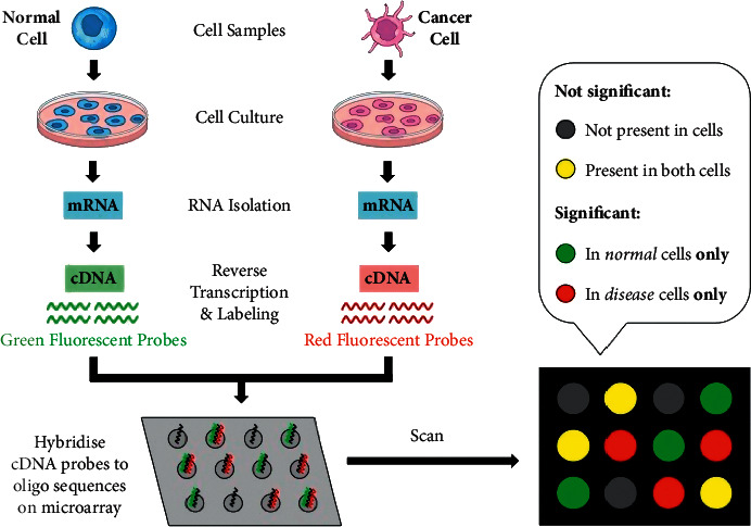
Experiment steps of microarray.
Figure 2.
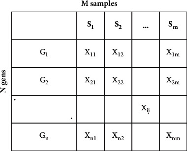
Microarray data matrix structure.
The data on gene expression given by microarray experiments are processed as the broad matrix, where the samples are defined by the columns S{S1,…, Sm} and xij measured the expression strength of the i-th gene (i=1,…, n, and n is the genes number) in the j-th sample (j=1,…, m and m characterize the samples or experimental conditions). The row of genes represents G (gene1,…, genen). In this study, we concentrate on solving two problems: the analysis and understanding of microarray data which have faced several challenges:
High dimensionality and noise
Increasing the accuracy performance taking into consideration interpretations that are biologically significant in gene expression when analysing microarray data
3.2. Decision Tree (DT)
Decision Tree learning can be considered as one of the most practical and commonly used methods for inductive inference.
It is a technique used for approximating discrete-valued functions that can learn disjunctive expressions and is resilient to noisy data [21]. These inductive inference algorithms are among the most common, and they have been successfully employed for a wide range of tasks, from learning up to diagnosis of the medical cases to learn to assess the loan applicants credit risk. Decision Tree learning is a nonbacktracking, one-step lookahead (hill-climbing) quest through the space of all possible Decision Trees using a heuristic. Decision Trees are commonly used in bioinformatics, especially in decision analysis to help identify a type of disease that is more likely to produce a specific symptom. A tree-based classifier was used in our proposed model PCC-DTCV for its basic properties, explicit context, and fast transformation to if-then law. The Decision Tree is a device for decision support which uses a dendritic graph and its potential problems, including unintended incident effects, resource costs, and utility. In bioinformatics, Decision Trees are widely used, especially in decision analysis to help classify a type of disease more likely to achieve a certain symptom. As a descriptive means for manipulating conditional probabilities, the Decision Tree may be used. This works to isolate and conquer [22] methods for creating a Decision Tree. As shown in equations (1)–(5), Entropy controls how a Decision Tree determines to divide the data. It influences how the borders are drawn by a Decision Tree. The Gini (Gini impurity) index measures the degree of probability of a feature that is incorrectly labelled to be randomly selected. The mistakes are in classification. The gain ratio is the parameter of the Decision Tree for measuring output and it is defined as
| (1) |
| (2) |
| (3) |
where n is the number of classes and 0 log_20 = 0 in entropy calculations:
| (4) |
and the function SplitInfo is defined as follows:
| (5) |
where p gives the probability distribution of the data sample and “bit” due to calculating statistics. Equation (5) is used with log function with basis 2. The relation between Entropy, misclassification error, and Gini impurity is seen in Figure 3.
Figure 3.
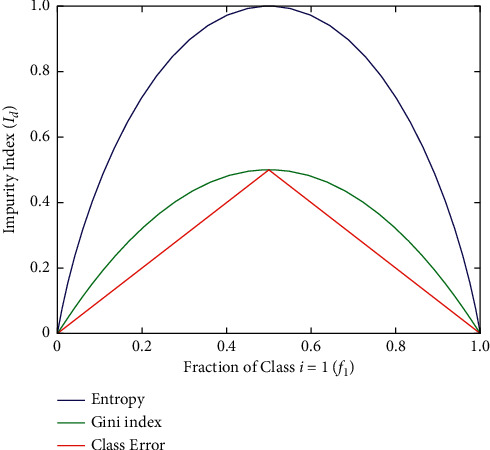
The relation between Gini impurity, Entropy, and misclassification error. [22].
3.3. Correlation Coefficients
The Correlation-based Feature Selection algorithm computes the correlation coefficient using a correlation-based heuristic evaluation function (CFS). It gets over the limitation of univariate filter approaches which do not take into account feature interaction [23, 24]. The process of correlation [25] can be used to measure the relationship between variables (genes). The linear relationship between 2 variables can be described using Pearson's correlation coefficients or correlation coefficients in statistics. The well-known similarity measure between two features is defined as correlation. If two features depend on each other linearly then their coefficient of correlation is ±1. The correlation coefficient is 0 if the features are uncorrelated. For a pair of variables (X, Y), the coefficient of linear correlation r is given by the following equation [26]:
| (6) |
In our model, we used Pearson's correlation coefficient (PCC) as feature selection [38]. This is a mathematical strength measure of a paired data linear relationship. It is defined by r and is limited as follows:
, in which positive values mean that the linear correlation is positive, negative values imply that the linear correlation is negative, zero value means there is a nonlinear correlation, and the closer the value is to −1 or 1, the stronger the linear correlation exists.
The proposed model used Pearson's correlation to calculate the correlation between the features. Also using symmetric uncertainty measures, the class feature is calculated. If the value is higher than the threshold value (0.5), then the feature will be chosen. The selection ends when the number of features equals n log n. According to the decreasing order, each selected feature is ranked. To remove the redundant feature, the feature-feature correlation is done. Threshold values (0.4, 0.5, and 0.6) were used and their results were compared with the Decision Tree before and after the optimization of its maximum depth (max-depth).
3.4. Grid Search Cross-Validation
A Grid Search is a parameter tuning method which builds and evaluates a model methodically for each algorithm parameters combination specified in a grid. The well-known terms that should be addressed while using Grid Search CV are discussed as follows [27].
Estimator. This term is used in order to implement the estimator interface in scikit-learn. This parameter receives the classifier to be trained [28].
Parameter Grid. It is a Python key-value dictionary with pairs of parameter names and parameter settings. All combinations of these parameters are tested to ensure the highest level of accuracy.
Cross-Validation. This determines the strategy for cross-validation splitting. Cross-validation is a technique to resample available data to evaluate machine learning models. The main goal of this is to evaluate the performance of machine learning models on previously unseen data. The main advantage of using this is that it produces less biased or optimistic results compared to a simple train-test split. The way it works is that it first shuffles the dataset randomly. The entire dataset is then divided into k groups. Each group is used as test data, while the others are used as training data. The evaluation band related to each group is saved to be summarized at the end to be able to check the performance of the model. Importantly, each sample appears once in the testing data and is used to train k − 1 times. Figure 4 explains the Grid Search cross-validation process in detail.
During the training step, hyperparameters that are optimizer variables are executed to get optimal average values after several trial-and-error processes. The tree maximum depth (max-depth) is the most critical hyperparameter that influences the difficulty of the Decision Tree model [6], whereas the maximum depth is the length of the longest distance from the tree root to a node. The root node is 0.0 in depth. The higher overall depth value induces overfitting, and the lower value results in underfitting. In the proposed hybrid model PCC-DTCV, Grid Search cross-validation is used to overcome the overfitting constraint with the regular Grid Search. To obtain better parameters, Grid Search cross-validation is used to optimize the tree maximum depth hyperparameter to get optimal hyperparameter value.
Figure 4.
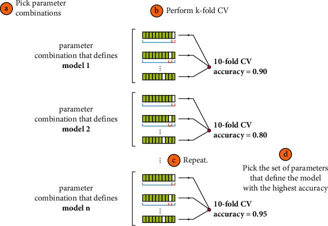
Working of Grid Search cross-validation [26].
4. Proposed Model PCC-DTCV
The proposed hybrid model PCC-DTCV for classifying and diagnosing cancer microarray data (as shown in Figure 5) will be clarified in detail. Key model phases are as follows: (1) The datasets (cancer microarray) are preprocessed. This stage is essential to (a) avoid features in wide digital ranges dominating fewer ranges, (b) avoid numeric complexities through calculation, and (c) adjust each feature to the range [0,1]. (2) PCC is applied for finding the association between the continuous features and the class feature, evaluation to genes is based on how it is related to targeting the features that have a high correlation with the target class having a correlation value near to 1, and the genes with the correlation coefficient ≥0.5 are removed and the output subsets are informative and important genes (features). (3) The sample data output subset is the partition used to train data to match the model and test data used to validate the model as soon as a model is fully trained (trained DT). (4) Grid Search CV with 10-fold cross-validation is used to obtain the optimal parameters (max-depth) of the tree on the training set. (5) Model accuracy is evaluated, using 10-fold cross-validation, and our dataset is 10-fold split, using train split to train the classifier, and prediction quality on unseen data is estimated (test split). The confusion matrix is measured for test split. The AUC, specificity, and sensitivity in addition to accuracy are computed. (6) If the termination conditions are not met, the process from three to six is repeated until the termination criteria are satisfied. If the termination is fulfilled (max folds, number = 10), the result will be a subset of optimal genes (features) with the most important and informative genes.
Figure 5.
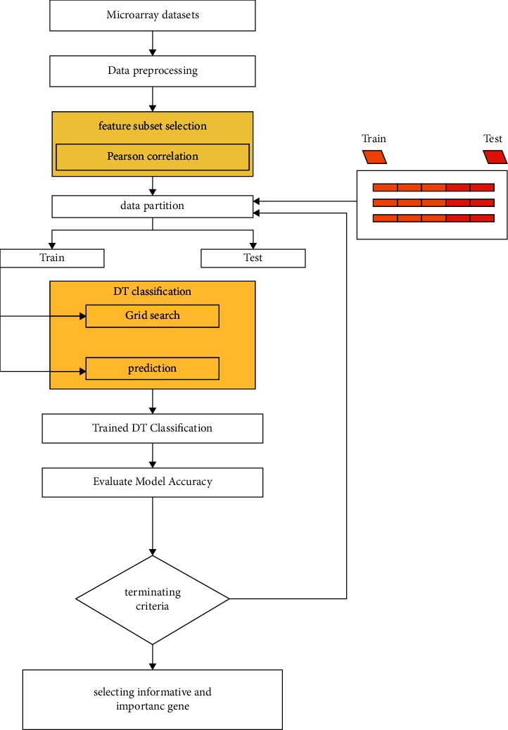
Proposed model (PCC-DTCV).
5. Results and Discussion
In the following section, the findings of numerous studies that have been performed to determine the efficacy of the proposed hybrid model PCC-DTCV are discussed. A PC with the following properties is the platform used to test the proposed model: RAM 4 GB and 32-bit OS (Windows 7), Intel(R) Core (TM) i5-7500CPU, as well as frameworks such as Pandas, NumPy, Keras, SciPy, and Matplotlib and the Python programming language. The datasets for human cancer research included the following: breast cancer, prostate, colon tumor, lung cancer, and leukemia were applied to 7 different microarray datasets with a limited sample and high-dimensional and binary class. Also, all datasets have two types, and Table 2 lists the definitions of all datasets.
Table 2.
Characterization of the dataset.
| Disease | Dataset | No. of samples | No. of features |
|---|---|---|---|
| Prostate cancer | D1, Singh [21] | 102 | 12600 |
| Lung cancer | D2, Gordon [22] | 181 | 12533 |
| Breast cancer | D3, Chowdary [23] | 104 | 22283 |
| Colon cancer | D4, Alon [24] | 62 | 2000 |
| Breast cancer | D5, Chin [25] | 118 | 22215 |
| Breast cancer | D6, West [26] | 49 | 7129 |
| Leukemia | D7, Golub [27] | 72 | 7129 |
In all studies, 10-fold cross-validation techniques were applied. The data were randomly divided into 10 different subsets (with the same size in 10-fold cross-validation), and the experiment was conducted 10 times. One subset was used as a test set for each run, and one was used as a validation set, and the other sets were used as a training set (Figure 5). To obtain a single estimate, the mean of the k results from the folds can then be determined. To approximate the model, 10-fold cross-validation was used in our experiments, and the results obtained are illustrated in the form of mean ± standard deviation. Also, in both analyses, the number of iterations was 50. The value of the tree (max-depth) hyperparameter is [3, 30]. Our evaluation included the four following measurements:
Accuracy (ACC): it is the most used evaluation standard for the proportion of correctly predicted pairs, but using it alone is usually insufficient. Accuracy (ACC)=((TP+TN)/(TP+TN+FP+FN)).
Sensitivity (Sen.): a diseased person is likely to be recognized as diseased through the test. S=(TP/(TP+TN)), where TN is the true negatives number and TP is the true positives number.
Specificity (Spec.): the likelihood is that a person without the illness is defined by the test as nondiseased (or healthy). It is described as TRN=(TN/(TP+TN)), where FP implies the number of false positives and TN is the number of true negatives.
The AUC shows the area under the receiver operating characteristics (ROC) curve, and it is calculated as AUC=(1+TPR − FPR)/2.
TP is true positive, FP is false positive, TN is true negative, and FN is false negative. Based on the confusion matrix, we evaluated the performance of the proposed method and rival gene selection. To assess the output of our model, a statistical test method called Chi-Square test [21] is used to check how well the observed values for a given distribution fit the distribution when the variables are independent.
6. Experimental Results
The experimental results are discussed in this section to validate the performance of the our model PCC-DTCV. The classification accuracy performance and the selected feature (genes) numbers of the PCC-DTCV method with PCC (0.4, 0.5, and 0.6) for all microarray datasets, respectively, are summarized in Tables 3–8 and Figures 6–9. The statistical model is described in Table 9. Six different performance metrics were chosen for result estimation: AUC, ACC, specificity, sensitivity, recall, and F1-score [10, 22]. To reduce the high dimensionality, improve the classification performance of the problem at hand, and select the most informative genes, we run PCC-DTCV using all datasets and get the informative selected features (genes) number. It can be noted that PCC-DTCV gives the genes (features) ordered list according to the highest correlation informative, importance, and relevant genes. It is obvious that PCC-DTCV achieves the highest level of dimensional reduction by choosing smallest number of informative genes and the biggest dimensional dataset is Chowdary for breast cancer with 22283 features (genes) and 104 samples, as seen in Tables 3 and 4. The highly correlated subset selected genes with the target class by the PCC-DTCV with PPC ≥= 0.4 are 410 features (genes) from 22283. PCC-DTCV compared the performance of DT classifier without any optimization method and optimized DT as given in Tables 3 and 4, respectively, as well as the accuracy of the highest-dimensional dataset with PPC ≥= 0.4 with optimized DT classifier and DT classifier. With accuracy of (0.92 ± 0.09), the optimized DT classifier shows better accuracy than DT classifier with accuracy of (0.90 ± 0.09).
Table 3.
PCC-DTCV model with DT and PPC ≥0.4.
| Dataset | Features | Selected features | PCC-DTCV model with DT and PPC ≥0.5 | |||||||
|---|---|---|---|---|---|---|---|---|---|---|
| Accuracy | AUC | Sensitivity | Specificity | Recall | F1-score | |||||
| 0 | 1 | 0 | 1 | |||||||
| Singh | 12600 | 299 | 0.77 ± 0.16 | 0.78 ± 0.16 | 0.78 ± 0.19 | 0.77 ± 0.20 | 0.80 | 0.79 | 0.79 | 0.80 |
| Gordon | 12533 | 743 | 0.93 ± 0.06 | 0.88 ± 0.11 | 0.97 ± 0.06 | 0.79 ± 0.24 | 0.95 | 0.71 | 0.95 | 0.73 |
| Chowdary | 22283 | 410 | 0.90 ± 0.09 | 0.89 ± 0.08 | 0.90 ± 0.15 | 0.88 ± 0.12 | 0.94 | 0.88 | 0.93 | 0.89 |
| Alon | 2000 | 61 | 0.79 ± 0.20 | 0.075 ± 0.22 | 0.62 ± 0.37 | 0.88 ± 0.20 | 0.64 | 0.82 | 0.65 | 0.81 |
| Chin | 22215 | 1211 | 0.81 ± 0.12 | 0.80 ± 0.11 | 0.78 ± 0.13 | 0.82 ± 0.17 | 0.79 | 0.85 | 0.77 | 0.86 |
| West | 7129 | 28 | 0.83 ± 0.15 | 0.84 ± 0.16 | 0.82 ± 0.23 | 0.87 ± 0.16 | 0.84 | 0.83 | 0.84 | 0.83 |
| Golub | 7129 | 465 | 0.89 ± 0.11 | 0.87 ± 0.13 | 0.93 ± 0.10 | 0.80 ± 0.21 | 0.89 | 0.76 | 0.88 | 0.78 |
Table 4.
PCC-DTCV model with optimized DT and PPC ≥0.4.
| Dataset | Features | Selected features | PCC-DTCV model with optimized DT and PPC ≥0.5 | |||||||
|---|---|---|---|---|---|---|---|---|---|---|
| Accuracy | AUC | Sensitivity | Specificity | Recall | F1-score | |||||
| 0 | 1 | 0 | 1 | |||||||
| Singh | 12600 | 299 | 0.76 ± 0.12 | 0.76 ± 0.12 | 0.74 ± 0.16 | 0.78 ± 0.21 | 0.80 | 0.81 | 0.80 | 0.81 |
| Gordon | 12533 | 743 | 0.93 ± 0.05 | 0.87 ± 0.11 | 0.97 ± 0.04 | 0.76 ± 0.23 | 0.97 | 0.84 | 0.97 | 0.84 |
| Chowdary | 22283 | 410 | 0.92 ± 0.09 | 0.92 ± 0.09 | 0.94 ± 0.12 | 0.90 ± 0.12 | 0.94 | 0.88 | 0.93 | 0.83 |
| Alon | 2000 | 61 | 0.82 ± 0.13 | 0.80 ± 0.14 | 0.73 ± 0.23 | 0.88 ± 0.17 | 0.73 | 0.82 | 0.71 | 0.84 |
| Chin | 22215 | 1211 | 0.79 ± 0.09 | 0.78 ± 0.10 | 0.74 ± 0.17 | 0.81 ± 0.12 | 0.72 | 0.85 | 0.73 | 0.85 |
| West | 7129 | 28 | 0.86 ± 0.13 | 0.87 ± 0.13 | 0.87 ± 0.21 | 0.87 ± 0.16 | 0.84 | 0.83 | 0.84 | 0.83 |
| Golub | 7129 | 465 | 0.86 ± 0.09 | 0.83 ± 0.12 | 0.92 ± 0.10 | 0.75 ± 0.21 | 0.94 | 0.80 | 0.92 | 0.83 |
Table 5.
PCC-DTCV model with DT and PPC ≥0.5.
| Dataset | Features | Selected features | PCC-DTCV model with optimized DT and PPC ≥0.5 | |||||||
|---|---|---|---|---|---|---|---|---|---|---|
| Accuracy | AUC | Sensitivity | Specificity | Recall | F1-score | |||||
| 0 | 1 | 0 | 1 | |||||||
| Singh | 12600 | 58 | 0.82 ± 0.11 | 0.82 ± 0.10 | 0.88 ± 0.13 | 0.77 ± 0.20 | 0.88 | 0.77 | 0.83 | 0.82 |
| Gordon | 12533 | 274 | 0.94 ± 0.05 | 0.88 ± 0.11 | 0.97 ± 0.05 | 0.79 ± 0.24 | 0.97 | 0.81 | 0.97 | 0.83 |
| Chowdary | 22283 | 39 | 0.91 ± 0.15 | 0.90 ± 0.15 | 0.94 ± 0.12 | 0.86 ± 0.19 | 0.95 | 0.90 | 0.94 | 0.92 |
| Alon | 2000 | 9 | 0.73 ± 0.18 | 0.70 ± 0.17 | 0.63 ± 0.24 | 0.78 ± 0.21 | 0.59 | 0.80 | 0.60 | 0.79 |
| Chin | 22215 | 305 | 0.81 ± 0.09 | 0.80 ± 0.08 | 0.75 ± 0.10 | 0.85 ± 0.14 | 0.72 | 0.85 | 0.73 | 0.85 |
| West | 7129 | 5 | 0.90 ± 0.13 | 0.91 ± 0.13 | 0.92 ± 0.17 | 0.90 ± 0.15 | 0.92 | 0.88 | 0.83 | 0.82 |
| Golub | 7129 | 133 | 0.87 ± 0.08 | 0.85 ± 0.10 | 0.94 ± 0.09 | 0.77 ± 0.20 | 0.91 | 0.80 | 0.91 | 0.82 |
Table 6.
PCC-DTCV model with optimized DT and PPC ≥0.5.
| Dataset | Features | Selected features | PCC-DTCV model with optimized DT and PPC ≥0.5 | |||||||
|---|---|---|---|---|---|---|---|---|---|---|
| Accuracy | AUC | Sensitivity | Specificity | Recall | F1-score | |||||
| 0 | 1 | 0 | 1 | |||||||
| Singh | 12600 | 58 | 0.78 ± 0.15 | 0.78 ± 0.15 | 0.78 ± 0.19 | 0.78 ± 0.23 | 0.78 | 0.83 | 0.80 | 0.81 |
| Gordon | 12533 | 274 | 0.94 ± 0.04 | 0.90 ± 0.08 | 0.97 ± 0.04 | 0.84 ± 0.16 | 0.95 | 0.77 | 0.95 | 0.77 |
| Chowdary | 22283 | 39 | 0.94 ± 0.08 | 0.94 ± 0.08 | 0.95 ± 0.09 | 0.93 ± 0.11 | 0.95 | 0.90 | 0.94 | 0.92 |
| Alon | 2000 | 9 | 0.78 ± 0.19 | 0.75 ± 0.19 | 0.68 ± 0.26 | 0.82 ± 0.23 | 0.68 | 0.80 | 0.67 | 0.81 |
| Chin | 22215 | 305 | 0.82 ± 0.09 | 0.80 ± 0.09 | 0.77 ± 0.15 | 0.84 ± 0.12 | 0.74 | 0.85 | 0.74 | 0.85 |
| West | 7129 | 5 | 0.83 ± 0.18 | 0.83 ± 0.18 | 0.80 ± 0.24 | 0.87 ± 0.16 | 0.84 | 0.83 | 0.84 | 0.83 |
| Golub | 7129 | 133 | 0.89 ± 0.06 | 0.89 ± 0.07 | 0.92 ± 0.10 | 0.85 ± 0.19 | 0.87 | 0.76 | 0.87 | 0.76 |
Table 7.
PCC-DTCV model with DT and PPC ≥0.5.
| Dataset | Features | Selected features | PCC-DTCV model with optimized DT and PPC ≥0.5 | |||||||
|---|---|---|---|---|---|---|---|---|---|---|
| Accuracy | AUC | Sensitivity | Specificity | Recall | F1-score | |||||
| 0 | 1 | 0 | 1 | |||||||
| Singh | 12600 | 10 | 0.90 ± 0.08 | 0.90 ± 0.08 | 0.90 ± 0.10 | 0.90 ± 0.10 | 0.90 | 0.88 | 0.89 | 0.89 |
| Gordon | 12533 | 98 | 0.95 ± 0.05 | 0.89 ± 0.11 | 0.98 ± 0.04 | 0.81 ± 0.22 | 0.99 | 0.74 | 0.97 | 0.84 |
| Chowdary | 22283 | 5 | 0.96 ± 0.06 | 0.96 ± 0.06 | 0.97 ± 0.06 | 0.96 ± 0.12 | 0.95 | 0.93 | 0.95 | 0.93 |
| Alon | 2000 | 1 | 0.72 ± 0.18 | 0.71 ± 0.19 | 0.67 ± 0.32 | 0.75 ± 0.22 | 0.68 | 0.75 | 0.64 | 0.78 |
| Chin | 22215 | 54 | 0.85 ± 0.07 | 0.84 ± 0.08 | 0.82 ± 0.17 | 0.87 ± 0.11 | 0.72 | 0.88 | 0.75 | 0.86 |
| West | 7129 | 2 | 0.82 ± 0.19 | 0.82 ± 0.21 | 0.87 ± 0.32 | 0.85 ± 0.19 | 0.80 | 0.83 | 0.82 | 0.82 |
| Golub | 7129 | 36 | 0.85 ± 0.10 | 0.82 ± 0.12 | 0.89 ± 0.11 | 0.75 ± 0.21 | 0.94 | 0.80 | 0.92 | 0.83 |
Table 8.
PCC-DTCV model with optimized DT and PPC ≥ 0.6.
| Dataset | Features | Selected features | PCC-DTCV model with optimized DT and PPC ≥0.5 | |||||||
|---|---|---|---|---|---|---|---|---|---|---|
| Accuracy | AUC | Sensitivity | Specificity | Recall | F1-score | |||||
| 0 | 1 | 0 | 1 | |||||||
| Singh | 12600 | 10 | 0.89 ± 0.05 | 0.89 ± 0.05 | 0.88 ± 0.10 | 0.90 ± 0.13 | 0.88 | 0.94 | 0.91 | 0.92 |
| Gordon | 12533 | 98 | 0.95 ± 0.04 | 0.87 ± 0.11 | 0.99 ± 0.03 | 0.75 ± 0.23 | 0.99 | 0.77 | 0.97 | 0.84 |
| Chowdary | 22283 | 5 | 0.93 ± 0.06 | 0.93 ± 0.07 | 0.95 ± 0.07 | 0.91 ± 0.14 | 0.97 | 0.90 | 0.95 | 0.93 |
| Alon | 2000 | 1 | 0.79 ± 0.18 | 0.76 ± 0.17 | 0.67 ± 0.22 | 0.85 ± 0.25 | 0.64 | 0.88 | 0.68 | 0.84 |
| Chin | 22215 | 54 | 0.84 ± 0.11 | 0.83 ± 0.12 | 0.78 ± 0.20 | 0.88 ± 0.09 | 0.79 | 0.83 | 0.76 | 0.85 |
| West | 7129 | 2 | 0.83 ± 0.15 | 0.83 ± 0.17 | 0.78 ± 0.32 | 0.88 ± 0.18 | 0.80 | 0.83 | 0.82 | 0.82 |
| Golub | 7129 | 36 | 0.90 ± 0.09 | 0.88 ± 0.12 | 0.96 ± 0.08 | 0.80 ± 0.21 | 0.91 | 0.80 | 0.91 | 0.80 |
Figure 6.
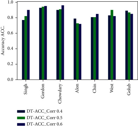
Accuracy obtained for PCC-DTCV model using the DT classifier with PPC ≥0.4, 0.5, and 0.6 for all datasets.
Figure 7.
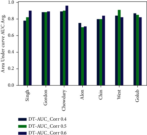
AUC obtained for PCC-DTCV model using the DT classifier with PPC ≥0.4, 0.5, and 0.6 for all datasets.
Figure 8.
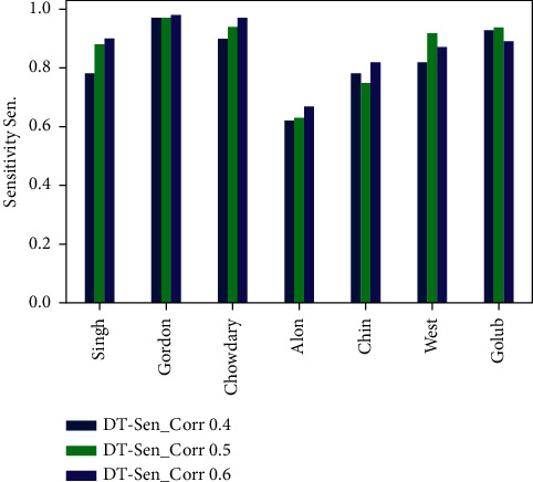
Sensitivity obtained for PCC-DTCV model using the DT classifier with PPC ≥0.4, 0.5, and 0.6 for all datasets.
Figure 9.
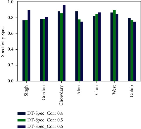
Specificity obtained for PCC-DTCV model using the DT classifier with PPC ≥0.4, 0.5, and 6 for all datasets.
Table 9.
Tests of normality.
| Kolmogorov–Smirnova | Shapiro−Wilk | ||||
|---|---|---|---|---|---|
| PCR | Statistic | Sig. | Statistic | ||
| Spec. DT OPT | ≥0.4 | 0.158 | 0.200∗ | 0.983 | 0.971 |
| ≥0.5 | 0.166 | 0.200∗ | 0.943 | 0.668 | |
| ≥0.6 | 0.257 | 0.178 | 0.940 | 0.639 | |
|
| |||||
| AUC DT OPT | ≥0.4 | 0.161 | 0.200∗ | 0.981 | 0.965 |
| ≥0.5 | 0.190 | 0.200∗ | 0.956 | 0.190 | |
| ≥0.6 | 0.205 | 0.200∗ | 0.892 | 0.285 | |
|
| |||||
| Sen. DT OPT | ≥0.4 | 0.137 | 0.200∗ | 0.962 | 0.832 |
| ≥0.5 | 0.163 | 0.200∗ | 0.926 | 0.517 | |
| ≥0.6 | 0.245 | 0.200∗ | 0.884 | 0.245 | |
|
| |||||
| Sen. DT | ≥0.4 | 0.205 | 0.200∗ | 0.871 | 0.189 |
| ≥0.5 | 0.241 | 0.200∗ | 0.873 | 0.197 | |
| ≥0.6 | 0.275 | 0.117 | 0.905 | 0.364 | |
|
| |||||
| Spec. DT | ≥0.4 | 0.284 | 0.093 | 0.836 | 0.090 |
| ≥0.5 | 0.169 | 0.200∗ | 0.956 | 0.785 | |
| ≥0.6 | 0.188 | 0.200∗ | 0.911 | 0.403 | |
|
| |||||
| AUC DT | ≥0.4 | 0.204 | 0.200∗ | 0.948 | 0.714 |
| ≥0.5 | 0.243 | 0.200∗ | 0.900 | 0.334 | |
| ≥0.6 | 0.233 | 0.200∗ | 0.933 | 0.580 | |
∗ This is a lower bound of the true significance. aLilliefors significance correction.
Tables 5 and 6 show that the number of selected (features) genes with PPC ≥0.5 is lower than the number of selected (features) genes with PPC ≥0.4 for all datasets; it means that the PCC-DTCV achieved higher-dimensional reduction with PPC ≥0.5 than with PPC ≥0.4. In terms of ACC, AUC, sensitivity, and specificity, the PCC-DTCV achieved higher results compared to those achieved with PPC ≥0.4 with both optimized DT classifier and DT classifier; for example, the number of selected (features) genes of Gordon dataset for lung cancer is 274 compared with 743 for PPC ≥0.4, in addition to the values of 94%, 88%, 97%, and 79% for terms ACC, AUC, sensitivity, and specificity with DT classifier and 94%, 90%, 97%, and 87% with optimized DT classifier. From Tables 7 and 8, we can see that the PCC-DTCV with PPC ≥0.6 has the best ACC, AUC, sensitivity, specificity, recall, and F1-score compared to PPC ≥0.4 and 0.5, which means that the classification performance of PCC-DTCV is best with PPC ≥0.6 and the selected genes (features) are the most relevant, important, and informative genes.
Figures 6–9 represent the classification performance obtained using PPC ≥0.4, 0.5, and 0.6 and DT classifier with the PCC-DTCV model for prostate cancer, colon cancer, leukemia, lung cancer, and breast cancer datasets. From Figure 6, the achieved results show that the suggested PCC-DTCV model gives better accuracy for breast cancer, lung cancer, and leukemia datasets and can obtain the highest accuracy with PPC ≥0.6 in the Chowdary dataset for breast cancer, 96%. From Figure 7, the AUC metric obtains more than 90% for both Chowdary and Singh datasets and more than 80% for all datasets except Alon dataset for colon cancer, obtaining 71% for PPC ≥0.6. From Figure 8, the sensitivity metric obtains more than 90 with Gordon, Chowdary, and Golub datasets for lung cancer, breast cancer, and Leukemia, respectively, with PPC ≥0.4, 0.5, and 0.6. Specificity metric shown in Figure 9 achieves 96% for Chowdary dataset with PPC ≥0.6.
Figures 10–13 represent the classification performance obtained using optimized DT classifier and PPC with PCC-DTCV model for prostate cancer, colon cancer, leukemia, lung cancer, and breast cancer datasets. In Figure 10, accuracy metric can obtain more than 90% for Gordon, Chowdary, and Golub datasets for lung cancer, breast cancer, and leukemia, respectively, with PPC ≥0.6. From Figure 11, the AUC metric obtains more than 80% for all datasets except Alon dataset for colon cancer, obtaining 76% for PPC ≥0.6. From Figure 12, the sensitivity metric obtains more than 90% with Gordon, Chowdary, and Golub datasets for lung cancer, breast cancer, and leukemia, respectively, with PPC ≥0.4, 0.5, and 0.6. Specificity metric shown in Figure 13 obtains more than 80% for all datasets with PPC ≥ 0.6. Finally, the proposed model gives the best classification performance with PPC ≥0.6 for both optimized DT classifier and DT classifier and the selected features (genes) have minimum redundancy and are maximally relevant and informative with high correlation with target class.
Figure 10.
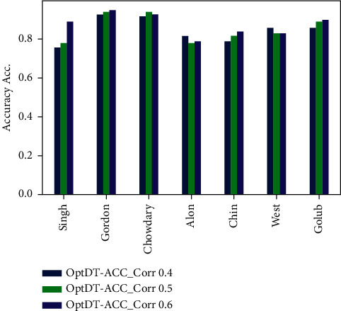
Accuracy obtained for PCC-DTCV model using the DT classifier with PPC ≥0.4, 0.5, and 0.6 for all datasets.
Figure 11.
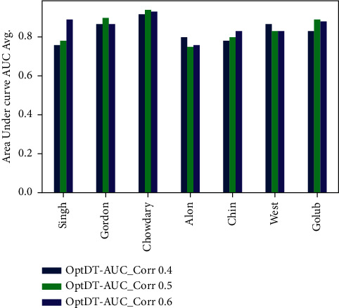
AUC obtained for PCC-DTCV model using the DT classifier with PPC ≥0.4, 0.5, and 0.6 for all datasets.
Figure 12.
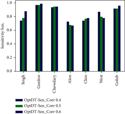
Sensitivity obtained for PCC-DTCV model using the optimized DT classifier with PPC ≥0.4, 0.5, and 0.6 for all datasets.
Figure 13.
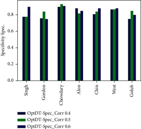
Specificity obtained for PCC-DTCV model using the optimized DT classifier with PPC ≥0.4, 0.5, and 0.6 for all datasets.
These results clarify that the proposed models follow a normal distribution as the value in both Kolmogorov–Smirnov and Shapiro–Wilk Sig. 0.02 ≥ .05 shown in Table 9. The first condition is fulfilled by following a normal distribution. The second condition is that there are no outliers and anomalies, as well as applying regression analysis to use the Manhattan distance method, which calculates the outlier values. In addition, the emergence of a new variable and the largest value in Manhattan distance is compared and it is less valuable than the number of existing variables using the Chi-Square. The value of Manhattan distance = 18.466 compared to using the Chi-Square. The critical value of the Chi-Square distribution will be applied at df = 6 and the p value of 0.001 is found to be at 0.999 confidence interval and uncertainty interval 0.001. If the value of 22.46 is greater than 18.466, then it is assumed that there are no multiple-choice outliers. Sig = .0155, which is greater than 0.0001. It is a fulfilled condition and it means that the homogeneity condition variance exists and is fulfilled by a choice of Finney greater than 0.5. This indicates that the variance of the dependent variables is equal.
7. Conclusions
This paper presents a PCC-DTCV model for cancer diagnosis and classification. PCC-DTCV optimizes the tuning parameter (max-depth) of the DT classifier using Grid Search and Pearson's correlation used as a gene (feature) selection method. The proposed model was effective in identifying an optimal or near-optimal subset of informative and important genes and yielded high classification results. Several experiments were carried out to evaluate the proposed PCC-DTCV model for selecting the most informative genes to improve the performance classification of cancer microarray data. In addition to reducing the dimensionality of microarray data, the result demonstrates the model's effective performance in selecting the most informative genes with high importance. The results showed that PCC-DTCV provides the best fit for cancer type prediction in terms of specificity, AUC, sensitivity, and accuracy. In future work, for Decision Tree optimization, we anticipate using ski driver and other algorithms.
Acknowledgments
This research was supported by the Researchers Supporting Project number (RSP-2021/244), King Saud University, Riyadh, Saudi Arabia.
Contributor Information
Hanaa Fathi, Email: hanaa_4_ever@yahoo.com.
Abdu Gumaei, Email: abdugumaei@taiz.edu.ye.
Data Availability
The data used to support the findings of this study are available from the corresponding author upon request.
Conflicts of Interest
The authors declare that they have no conflicts of interest.
References
- 1.Siegel R. L., Miller K. D., Fuchs H. E., Jemal A. Cancer statistics, 2021. CA: A Cancer Journal for Clinicians . 2021;71(1):7–33. doi: 10.3322/caac.21654. [DOI] [PubMed] [Google Scholar]
- 2.Perez-Diez A., Morgun A., Shulzhenko N. Microarrays for cancer diagnosis and classification. Advances in Experimental Medicine and Biology . 2007;593:74–85. doi: 10.1007/978-0-387-39978-2_8. [DOI] [PubMed] [Google Scholar]
- 3.Pang H., George S. L., Hui K., Tong T. Gene selection using iterative feature elimination random forests for survival outcomes. IEEE/ACM Transactions on Computational Biology and Bioinformatics . 2012;9(5):1422–1431. doi: 10.1109/tcbb.2012.63. [DOI] [PMC free article] [PubMed] [Google Scholar]
- 4.Jaksik R., Iwanaszko M., Rzeszowska-Wolny J., Kimmel M. Microarray experiments and factors which affect their reliability. Biology Direct . 2015;10(1):46–14. doi: 10.1186/s13062-015-0077-2. [DOI] [PMC free article] [PubMed] [Google Scholar]
- 5.Joseph M., Devaraj M., Vea L. A. Cancer classification of gene expression data using machine learning models. Proceedings of the 2018 IEEE 10th International Conference on Humanoid, Nanotechnology, Information Technology, Communication and Control, Environment and Management (HNICEM); December 2018; Baguio City, Philippines. IEEE; [Google Scholar]
- 6.Saber, Abeer, Sakr M., Abo-Seida O. M., Keshk A., Chen H. A novel deep-learning model for automatic detection and classification of breast cancer using the transfer-learning technique. IEEE Access . 2021;9:71194–71209. [Google Scholar]
- 7.De Guia J., Devaraj M. Analysis of cancer classification using gene expression data: a scientometric review. International Journal of Pure and Applied Mathematics . 2018;119(12) [Google Scholar]
- 8.Benesty J., Chen J., Huang Y. On the importance of the Pearson correlation coefficient in noise reduction. IEEE Transactions on Audio Speech and Language Processing . 2008;16(4):757–765. doi: 10.1109/tasl.2008.919072. [DOI] [Google Scholar]
- 9.Li Z., Xie W., Liu T. Efficient feature selection and classification for microarray data. PLoS One . 2018;13(8):p. e0202167. doi: 10.1371/journal.pone.0202167. [DOI] [PMC free article] [PubMed] [Google Scholar]
- 10.Heng L., Sheng-Gang L., Ye-Guo S., Hong-Xing W. Prescribed performance synchronization for fractional-order chaotic systems. Chinese Physics B . 2015;24(9):p. 090505. [Google Scholar]
- 11.Diaz-Uriarte R., De Andres S. A. Gene selection and classification of microarray data using random forest. BMC Bioinformatics . 2006;7(1):1–13. doi: 10.1186/1471-2105-7-3. [DOI] [PMC free article] [PubMed] [Google Scholar]
- 12.Yuan M., Yang Z., Ji G. Partial maximum correlation information: a new feature selection method for microarray data classification. Neurocomputing . 2019;323:231–243. doi: 10.1016/j.neucom.2018.09.084. [DOI] [Google Scholar]
- 13.Qaraad M., Amjad S., Manhrawy I. I. M., Fathi H., Hassan B. L., Kafrawy P. E. A hybrid feature selection optimization model for high dimension data classification. IEEE Access . 2021;9:42884–42895. [Google Scholar]
- 14.Hussien A. G., Oliva D., Houssein E. H., Juan A. A., Yu X. Binary whale optimization algorithm for dimensionality reduction. Mathematics . 2020;8(10):p. 1821. doi: 10.3390/math8101821. [DOI] [Google Scholar]
- 15.Hussien A. G., Hassanien A. E., Houssein E. H., Bhattacharyya S., Amin M. Recent Trends in Signal and Image Processing . Singapore: Springer; 2019. S-shaped binary whale optimization algorithm for feature selection; pp. 79–87. [DOI] [Google Scholar]
- 16.Hussien A. G., Houssein E. H., Hassanien A. E. A binary whale optimization algorithm with hyperbolic tangent fitness function for feature selection. Proceedings of the 2017 Eighth International Conference on Intelligent Computing and Information Systems (ICICIS); December 2017; Cairo, Egypt. IEEE; pp. 166–172. [Google Scholar]
- 17.Hussien A. G., Hassanien A. E., Houssein E. H. Swarming behaviour of salps algorithm for predicting chemical compound activities. Proceedings of the 2017 Eighth International Conference on Intelligent Computing and Information Systems (ICICIS); December 2017; Cairo, Egypt. IEEE; pp. 315–320. [Google Scholar]
- 18.Hussien A. G., Mohamed A. A self-adaptive Harris Hawks optimization algorithm with opposition-based learning and chaotic local search strategy for global optimization and feature selection. International Journal of Machine Learning and Cybernetics . 2021:1–28. doi: 10.1007/s13042-021-01326-4. [DOI] [Google Scholar]
- 19.Hussien A. G. An enhanced opposition-based salp swarm algorithm for global optimization and engineering problems. Journal of Ambient Intelligence and Humanized Computing . 2021:1–22. doi: 10.1007/s12652-021-02892-9. [DOI] [Google Scholar]
- 20.Hussien A. G., Amin M., Wang M., et al. Crow search algorithm: theory, recent advances, and applications. IEEE Access . 2020;8:173548–173565. doi: 10.1109/access.2020.3024108. [DOI] [Google Scholar]
- 21.Zimmerman D. W., Zumbo B. D. Relative power of the Wilcoxon test, the Friedman test, and repeated-measures ANOVA on ranks. The Journal of Experimental Education . 1993;62(1):75–86. doi: 10.1080/00220973.1993.9943832. [DOI] [Google Scholar]
- 22.Manhrawy I. I. M., Qaraad M., El Kafrawy P. Hybrid feature selection model based on relief based algorithms and regulizer algorithms for cancer classification. Concurrency and Computation: Practice and Experience . 2021;33(4):p. e6200. [Google Scholar]
- 23.Assiri, Saad A., Hussien A. G., Amin M. Ant lion optimization: variants, hybrids, and applications. IEEE Access . 2020;8:77746–77764. doi: 10.1016/j.scs.2020.102572. [DOI] [Google Scholar]
- 24.Abualigah, Laith, Abd Elaziz M., et al. Lightning search algorithm: a comprehensive survey. Applied Intelligence . 2020;51(4):1–24. doi: 10.1007/s40815-019-00663-5. [DOI] [PMC free article] [PubMed] [Google Scholar]
- 25.Hussien, Abdelazim G., Amin M., Abd El Aziz M. A comprehensive review of moth-flame optimisation: variants, hybrids, and applications. Journal of Experimental & Theoretical Artificial Intelligence . 2020;32(4):705–725. doi: 10.22266/ijies2016.0930.09. [DOI] [Google Scholar]
- 26.Hussien, Abdelazim G., Ella Hassanien A., Houssein E. H., Amin M., Taher Azar A. New binary whale optimization algorithm for discrete optimization problems. Engineering Optimization . 2020;52(6):945–959. [Google Scholar]
- 27.Abualigah, Laith, Gandomi A. H., et al. Nature-inspired optimization algorithms for text document clustering—a comprehensive analysis. Algorithms . 2020;13(12):p. 345. [Google Scholar]
- 28.Hussien A. G., Heidari A. A., Ye X., Liang G., Chen H., Pan Z. Boosting whale optimization with evolution strategy and Gaussian random walks: an image segmentation method. Engineering with Computers . 2021:1–46. doi: 10.1007/s00366-021-01542-0. [DOI] [Google Scholar]
- 29.Shukla A. K., Tripathi D. Detecting biomarkers from microarray data using distributed correlation based gene selection. Genes Genomics . 2020;42(4):1–17. doi: 10.1007/s13258-020-00916-w. [DOI] [PubMed] [Google Scholar]
- 30.Kilicarslan S., Adem K., Celik M. Diagnosis and classification of cancer using hybrid model based on relief and convolutional neural network. Medical Hypotheses . 2020;137:p. 109577. doi: 10.1016/j.mehy.2020.109577. [DOI] [PubMed] [Google Scholar]
- 31.Pashaei E., Ozen M., Aydin N. Gene selection and classification approach for microarray data based on random forest ranking and BBHA. Proceedings of the 2016 IEEE-EMBS International Conference on Biomedical and Health Informatics (BHI); February 2016; Las Vegas, NV, USA. IEEE; [DOI] [Google Scholar]
- 32.Pradana A. C., Aditsania A. Journal of Physics: Conference Series . 1. Vol. 1192. IOP Publishing; 2019. Implementing binary particle swarm optimization and C4. 5 decision tree for cancer detection based on microarray data classification. [DOI] [Google Scholar]
- 33.Mantovani R. G., Horváth T., Cerri R., Vanschoren J., De Carvalho A. C. P. L. F. Hyper-parameter tuning of a decision tree induction algorithm. Proceedings of the 2016 5th Brazilian Conference on Intelligent Systems (BRACIS); October 2016; Recife, Brazil. IEEE; [DOI] [Google Scholar]
- 34.Abbas S., Jalil Z., Javed A. R., et al. BCD-WERT: a novel approach for breast cancer detection using whale optimization based efficient features and extremely randomized tree algorithm. PeerJ Computer Science . 2021;7:p. e390. doi: 10.7717/peerj-cs.390. [DOI] [PMC free article] [PubMed] [Google Scholar]
- 35.Reddy G. T., Reddy M. P. K., Lakshmanna K., Rajput D. S., Kaluri R., Srivastava G. Hybrid genetic algorithm and a fuzzy logic classifier for heart disease diagnosis. Evolutionary Intelligence . 2020;13(2):185–196. doi: 10.1007/s12065-019-00327-1. [DOI] [Google Scholar]
- 36.Qaraad M., Amjad S., Manhrawy I. I. M., Fathi H., Kafrawy P. E. Parameters optimization of elastic NET for high dimensional data using PSO algorithm. Proceedings of the 2020 International Conference on Intelligent Systems and Computer Vision (ISCV); June 2020; Fez, Morocco. IEEE; [DOI] [Google Scholar]
- 37.El-Kafrawy P., Manhrawy I. I. M., Fathi H., Qaraad M., Kelany A. K. Using multi-feature selection with machine learning for de novo acute myeloid leukemia in Egypt. Proceedings of the 2019 International Conference on Intelligent Systems and Advanced Computing Sciences (ISACS); December 2019; Taza, Morocco. IEEE; [DOI] [Google Scholar]
- 38.Turgut S., Dagtekin M., Ensari T. Microarray breast cancer data classification using machine learning methods. Proceedings of the 2018 Electric Electronics, Computer Science, Biomedical Engineerings’ Meeting (EBBT); April 2018; Istanbul, Turkey. IEEE; [DOI] [Google Scholar]
- 39.Lakshmanna K., Kaluri R., Gadekallu T. R., Nagaraja G., Subramanian D. V. An enhanced algorithm for frequent pattern mining from biological sequences. International Journal of Pharmacy and Technology . 2016;8(2):12776–12784. [Google Scholar]
- 40.Polat K., Güneş S. Classification of epileptiform EEG using a hybrid system based on decision tree classifier and fast Fourier transform. Applied Mathematics and Computation . 2007;187(2):1017–1026. doi: 10.1016/j.amc.2006.09.022. [DOI] [Google Scholar]
- 41.Dougherty J., Kohavi R., Sahami M. Supervised and unsupervised discretization of continuous features. Proceedings of the Machine Learning Proceeding Twelfth International Conference; July 1995; Tahoe, CA, USA. pp. 194–202. [DOI] [Google Scholar]
- 42.Chinnaswamy A., Srinivasan R. Hybrid feature selection using correlation coefficient and particle swarm optimization on microarray gene expression data. Proceedings of the 6th International Conference on Innovations in Bio-Inspired Computing and Applications; December 2016; Kochi, India. pp. 229–239. [DOI] [Google Scholar]
- 43.Lazar C., Taminau J., Meganck S., et al. A survey on filter techniques for feature selection in gene expression microarray analysis. IEEE/ACM Transactions on Computational Biology and Bioinformatics . 2012;9(4):1106–1119. doi: 10.1109/tcbb.2012.33. [DOI] [PubMed] [Google Scholar]
- 44.Yang C.-S., Chuang L.-Y., Ke C.-H., Yang C.-H. A hybrid feature selection method for microarray classification. IAENG International Journal of Computer Science . 2008;35(3) [Google Scholar]
- 45.Blessie E. C., Karthikeyan E. Sigmis: a feature selection algorithm using correlation based method. Journal of Algorithms & Computational Technology . 2012;6(3):385–394. doi: 10.1260/1748-3018.6.3.385. [DOI] [Google Scholar]
- 46.Ranjan G. S. K., Kumar Verma A., Radhika S. K-nearest neighbors and grid search cv based real time fault monitoring system for industries. Proceedings of the 2019 IEEE 5th International Conference for Convergence in Technology (I2CT); March 2019; Pune, India. IEEE; [Google Scholar]
- 47.Stitic B. Turin, Italy: Politecnico di Torino; 2020. A multiclass neural network model for contaminant detection in hazelnut-cocoa spread jars. Dissertation thesis. [Google Scholar]
- 48.Yang L., Shami A. On hyperparameter optimization of machine learning algorithms: theory and practice. Neurocomputing . 2020;415:295–316. doi: 10.1016/j.neucom.2020.07.061. [DOI] [Google Scholar]
Associated Data
This section collects any data citations, data availability statements, or supplementary materials included in this article.
Data Availability Statement
The data used to support the findings of this study are available from the corresponding author upon request.