Abstract
Statistical modeling of temporal point patterns is an important problem in several areas. The Cox process, a Poisson process where the intensity function is stochastic, is a common model for such data. We present a new class of unidimensional Cox process models in which the intensity function assumes parametric functional forms that switch according to a continuous-time Markov chain. A novel methodology is introduced to perform exact (up to Monte Carlo error) Bayesian inference based on MCMC algorithms. The reliability of the algorithms depends on a variety of specifications which are carefully addressed, resulting in a computationally efficient (in terms of computing time) algorithm and enabling its use with large data sets. Simulated and real examples are presented to illustrate the efficiency and applicability of the methodology. A specific model to fit epidemic curves is proposed and used to analyze data from Dengue Fever in Brazil and COVID-19 in some countries.
Keywords: Uniformization, Metropolis-Hastings algorithm, Fast computation
Introduction
Temporal point pattern statistical models aim at modeling the occurrence of a given event of interest in a given interval on the real line, which is commonly interpreted as time. The most widely used point process model is the Poisson process (PP) in which the number of events in any interval has Poisson distribution and is independent for disjoint intervals. The Poisson process dynamics is mainly determined by its intensity function (IF) and is called a homogeneous Poisson process when this function is constant. Cox processes are a statistically appealing generalization of the Poisson process that allow the intensity function to vary stochastically across the interval under consideration.
A variety of classes of Cox process models can be defined in terms of the stochastic dynamics of the intensity function. Several of those models have appeared in the literature, including non-parametric models in which such dynamics is described by a Gaussian process. The most popular of those is the log Gaussian Cox process (Møller et al. 1998) that defines the IF as the exponential of a Gaussian process. Other (than the exponential) link functions are also considered in the literature, for example, functions proportional to: the square function (Walder and Bishop 2017); the logistic function (Adams et al. 2009); the standard normal c.d.f. (Gonçalves and Gamerman 2018). Gonçalves et al. (2020) considers the case in which the IF is a diffusion process, allowing for non-Gaussian dynamics.
Non-parametric Cox process models as the ones above are appealing due to their flexibility to model the IF dynamics. However, they impose some complex statistical challenges. The intractability of their likelihood function often requires from the existing methodologies the use of approximations that have to deal with the trade-off between precision and computational cost. Although approximation-free methodologies have already been introduced (Adams et al. 2009; Gonçalves and Gamerman 2018), their associated computational cost prevents them from being applied to moderately large datasets. That motivates the development of novel methodologies that offer modeling flexibility at a reasonable computational cost and, preferably, do not consider approximations.
A simple yet appealing model is the Markov modulated Poisson process (MMPP), in which the IF follows a continuous time Markov chain (CTMC). This means that the IF is piece-wise constant with jumps having a Markovian dynamics. This class of models has been explored under a statistical perspective by different authors. In particular, Fearnhead and Sherlock (2006) and Rao and Teh (2013) propose exact Markov chain Monte Carlo (MCMC) methodologies to perform Bayesian inference. Both methodologies consider MCMC algorithms that iterate between two main sampling steps: i) sampling from a collection of CTMC bridges (former) or a collection of homogeneous PPs (latter); ii) performing a forward-backward algorithm over a collection of time points. On one hand, the algorithm from Fearnhead and Sherlock (2006) does not introduce extra latent variables, as it is done in the algorithm of Rao and Teh (2013), that slows down the mixing of the MCMC chain. On the other hand, the two main sampling steps described above are performed considering: the observation times in Fearnhead and Sherlock (2006); and the transition times of an (augmented) CTMC in Rao and Teh (2013). This and the fact that the former algorithm requires the computation of the exponential of matrices whereas the latter does not, imply a higher cost for the two steps of the former algorithm. In a typical example, the number of events is much larger than the number of changes in the underlying CTMC, therefore favoring the algorithm from Rao and Teh (2013).
This paper introduces a generalization of Markov modulated Poisson processes—called the generalized MMPP (GMMPP), that allows the intensity function to jump among different and pre-specified functional forms. The jumps are determined by a continuous-time Markov chain but in a way that each state of the chain is associated with one functional form. One special case of the GMMPP, for example, has a piecewise continuous, linear intensity function, which starts at a fresh random value when the underlying Markov chain enters state 1, and increases with slope while the CTMC remains in state 1, then jumps to a new random value and decreases with a slope when the CTMC enters state 2. Parameters indexing the functional forms, like and in the aforementioned example, may be assumed unknown and estimated in the inference process. This construction offers a quite flexible yet parametric solution to model the IF of unidimensional Cox processes.
The proposed class of Cox processes is expected to fill a gap between Markov modulated Poisson processes and fully non-parametric Cox processes. Compared to the former, GMMPPs provide much more flexibility to model the IF dynamics. An MMPP model would typically require the use of CTMCs with large state spaces with many state changes (short visits) which would seriously compromise model parsimony and, consequently, the implied computational cost. On the other hand, when compared to fully non-parametric approaches, for example, when the IF dynamics depends on a Gaussian process, GMMPPs are expected to provide a similarly good fit in many cases but with huge gains in terms of computational cost.
An MCMC algorithm is developed to perform exact Bayesian inference for GMMPPs. It is exact in the sense that the devised Markov chain converges to the exact posterior distribution of all the unknown quantities of the model, including the IF. The algorithm builds upon the ideas introduced in Rao and Teh (2013) so that it scales with the number of Markov jumps and does not suffer massively when increasing the number of observations. Further non-trivial developments are presented to circumvent the fact that a forward-filtering-backward-sampling (FFBS) cannot be used to sample one of the blocks of the Gibbs sampling as it is done in Rao and Teh (2013). In fact, one of the ideas developed here can be used to further improve the algorithm of Rao and Teh (2013). The proposed MCMC is computationally efficient in terms of computing time and, therefore, feasible to be used with very large data sets. This way, the main contributions of this paper are twofold: first, a novel class of parametric unidimensional Cox process which is flexible yet parsimonious is introduced, and second, a computationally efficient MCMC algorithm is devised to perform exact Bayesian inference. The methodology offers an appealing (and much cheaper) alternative to non-parametric Cox processes in a variety of problems in which the latter ought to be a suitable choice.
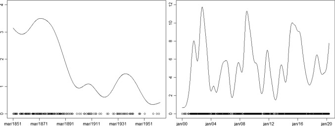
To motivate the use of GMMPPs we consider two real data sets regarding coal mining disasters and the exchange rate between Brazilian Real (BRL) and US Dollar (USD). For the former, each event represents an explosion that killed ten or more men in Britain. For the latter, each event represents a day in which the variation w.r.t. the previous day was greater than 1%. A kernel method (see Diggle 1985) is used to estimate the IF as it is shown in Fig. 1 and suggests that the IF ought to be well described, in both examples, by a GMMPP with an increasing and a decreasing line with varying starting values. Both examples are revisited in Sect. 5.
Fig. 1.
Two real data sets and the respective empirical IF. Left: Coal mining disasters—time unit is year. Right: daily variation over 1% in the BRLxUSD exchange rate—-time unit is month
Finally, we propose a specific model to fit epidemic curves, allowing for asymmetry between the growth and decay behaviors. The model allows for simplifications in the proposed MCMC algorithm, which lead to reasonable computational times even for very large data sets—with more than 300 thousand observations. The model is applied to data sets regarding Dengue Fever epidemics in Brazil and the COVID-19 pandemic. This is presented in “Appendix E”.
Other examples of point process models that do not assume the stochastic independence property of Poisson processes, are the self-exciting Hawkes process (Rasmussen 2013, see, for example) and the Matérn repulsive process (Rao et al. 2017, see, for example).
This paper is organized as follows. Sections 2 and 3 present the GMMPP and the MCMC algorithm, respectively. Section 4 explores simulated examples to discuss the efficiency of the methodology and compare it to a non-parametric Cox process approach, in terms of inference and computational cost. Finally, Sect. 5 applies the methodology to real datasets. Two of them are the ones presented in Fig. 1 regarding coal mining disasters and the BRLxUSD exchange rate.
Generalized Markov modulated Poisson processes
Let be a non-homogeneous Poisson process (NHPP) with intensity function and consider K functional forms , . These may be, for example, constants, increasing or decreasing lines, exponential functions, etc. The IF switches among the different functional forms according to the transitions of a continuous-time Markov chain , with Q-matrix , initial distribution and state space , for , where is the vector of parameters indexing . Furthermore, in its most general form, we allow the IF to switch from the same functional form to itself and have different starting values every time a functional form is revisited. We call the resulting process Y a generalized Markov modulated Poisson process with mathematical representation given as follows.
Define , as the jump times of X and as the corresponding sequence of visited states, i.e. , , and . For each s, the surjective function assigns a functional form to each of the states of X and . Additionally, , with , is the value of the IF at and is a vector of parameters indexing the ’s. The generalized Markov modulated Poisson process is formally defined as follows.
| 1 |
| 2 |
| 3 |
| 4 |
We can set any subset of the functional forms (from none to all of them) to allow for self-jumps—the ith jump is a self-jump if . This way, the size of the state space E can be anything from K to 2K. Some choices for the prior on R are presented in Sect. 3. For example, suppose that is a straight line with slope , then, for a given s such that the IF assumes the functional form at , we have that .
The IF can be interpreted in two ways: i) a discrete time Markov chain and a sequence of exponentially distributed random variables as well as initial values R, from which a piecewise deterministic function is constructed; ii) a piecewise deterministic Markov process conditioned on the values of a discrete time Markov chain. Naturally, the IF is required to be non-negative. Formally, we deal with this issue by assigning zero to the density of Y conditional on any trajectory of the IF that assumes negative values.
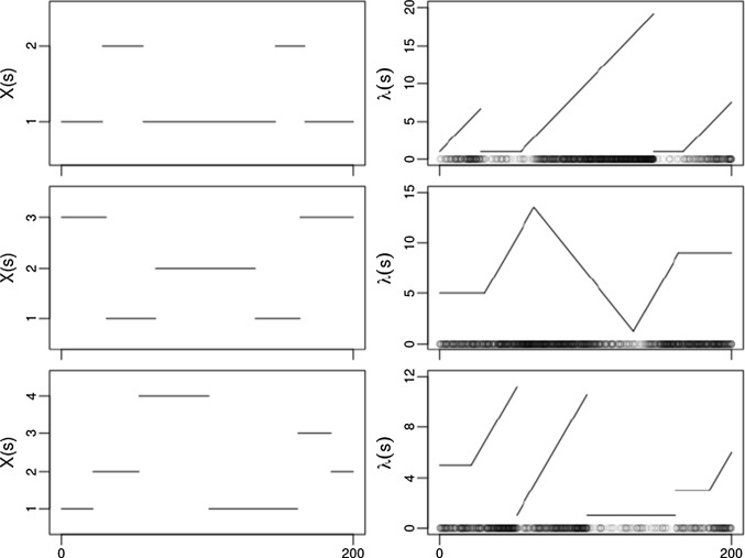
In the simpler case in which the IF is not allowed to switch from each to itself, we set , . On the other hand, if that feature is allowed, we set , . In order to favor model identifiability in a statistical context, some entries of the matrix are set to be zero so that a jump to the kth functional form that is not a self-jump can only happen through the kth state of X and never through the th one. Figure 2 illustrates the proposed class of models by presenting a realization for three examples of GMMPPs.
Fig. 2.
Three examples of GMMPPs. Left: CTMC trajectory, right: IF trajectory and generated PP events (circles). Each example considers, respectively, one of the three possible priors on R presented in Sect. 3. Self-jumps are allowed on the third example
Bayesian inference
We aim at performing inference for GMMPPs based on the observation of the process over a finite time interval [0, S]. The inference process consists in obtaining the posterior distribution of the intensity function and unknown parameters. Given the structure of the proposed class of models, this is equivalent to the distribution of , where y represents a realization of the process Y in [0, S]. In order to fully specify the model under the Bayesian approach we need to assign a prior distribution to parameters and . We define , where is the set of parameters indexing the kth functional form, as the rates of the waiting times of X and as the transition probabilities from the states corresponding to the kth functional form. The parameter vectors and are assumed to be independent a priori. Independence among all the ’s and among the components of and vectors is also assumed. In the case that no self-jumps are allowed, the full prior specification of is completed by setting, for ,
| 5 |
If self-jumps are allowed, each row of has K non-zero probabilities due to the restrictions imposed to have model identifiability. Moreover, the transition probabilities between the two states corresponding to the same functional form are the same and the transition probabilities between the th and th functional forms are the same when moving from either of the two states corresponding to the th form to state . This means that there are K transition probabilities associated to each functional form and the vector of these probabilities are assumed to follow a Dirichlet distribution, i.e.,
| 6 |
for .
The rate parameters of the waiting times are set to be the same for the two states corresponding to the same functional form for which self-jumps are allowed. In order to illustrate all the restrictions imposed to the matrix, consider an example with three functional forms, all allowed to self-jump. The resulting matrix is then given by
We consider a few options for the prior of the set R of starting values. Note that the (random) dimension of R is , where |T| is the size of T in [0, S]. One possible choice for the prior on R is to fix the starting value of each functional form to be the same on every visit to that form. This implies that the initial value of each functional form is a parameter indexing that form and, if this is unknown, it is added to the parameter vector . We call this the prior 1 for R.
Another option for the prior on (prior 2) is a point-mass distribution depending on that leads to a continuous IF trajectory, being therefore closer in form to the traditional log Gaussian Cox process. This prior is defined by
| 7 |
A third option (prior 3) assumes
| 8 |
for some distribution , . This means that all the starting values referring to the same functional form are independent and identically distributed. Furthermore, in order to have a feasible MCMC algorithm, the constant functional form is the only one for which a continuous prior can be adopted, in particular, a gamma distribution. For all the other forms, a discrete prior must be adopted and, unless useful information is available, we shall assume uniform discrete priors on supports chosen according to the scale of the IF. A more flexible approach is to fix the size of the support of this discrete distribution but set the actual values to be unknown and assuming a joint continuous prior.
Model elicitation and identifiability
The proposed class of GMMPPs offers a considerably flexible structure to model a variety of point process phenomena. This flexibility, however, gives rise to complex important issues that have a great influence on the quality of the statistical analysis. More specifically, model and prior elicitation should be carefully performed to avoid identifiability problems and favor a reasonable model fit. Reliable prior information about the phenomenon under study should always be used to elicit informative priors. One may also consider a preliminary analysis of the data and the use of informative priors. A non-parametric kernel estimate of the density function can be used to guide the choice of the functional forms and other features of the model, like self-jumps and prior structure of the initial values.
The use of informative priors should be considered based on the (prior) information acquired. For example, if few transitions are expected, the data would provide little information about the parameters indexing the matrix. In this case, the information that few transitions are expected could be used to elicit informative priors for the mean waiting time parameters in terms of the scale of the model (magnitude of the waiting times). Moreover, scenarios in which the IF is estimated to have few transitions will be weakly informative about parameters indexing the Q-matrix, yielding a low predictive power. On the other hand, if the IF is estimated to have a considerable number of transitions, reasonable information about the Q-matrix will be available and, in turn, reasonably precise predictions can be made. Finally, prior information may also be used to elicit informative priors for the parameters .
Generally speaking, the proposed class of models does not aim at emulating non-parametric structures, which would imply the need for many functional forms with short visits to each one. This would compromise model identifiability and computational cost. The actual aim is to provide good model fitting and prediction with high gains in terms of computational cost in situations in which a non-parametric structure for the IF is expendable.
All of the issues discussed above are explored in the simulated and real examples presented in Sects. 4 and 5.
Model augmentation and the MCMC algorithm
The target posterior distribution of is highly complex, which suggests the use of MCMC methods as the most reasonable choice to perform inference. Developing an efficient algorithm, however, is not straightforward and should consider non-trivial techniques to achieve that goal. We consider a model augmentation approach similar to the one used in Rao and Teh (2013) but with some adaptations to gain computational efficiency. The model augmentation is based on the augmented representation of a CTMC introduced in Hobolth and Stone (2009) and referred to as uniformization. The CTMC is represented as a discrete time Markov chain (DTMC) subordinated to a Poisson process. This means that the times of the DTMC, which has the same state space of the CTMC X, are defined by a Poisson process. The augmented component comes from the fact that the DTMC may have transitions between the same state. We shall refer to those transitions as virtual jumps.
The difference between our approach and the one in Rao and Teh (2013) is that we consider a non-homogeneous Poisson process instead of a homogeneous one. The gain in efficiency due to the use of a non-homogeneous PP will be made clear further ahead in the text. The representation using non-homogeneous PP is also used in Rao and Teh (2012) in the context of inference for semi-Markov jump processes. Nevertheless, the authors do not provide a proof for the result.
Let us start by defining K constants such that , where is the kth diagonal element of . Now let be a sequence of discrete random variables on and a sequence of random times on . For , we define the following stochastic process:
| 9 |
| 10 |
| 11 |
| 12 |
for , where is a discrete distribution on E with probability vector , is the jth row of and is a row vector of size E with the jth element being 1 and all the others being 0.
As it is stated in Proposition 1 below, the process , where , subordinated to times W is an alternative representation for the CTMC X. We shall refer to this process as the augmented CTMC. Note that the virtual times are an extra component that is not defined in the original definition of a CTMC. Finally, note that the result is valid for but, in order to use this representation in our MCMC context, the strict inequality is required. This is because the equality implies the almost surely non-existence of virtual jumps, which, in turn, precludes the validity of the MCMC algorithm. This argument will be made clear further ahead in the text.
Proposition 1
For any , the process defines the same continuous time Markov chain X with initial distribution and Q-matrix .
Proof
See “Appendix A”.
Consider now the augmented model that replaces the CTMC X in the original model in (1)–(4) by the augmented CTMC defined in (9)–(12)—its graphical representation is presented in Fig. 3 and Table 5 in “Appendix B” presents an overview of the model. We define U and T as the virtual and non-virtual jump times of the augmented CTMC, respectively. The vector of all the unknown quantities in the augmented model is , where is V at times T. This means that the aim of the inference procedure is to obtain the posterior distribution of . Note that there are redundancies in the definition of since and , nevertheless, that is required due to the particular sampling scheme to be adopted in the MCMC.
Fig. 3.
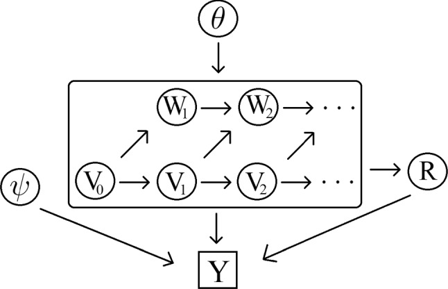
Graphical representation of the proposed augmented GMMPP model
Table 7.
Overview of the proposed augmented GMMPP
| Component | Description | Prior |
|---|---|---|
| Y | Observed Poisson process | |
| kth functional form | ||
| V | States of the DTMC that determines the functional forms of the IF of Y | |
| W | Times of the DTMC that determines the functional forms of the IF of Y | |
| T | Non-virtual jump times of the DTMC—indicate an actual change in the IF | |
| U | Virtual jump times of the DTMC | |
| R | A set with the initial value of the IF at each of the non-virtual jump times | 1. Continuous prior when the initial value is the same in all visits of each functional form. 2. Degenerate conditional prior to guarantee a continuous trajectory for the IF. 3. Continuous prior for the constant functional form and discrete prior for each of all the others when the initial value varies among visits to the same |
| Inverse of the mean waiting time of the IF at | Gamma | |
| ’ | Vector of transition probabilities from to each of the K functional forms | Dirichlet |
| Parameters indexing the functional forms | Various |
We design a Gibbs sampling algorithm, with a Metropolis-Hastings (MH) step for one of the blocks. Each block is iteratively sampled conditioned on all the other components appearing in . The blocking scheme and sampling algorithms to be adopted aim at simultaneously optimizing the convergence properties and computational cost of the algorithm. We consider the following blocks: (U, W, V); ; ; .
We present the joint density of which is useful to derive the algorithms to sample from each block. We have that
| 13 |
where each density above is obtained w.r.t. some suitable dominating measure. The likelihood is written w.r.t. the probability measure of a Poisson process with constant positive rate such that
| 14 |
where is the number of events from y in [0, S] and is the time of the nth event. The densities , and can be obtained from (9)–(12), (7)–(8) and (5)–(6), respectively. Finally, is some suitable continuous density.
Sampling (U, W, V)
First note that, conditional on , (U, W, V) is independent of the data and consists of the virtual jumps. These are sampled directly from their full conditional distribution, which is given by the following proposition.
Proposition 2
Defining as the virtual jumps in , with and , the full conditional distribution of the virtual jumps is such that:
-
i.
the ’s are mutually independent;
-
ii.
for , is a homogeneous Poisson process with rate , where is the state of V at .
Proof
See “Appendix A”.
Note that, if , the number of virtual jumps is almost surely zero and, as a consequence, the MCMC chain is reducible since the non-virtual jumps would be restricted to the set defined by its initial value. In fact, the values of the ’s have a great impact on the efficiency of the algorithm. If these are increased, the mean number of virtual jumps also does, which, in turn, improves the mixing of the chain. On the other hand, an increase in the number of virtual jumps leads to an increase in the computational cost of each iteration of the algorithm, in particular, on the step where is sampled. Rao and Teh (2013) suggests the use of in the context of inference for MMPP, based on empirical results. Note however that the authors consider a unique for all k, as presented in the original augmented CTMC representation of Hobolth and Stone (2009). This leads to different local mixing properties of the MCMC with respect to different states (in our case, different functional forms) of the CTMC. Moreover, an optimal local choice w.r.t. the state (functional form) with the larger ought to penalize the local computational cost associated to the other states. That issue is the main motivation for us to propose the alternative augmented CTMC with distinct ’s. It allows for a finer optimization of the chain’s properties in the sense of globally optimizing the mixing without penalizing the computational cost. Finally, based on the results of Rao and Teh (2013), we set for all k.
The original algorithm from Rao and Teh (2013) may also benefit from the use of distinct dominating rates , for the same reasons discussed in the previous paragraph. The step to sample the virtual jumps would be performed according to the result in Proposition 2 and, therefore, be identical to the same step in our algorithm. The other step, in which the states of the subordinated Markov chain are sampled, would be performed by the FFBS algorithm proposed in the original paper but considering the jth row of the transition matrix of the subordinated Markov chain to be .
Sampling
The full conditional density of is proportional to (13), hence
where , (l) is the number of non-virtual jumps up to and are all the starting values up to (which are not necessarily l values). Also,
Direct sampling from the full conditional distribution of requires the computation of its probability mass function, which is a (at least) -dimensional vector. Therefore, in the majority of cases, the computational cost associated to this algorithm is impractical. Furthermore, note that, for GMMPP’s, each likelihood term depends on V and R up to time , because of the dependence on the last non-virtual jump up to . For that reason, unlike in the case of inference for MMPP’s (see Rao and Teh 2013), an FFBS scheme cannot be devised to sample from the full conditional distribution of . Instead, we propose an independent Metropolis Hastings step with a proposal distribution that aims at approximating the target full conditional by adding suitable normalizing constant terms for each of the |W| terms or , accordingly. More specifically,
| 15 |
where is the normalizing constant of and is the normalizing constant of . Note that when corresponds to a virtual jump, is the constant that normalizes .
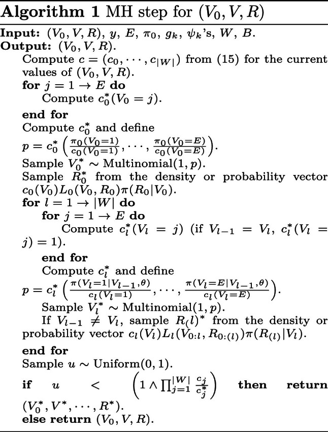
The acceptance probability of the MH step is given by
| 16 |
where the ’s and ’s refer to the current and proposal values, respectively. Note that any trajectory that leads to negative values for the IF is rejected with probability 1.
As described before, the constant functional form is the only one for which we assume a continuous prior for its starting values—a gamma prior. For all the other forms, the required normalizing constants above would typically be intractable for continuous priors. The detailed algorithm to perform the MH step described above is presented in Algorithm 1 of “Appendix B”. The algorithm for the simpler case with no varying starting value is obtained by applying straightforward simplifications.
We use the general result from Mengersen and Tweedie (1996) to establish the uniform ergodicity of the proposed MH sub-chain.
Proposition 3
The Metropolis-Hastings sub-chain defined by (15) and (16) is uniformly ergodic.
Proof
See “Appendix A”.
Since this is an independent MH algorithm, its efficiency relies heavily on its acceptance rate—the higher the better. Note that this rate should be reduced as the number of non-virtual jumps increases. For that reason, we propose an adaptation of the algorithm by partitioning the interval [0, S] and separately sampling in each of these time intervals. In order to have a robustly efficient algorithm, we propose an adapting strategy that starts by updating in one block and then partitions this into more blocks if required. The adaptation is considered up to a certain iteration of the Markov chain so to guarantee its convergence. Finally, the algorithm to sample in each sub-interval of time is a direct and straightforward adaptation of Algorithm 1 that is presented in “Appendix B”.
The partitioning strategy ought to be executed with care in order to guarantee that the respective full conditional distribution depends on the likelihood only inside the respective time interval. This means that the limits of the intervals have to be times ’s of non-virtual jumps and the proposal distribution is truncated so that the upper limit of the respective time interval remains as a non-virtual jump time and does not change the initial functional form of the next time interval. For a partition , the blocks are defined by the intervals , , , , .
The adapting partition strategy goes as follows. Set a number of iterations M large enough to obtain a reliable estimate of the acceptance rate and a reasonable threshold r for the rate. The algorithm starts with one block . Then, after every M iterations, the acceptance rate in those last M iterations is evaluated. If this rate is smaller than r, we make . The adaptation carries on until the computed rate is larger than r. Following the results from Lee and Neal (2018), we suggest . A partition with B blocks is defined by setting the intervals’ limits to be the ’s which are the closest to the times .
Finally, the continuous time Markov chain trajectory may be highly correlated with some parameters in , which may compromise the mixing of those parameters. A simple and efficient way to mitigate this problem is to perform multiple updates of (U, W, V) and on each iteration of the Gibbs sampling. This issue is illustrated in the simulated examples.
Sampling and
It is straightforward to simulate from the full conditional distribution of given the conditional independence structure and conjugation of its prior. The full conditional distribution of is a , where and are the total number of visits to and the total time spent at the kth functional form in [0, S], respectively. Moreover has a Dirichlet full conditional distribution with parameter vector , if self-jumps are allowed, and , if no self-jumps are allowed, where is the total number of transitions from functional form to functional form in [0, S],
Concerning parameters , we have from (13) that its full conditional density is
The prior independence among the ’s implies the conditional independence of the respective K full conditionals. Moreover, for a constant with fixed starting value, a leads to a full conditional
where is the number of events from y occurring during the time that the IF assumes the functional form . For all the other functional forms we perform MH steps with an adapted random walk proposal (see Roberts and Rosenthal 2009, Section 2) for each vector . The acceptance probability for each is given by
where and are the current and proposal values, respectively, and is proportional to the product of the likelihood in (14) and the prior density of .
Prediction
Prediction is a common procedure associated with the statistical analysis of stochastic processes. In the context of unidimensional Poisson processes, prediction consists in estimating the future behavior of the process, in particular, its intensity function and/or events. The Bayesian approach allows for the prediction to be made under a probabilistic approach through the predictive distribution. Consider the full Bayesian model of a GMMPP Y in and let y be a realization of the process in [0, S]. Now define to be some measurable function, in the probability space of the full Bayesian model, that depends on (Y, V, T) only in . Then, prediction about is made through the predictive distribution of .
In an MCMC context, it is straightforward to obtain a Monte Carlo (MC) sample from the predictive distribution as long as it is feasible to simulate from the full model. An MC sample is obtained by simulating conditional on each value simulated along the MCMC (after a burn-in period) due to the fact that
Appealing examples of include:
-
i.
, for ;
-
ii.
;
-
iii.
.
For examples i. and ii., it is enough to simulate the CTMC X conditional on each sample of and compute g for the respective sampled value of . For example iii., an extra step is required to simulate from a distribution, conditional on each simulated valued of .
Simulated examples
This section presents a collection of simulated examples to explore important issues related to the methodology proposed in this paper. In particular, we explore: 1. the impact of the number of observations and the number of jumps in the IF on the computational cost of the MCMC algorithm; 2. a sensitivity analysis for the priors of and ; 3. the efficiency in estimation and prediction (with replications).
Convergence diagnostics are obtained based on the MCMC chain for the parameters, for some functions of the CTMC and for the log-posterior density (logarithm of the non-normalized posterior density). Computational cost is evaluated in terms of the average time (in seconds) to obtain 100 effective samples of the log-posterior density. We consider the running time including the calibration of the MH proposal for and the adapting partition of [0, S] to sample . The effective sample size of an MCMC sample of size n is defined as , where is the autocorrelation of order j of the chain. It is such that the variance of the ergodic average of the n values from the chain is the same as the variance of the ergodic average of an independent sample (from the target distribution) of size . The sum in the denominator is truncated at the last lag for which the autocorrelation is significantly different from zero (based on an asymptotic confidence interval). For the four examples in which the GMMPP is compared to a non-parametric IF model, we consider the effective samples of the log-likelihood instead of the log-posterior density.
All the examples are implemented in Ox (Doornik 2007) and run on an i7 3.4GHz processor with 16MB RAM. Codes are available at https://github.com/liviadutra/bayesian-inference-for-gmmpp.
Investigating the computational cost
In this section, we investigate the computational cost associated to the proposed methodology. In particular, we investigate the impact of the number of observations and the number of changes in the IF trajectory. As emphasized before, the low computational cost is at the core of the main contributions of this paper.
The cost as a function of the number of observations
We simulate five scenarios with the same behavior for the IF (functional forms and changes) in the same time interval but with different levels of magnitude. We consider three functional forms—increasing and decreasing lines and a constant, with fixed starting values and no self-jumps allowed. Table 1 presents the specific functional forms, length of stay, mean number and actual number of observations. We fix the Q-matrix so that all the states have a mean staying time of 20 units and uniformly distributed transition probabilities. Multiple updates of blocks (U, W, V) and are performed to control the high autocorrelation of the parameters of the increasing line functional form—5 updates for scenarios A1 and A2, 15 for A3 and A4 and 25 for A5. Moderately informative priors are adopted for in scenario A1, namely (intercept of the increasing line), (slope of the increasing line), (intercept of the decreasing line), (slope of the decreasing line), (constant). For all the other scenarios, independent uniform improper priors are used for all parameters but , for which a Gamma(1, 1) is also used.
Table 1.
The cost as a function of the number of observations
| Scen. | ||||||||||
|---|---|---|---|---|---|---|---|---|---|---|
| Stay | Stay | Stay | ||||||||
| A1 | 0.5 | 0.25 | [36.5, 50] | 6 | - 0.25 | [0, 14.2) | 0.5 | [14.2, 36.5) | 100.68 | 103 |
| A2 | 2.5 | 1.25 | [36.5, 50] | 30 | - 1.25 | [0, 14.2) | 2.5 | [14.2, 36.5) | 503.38 | 512 |
| A3 | 10 | 5 | [36.5, 50] | 120 | - 5 | [0, 14.2) | 10 | [14.2, 36.5) | 2013.5 | 1985 |
| A4 | 50 | 25 | [36.5, 50] | 600 | - 25 | [0, 14.2) | 50 | [14.2, 36.5) | 10,068 | 9991 |
| A5 | 150 | 75 | [36.5, 50] | 1800 | - 75 | [0, 14.2) | 150 | [14.2, 36.5) | 30,203 | 30,113 |
Description of the five scenarios simulated—, length of stay, mean and actual number of observations
Results regarding the estimation of the IF and are presented in Fig. 13 and Tables 6 and 7 in “Appendix C”. They already show a reasonably good recovery of the IF and parameters for the dataset with only 103 observations, with the estimation improving substantially with the size of the dataset. MCMC diagnostics are presented in Figs. 16 and 17 in “Appendix D”.
Fig. 13.
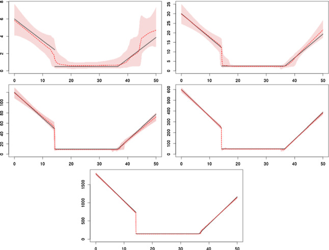
True and estimated (posterior mean and pointwise 95% CI) intensity function for scenarios A in Sect. 4.1, ordered by row
Table 5.
Posterior statistics of the parameters for scenarios A and B in Sect. 4.1
| Scen. | Parameter | True value | Mean | SD | 95% CI |
|---|---|---|---|---|---|
| A1 | 0.5 | 1.38 | 1.02 | (0.08, 3.91) | |
| 0.25 | 0.38 | 0.28 | (0.02, 1.15) | ||
| 6 | 5.84 | 0.92 | (4.18, 7.81) | ||
| − 0.25 | − 0.27 | 0.11 | (− 0.50, − 0.06) | ||
| 0.5 | 0.60 | 0.25 | (0.22, 1.04) | ||
| A2 | 2.50 | 3.07 | 2.31 | (0.16, 8.79) | |
| 1.25 | 1.45 | 0.29 | (0.94, 2.10) | ||
| 30.00 | 29.86 | 2.63 | (24.83, 35.13) | ||
| − 1.25 | − 1.20 | 0.30 | (− 1.78, − 0.64) | ||
| 2.50 | 2.35 | 0.35 | (1.71, 3.07) | ||
| A3 | 10 | 13.75 | 6.67 | (2.47, 27.43) | |
| 5 | 4.50 | 0.52 | (3.41, 5.45) | ||
| 120 | 119.15 | 5.37 | (108.83, 129.65) | ||
| − 5 | − 4.68 | 0.60 | (− 5.85, − 3.50) | ||
| 10 | 9.03 | 0.64 | (7.82, 10.31) | ||
| A4 | 50 | 40.81 | 13.65 | (19.79, 67.81) | |
| 25 | 24.69 | 0.94 | (22.83, 26.46) | ||
| 600 | 597.80 | 11.89 | (574.64, 621.42) | ||
| − 25 | − 24.88 | 1.30 | (− 27.45, − 22.31) | ||
| 50 | 47.66 | 1.47 | (44.83, 50.59) | ||
| A5 | 150 | 202.53 | 24.65 | (129.16, 240.98) | |
| 75 | 72.54 | 1.84 | (68.95, 76.17) | ||
| 1800 | 1800.26 | 20.91 | (1759.32, 1840.96) | ||
| − 75 | − 76.16 | 2.29 | (− 80.55, − 71.65) | ||
| 150 | 144.11 | 2.48 | (139.27, 149.01) | ||
| B1 | 1.7 | 2.07 | 0.97 | (0.78, 4.81) | |
| 0.85 | 0.86 | 0.07 | (0.72, 0.98) | ||
| 20.4 | 19.47 | 1.15 | (17.20, 21.68) | ||
| − 0.85 | − 0.79 | 0.10 | (− 0.97, − 0.57) | ||
| 1.7 | 1.50 | 0.21 | (1.11, 1.95) | ||
| 0.066 | 0.07 | 0.03 | (0.02, 0.14) | ||
| 0.066 | 0.09 | 0.04 | (0.03, 0.17) | ||
| 0.066 | 0.07 | 0.05 | (0.01, 0.20) | ||
| (1/3, 1/3, 1/3) | (0.24, 0.50, 0.26) | (0.16, 0.18, 0.17) | – | ||
| (1/3, 1/3, 1/3) | (0.39, 0.32, 0.29) | (0.22, 0.17, 0.20) | – | ||
| (0.5, 0.5) | (0.71, 0.29) | (0.22, 0.22) | – | ||
| B2 | 1 | 1.15 | 0.52 | (0.44, 2.57) | |
| 0.5 | 0.49 | 0.03 | (0.43, 0.55) | ||
| 12 | 11.68 | 0.67 | (10.36, 12.96) | ||
| − 0.5 | − 0.47 | 0.06 | (− 0.59, − 0.35) | ||
| 1 | 1.07 | 0.12 | (0.84, 1.29) | ||
| 0.066 | 0.07 | 0.02 | (0.03, 0.13) | ||
| 0.066 | 0.08 | 0.03 | (0.03, 0.15) | ||
| 0.066 | 0.09 | 0.04 | (0.04, 0.19) | ||
| (1/3, 1/3, 1/3) | (0.23, 0.22, 0.55) | (0.15, 0.13, 0.17) | – | ||
| (1/3, 1/3, 1/3) | (0.37,0.25,0.38) | (0.21, 0.16, 0.21) | – | ||
| (0.5, 0.5) | (0.72, 0.28) | (0.16, 0.16) | – | ||
| B3 | 0.5 | 0.68 | 0.22 | (0.29, 1.15) | |
| 0.25 | 0.25 | 0.02 | (0.20, 0.29) | ||
| 6 | 5.88 | 0.26 | (5.39, 6.39) | ||
| − 0.25 | - 0.24 | 0.02 | (− 0.28, − 0.20) | ||
| 0.5 | 0.43 | 0.06 | (0.32, 0.54) | ||
| 0.066 | 0.09 | 0.02 | (0.05, 0.15) | ||
| 0.066 | 0.09 | 0.02 | (0.05, 0.13) | ||
| 0.066 | 0.07 | 0.03 | (0.03, 0.14) | ||
| (1/3, 1/3, 1/3) | (0.12, 0.47, 0.41) | (0.09, 0.14, 0.14) | – | ||
| (1/3, 1/3, 1/3) | (0.55, 0.25, 0.20) | (0.17, 0.14, 0.14) | – | ||
| (0.5, 0.5) | (0.67, 0.33) | (0.18, 0.18) | – |
Table 6.
Posterior statistics for the number of CTMC jumps (jumps) and time of the first change in the IF () for scenarios A and B in Sect. 4.1
| True value | Mean | SD | ||
|---|---|---|---|---|
| A1 | jumps | 2 | 2.68 | 0.93 |
| 14.2 | 14.28 | 3.74 | ||
| A2 | jumps | 2 | 2.29 | 0.59 |
| 14.2 | 14.43 | 1.1 | ||
| A3 | jumps | 2 | 2.13 | 0.45 |
| 14.2 | 14.13 | 0.74 | ||
| A4 | jumps | 2 | 2.16 | 0.45 |
| 14.2 | 14.18 | 0.43 | ||
| A5 | jumps | 2 | 2.02 | 0.20 |
| 14.2 | 14.18 | 0.42 | ||
| B1 | jumps | 10 | 14.23 | 2.48 |
| 12.8 | 8.23 | 5.47 | ||
| B2 | jumps | 20 | 30.34 | 5.96 |
| 23.6 | 16.53 | 8.94 | ||
| B3 | jumps | 40 | 67.0 | 9.14 |
| 12.4 | 10.03 | 5.56 |
Fig. 16.
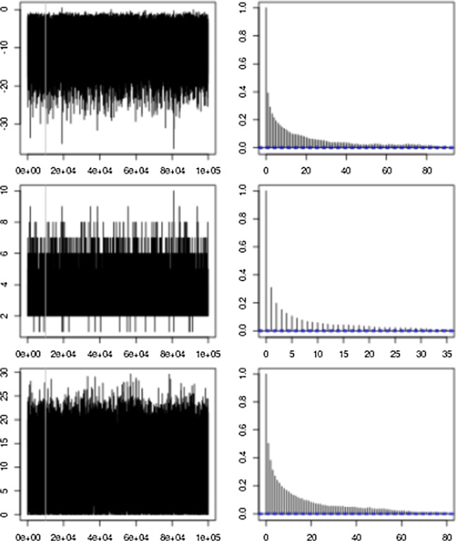
Trace plot and autocorrelation plot for the log-posterior density, number of CTMC jumps and time of the first change in the IF, respectively, for scenario A1 in Sect. 4.1
Fig. 17.
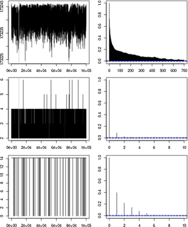
Trace plot and autocorrelation plot for the log-posterior density, number of CTMC jumps and time of the first change in the IF, respectively, for scenario A5 in Sect. 4.1
The relation between the computational cost and the number of observations is shown in Fig. 4. We highlight the computational efficiency of the proposed MCMC algorithm shown by the running times. The methodology has shown to be quite efficient to be applied for very large datasets. For example, the total running time to obtain an effective sample size of 100 for the log-posterior density is around 2.3 min for the dataset with 10 thousand observations and 18 min for the dataset with 30 thousand observations.
Fig. 4.
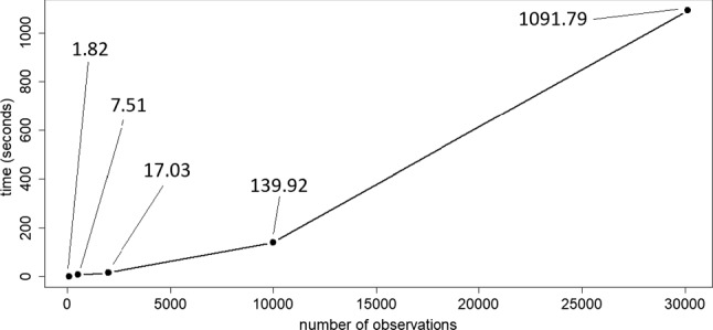
Computational cost, measured in terms of the time per 100 effective samples of the log-posterior density, versus the number of observations
The cost as a function of the number of changes in the IF
We simulate three scenarios with the same average number of observations and three functional forms—increasing and decreasing lines and a constant, with fixed starting values and self-jumps allowed. The IF is simulated from the same CTMC prior but considering different total observed time in order to have considerably different numbers of changes in the IF. The number of observations is approximately 2 thousand for all the scenarios. Table 2 presents the specific functional forms, average length of stay per visit and number of changes in the IF. The priors on the Q-matrix diagonal parameters are , and and, for the transition probability vectors, we adopt a uniform prior on the respective simplex. Finally, uniform improper priors are adopted for all the parameters. Blocks (U, W, V) and are updated 5 times in each iteration of the Gibbs sampling.
Table 2.
The cost as a function of the number of changes in the IF
| Scen. | |T| | |||||||||
|---|---|---|---|---|---|---|---|---|---|---|
| Av. st. | Av. st. | Av. st. | ||||||||
| B1 | 1.7 | 0.85 | 15 | 20.4 | - 0.85 | 15 | 1.7 | 15 | 10 | 2013 |
| B2 | 1 | 0.5 | 15 | 12 | - 0.5 | 15 | 1 | 15 | 20 | 2004 |
| B3 | 0.5 | 0.25 | 15 | 6 | - 0.25 | 15 | 0.5 | 15 | 40 | 1991 |
Description of the three scenarios simulated—, average length of stay per visit, number of changes in the IF and number of observations
Results regarding the estimation of the IF and of the and parameters are presented in Fig. 14 and Tables 6 and 7 in “Appendix C”. They show a very good recovery of the IF and parameters. MCMC diagnostics are presented in Figs. 18 and 19 in “Appendix D”.
Fig. 14.
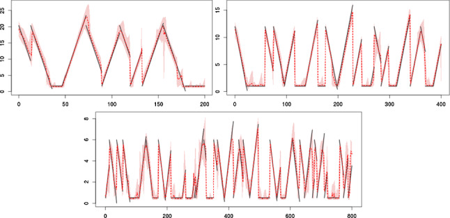
True and estimated (posterior mean and pointwise 95% CI) intensity function for scenarios B in Sect. 4.1, ordered by row
Fig. 18.
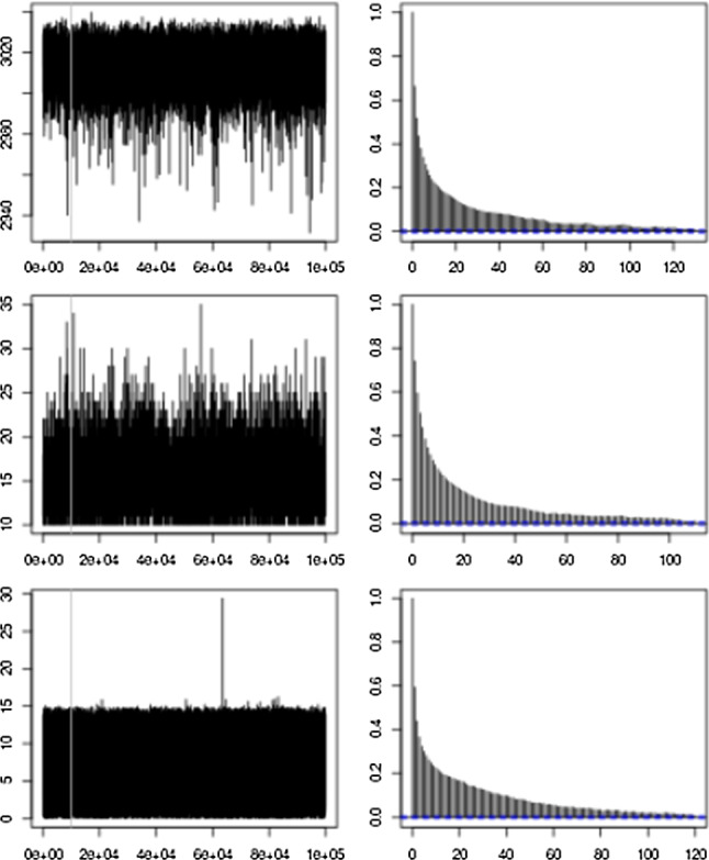
Trace plot and autocorrelation plot for the log-posterior density, number of CTMC jumps and time of the first change in the IF, respectively, for scenario B1 in Sect. 4.1
Fig. 19.
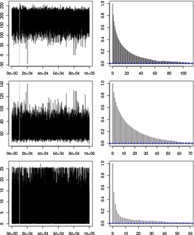
Trace plot and autocorrelation plot for the log-posterior density, number of CTMC jumps and time of the first change in the IF, respectively, for scenario B3 in Sect. 4.1
The relation between the computational cost and the real number of changes in the IF is shown in Fig. 5. Again, we highlight the computational efficiency of the proposed MCMC algorithm shown by the running times. The total running time to obtain an effective sample size of 100 for the log-posterior density is around 105 s for the dataset with 40 changes in the IF and approximately 2 thousand observations.
Fig. 5.
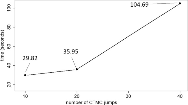
Computational cost, measured in terms of the time per 100 effective samples of the log-posterior density, versus the number of changes in the IF
Prior sensitivity analysis
We perform a prior sensitivity analysis for parameters for scenarios A1, A3, A5 and B2. Those examples are run with non-informative and moderately informative priors. The latter ones are set based on the scale of each example. Also, a prior sensitive analysis for parameters in the diagonal of the Q-matrix is performed for scenarios B1 and B3. Again, non-informative and moderately informative priors are used.
In the first analysis, the Q-matrix is fixed for all the scenarios at the same values as in Sect. 4.1. For scenario B2, the same non-informative priors from Sect. 4.1 are adopted. The prior on the constant IF parameter is set to be Gamma(1, 1) in all the cases. For the parameters indexing the other two functional forms, we compare the results for improper uniform priors and the moderately informative priors shown in Table 3. Results for the parameter estimation are presented in Table 8 in “Appendix C” and show that greater differences are observed only for the parameters of the increasing line. As it should be expected, the variances of those parameters are greater for the non-informative priors, for which the posterior density is also more asymmetric. Results for the IF go in the same direction, with significant differences observed only for scenario A1 in the time period associated with the increasing line. It can be noticed that the posterior distribution of the IF is more influenced by the data for the non-informative prior, as expected—see Fig. 15 in “Appendix C”.
Table 3.
Informative priors for the sensitivity analysis of
| Scen. | ||||
|---|---|---|---|---|
| A1 | ||||
| A3 | ||||
| A5 | ||||
| B2 | N(1, 1) |
Table 8.
Posterior statistics of the parameters for the examples in Sect. 4.2. Inf. and N-inf refer to informative and non-informative priors, respectively
| Scen. | Param. | True | Mean | SD | 95% CI | |||
|---|---|---|---|---|---|---|---|---|
| Inf. | N-inf. | Inf. | N-inf. | Inf. | N-inf. | |||
| A1 | 0.5 | 1.38 | 2.35 | 1.02 | 2.81 | (0.08, 3.91) | (0.11, 10.52) | |
| 0.25 | 0.38 | 0.47 | 0.28 | 0.52 | (0.02, 1.15) | (0.03, 2.20) | ||
| 6 | 5.84 | 5.73 | 0.92 | 0.96 | (4.18, 7.81) | (4.05, 7.77) | ||
| − 0.25 | - 0.27 | - 0.26 | 0.11 | 0.12 | (− 0.50, − 0.06) | (− 0.47, − 0.05) | ||
| 0.5 | 0.60 | 0.69 | 0.25 | 0.18 | (0.22, 1.04) | (0.36, 1.07) | ||
| A3 | 10 | 11.03 | 13.75 | 4.25 | 6.67 | (3.29, 19.02) | (2.47, 27.43) | |
| 5 | 4.68 | 4.50 | 0.42 | 0.52 | (3.88, 5.50) | (3.41, 5.45) | ||
| 120 | 119.4 | 119.15 | 5.18 | 5.37 | (109.3, 129.7) | (108.83, 139.65) | ||
| − 5 | - 4.72 | - 4.68 | 0.59 | 0.60 | (− 5.86, − 3.56) | (− 5.85, − 3.50) | ||
| 10 | 8.99 | 9.03 | 0.63 | 0.64 | (7.79, 10.28) | (7.82, 10.31) | ||
| A5 | 150 | 190.7 | 202.53 | 28.20 | 24.65 | (120.8, 230.7) | (129.16, 240.98) | |
| 75 | 73.1 | 72.54 | 1.78 | 1.84 | (69.5, 76.5) | (68.95, 76.17) | ||
| 1800 | 1800.6 | 1800.26 | 20.23 | 20.91 | (1760.5, 1840.3) | (1759.32, 1840.96) | ||
| − 75 | - 76.2 | - 76.16 | 2.22 | 2.29 | (− 80.5, − 71.8) | (- 80.55, − 71.65) | ||
| 150 | 144.1 | 144.11 | 2.47 | 2.48 | (139.3, 149.0) | (139.27, 149.01) | ||
| B2 | 1 | 1.23 | 1.15 | 0.51 | 0.52 | (0.51, 2.54) | (0.44, 2.57) | |
| 0.5 | 0.49 | 0.49 | 0.03 | 0.03 | (0.43, 0.55) | (0.43, 0.55) | ||
| 12 | 11.67 | 11.68 | 0.66 | 0.67 | (10.37, 12.97) | (10.36, 12.96) | ||
| − 0.5 | - 0.47 | - 0.47 | 0.06 | 0.06 | (− 0.60, − 0.35) | (− 0.59, − 0.35) | ||
| 1 | 1.07 | 1.07 | 0.12 | 0.12 | (0.84, 1.29) | (0.84, 1.29) | ||
| 0.066 | 0.07 | 0.07 | 0.02 | 0.02 | (0.03, 0.12) | (0.03, 0.12) | ||
| 0.066 | 0.08 | 0.08 | 0.03 | 0.03 | (0.03, 0.15) | (0.03, 0.15) | ||
| 0.066 | 0.09 | 0.09 | 0.04 | 0.04 | (0.04, 0.19) | (0.04, 0.19) | ||
Fig. 15.
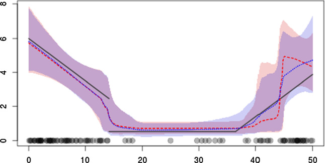
True and estimated (posterior mean and pointwise 95% CI) intensity function for scenarios A1 in Sect. 4.2 for the informative (blue) and non-informative (red) priors on . (Color figure online)
The second sensitivity analysis concerns the prior distribution on the parameters in the diagonal of the Q-matrix. Improper uniform priors are adopted for all the parameters except for the constant value which has a Gamma(1, 1) non-informative prior. Uniform priors on the simplex are adopted for all the transition probability vectors in the Q-matrix. The non-informative priors for the Q-matrix diagonal parameters are improper uniforms distributions and the informative ones are , and . Results (omitted here) are virtually the same for the two prior specifications w.r.t. the estimated IF, parameters and transition probability vectors from the Q-matrix. As for the parameters in the diagonal of the Q-matrix, small yet non-negligible differences are observed, with slightly larger variances for the case with non-informative priors.
Efficiency in estimation and prediction
Examples with replications
We now investigate the efficiency of the proposed methodology in terms of estimation and prediction by considering replications of the same model. We consider the IF from scenarios A1, A3 and B2 and generate 50 independent datasets for each one. Prediction for the integrated IF in the interval [400, 800] is performed for scenario B2 by sampling from its predictive distribution.
In order to summarize the performance of the methodology we consider the posterior distribution of the following measure of fit:
| 17 |
where is the real intensity function.
Results are shown in Figs. 6, 7 and 8 and reveal a very good performance to estimate and predict the IF.
Fig. 6.
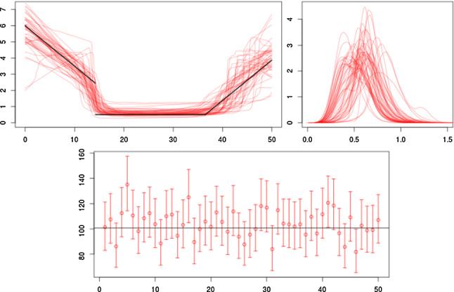
Results for 50 replications of scenario A1. Top left: true (black line) and posterior mean of the IF for each replication. Top right: posterior density of the measure of fit in (17) for each replication. Bottom: mean and 95% CI for the integrated IF for each replication. Horizontal line represents the real value
Fig. 7.
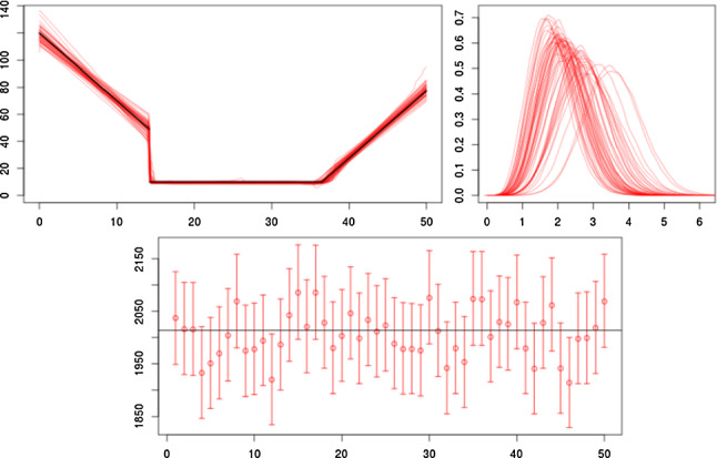
Results for 50 replications of scenario A3. Top left: true (black line) and posterior mean of the IF for each replication. Top right: posterior density of the measure of fit in (17) for each replication. Bottom: mean and 95% CI for the integrated IF for each replication. Horizontal line represents the real value
Fig. 8.
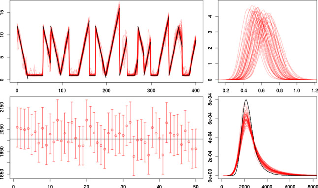
Results for 50 replications of scenario B2. Top left: true (black line) and posterior mean of the IF for each replication. Top right: posterior density of the measure of fit in (17) for each replication. Bottom left: mean and 95% CI for the integrated IF for each replication. Horizontal line represents the real value. Bottom right: real (black line) and posterior predictive density of the integrated IF in [400, 800]
Comparison to non-parametric Cox process model
We compare our methodology to that from Gonçalves and Gamerman (2018), in which the IF is assumed to be a continuous positive function of a latent Gaussian process. As it is demonstrated in that paper, this is the most computationally efficient exact methodology for Gaussian process-driven IF Cox processes. The computational cost associated to the MCMC algorithm from Gonçalves and Gamerman (2018) is , where is the supremum of the IF in [0, S]. It is defined by the cost to generate multivariate normal distributions which are required due to the use of a latent Gaussian process. This implies that not only the cost is larger and grows much faster than the cost from our methodology but also that it is not feasible to apply the methodology to very large datasets.
We consider three scenarios—C1, C2 and C3, with deterministic IFs. Scenario C1 considers a dataset of size 302 generated from the IF in [0, 50] and excluding the 8 observations generated in [9, 14] (so, there is no “true” IF). The GMMPP is fitted with decreasing and increasing lines and a constant, all with non-varying intercept (prior 1 for R). Uniform improper priors are adopted for all the parameters indexing the increasing and decreasing lines and a Gamma(1, 1) for the constant one. A prior Gamma(1, 20) is adopted for all the three diagonal parameters of the Q-matrix. The prior on the probability vectors of the Q-matrix are uniform Dirichlet. The estimated IF for both models are shown in Fig. 9.
Fig. 9.
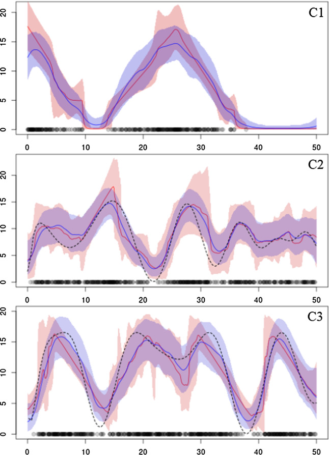
Comparison between the estimated IF (posterior mean and 95% pointwise CI) for the GMMPP (red) and the non-parametric IF (blue) models for scenarios C1, C2 and C3. Black dashed line is the true IF and circles are the observations. (Color figure online)
Scenarios C2 and C3 consider the IFs shown in Fig. 9, along with the estimated IF for both models. C2 has 452 observations and C3 has 519. The GMMPPs fitted in the C2 considers increasing and decreasing lines with varying starting values (prior 3 for R) and a non-varying constant line (prior 1 for R). C3 considers increasing and decreasing lines with varying starting value only for the former. We set priors N(1.3, 1) and for the slope of the increasing and decreasing functions in C2 and uniform discrete priors on and for the intercepts of the increasing and decreasing lines, respectively. A Gamma(1, 10) prior is adopted for all the three diagonal parameters of the Q-matrix. All of those priors basically set the scale of the IF to favor model identifiability. For C3, we set N(15, 4) for the intercept of the decreasing line, uniform improper priors for the slope parameters and a uniform discrete prior on for the intercept of the increasing line. Priors Gamma(1, 5) and Gamma(1, 10) are adopted for the two diagonal parameters of the Q-matrix, respectively. The priors on the probability vectors of the Q-matrix are uniform Dirichlet for both scenarios.
Results for the three scenarios show that similar results are obtained for the GMMPP and the non-parametric models. We also compare those models in terms of computational efficiency—see Table 4, to reinforce the computational advantages of the proposed methodology.
Table 4.
Time (in min) per 100 effective samples of the log-likelihood function
| Scenario | GMMPP | Non-parametric |
|---|---|---|
| C1 | 0.255 | 120 |
| C2 | 7.33 | 138 |
| C3 | 2.59 | 110 |
Applications
Here, we present two applications to illustrate our methodology. Furthermore, in “Appendix E”, we propose a specific model to fit epidemic curves and analyze data from Dengue Fever in Brazil and COVID-19 in Switzerland and Romania. This is a data-driven statistical approach that allows for uncertainty quantification in estimation and prediction and is computationally feasible to be applied to large datasets.
Coal mining disasters
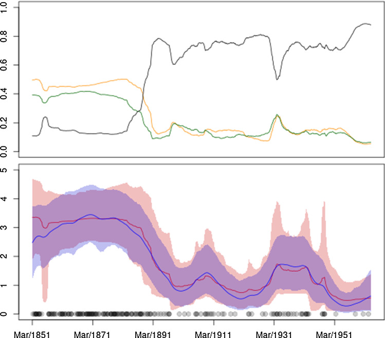
We apply the proposed methodology to the classic coal mining disasters data of Jarrett (1979), consisting of the dates of 191 explosions in coal mines that killed ten or more men in Britain between 15th March 1851 and 22nd March 1962 (re-scaled to [0, 111], year unit). We also analyze these data with the non-parametric IF model of Gonçalves and Gamerman (2018).
Based on an empirical analysis of the data (see Fig. 1), we set three functional forms—decreasing and increasing lines and a constant, all with varying starting values (prior 3 for R). We adopt the following priors: for the varying starting values of the increasing and decreasing lines and a Gamma(1, 1) for the constant; and for the slopes; the three diagonal parameters of the Q-matrix are fixed at 1/60 and the transition distributions are fixed to be uniform. The former considers the time scale of the data to penalize scenarios with expendable changes in the intensity function but without compromising its estimation.
The computational time per 100 effective samples of the log-likelihood is 3.8 min for the GMMPP and 8.6 min for the non-parametric IF model (with no approximations to simulate from the Gaussian process). The estimated IF for both models is shown in Fig. 10, along with the posterior probability of each functional form. The posterior mean of the integrated IF is 201.7 (standard deviation = 15.5) for the GMPP and 193.4 (14.5) for the non-parametric IF model. The posterior mean of the slopes are -0.0811 (0.0966) for the negative one and 0.0904 (0.1009) for the positive one.
Fig. 10.
Top: posterior probability of each functional form—constant (black), increasing line (green) and decreasing line (orange). Bottom: estimated IF for the coal mining data for the GMMPP and non-parametric IF models. Red line and pale-red shadow are the posterior mean and 95% CI for the GMPP and blue line and pale-blue shadow are the same statistics for the non-parametric model. Circles are the observations. (Color figure online)
BRLxUSD exchange rate
We consider the exchange rate between US Dollar to Brazilian Real. The dataset consists of the 1163 days, between Jan 2000 and Dec 2017 (re-scaled to [0, 216], month unit), in which the daily variation was higher than 1%. Prediction is performed for the period of Jan 2018 to Apr 2020.
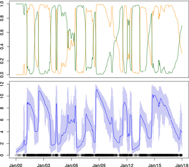
Based on an empirical analysis of the data (see Fig. 1), we set two functional forms—decreasing and increasing lines, both with varying starting values. We adopt the following priors: and for the varying starting values of the decreasing and increasing lines, respectively, and uniform improper priors for both the slopes. A Gamma(1, 40) is assumed for the diagonal parameters of the Q-matrix and uniform Dirichlet priors are used for the transition probabilities. The observed time interval is divided into 6 blocks to update the CTMC component.
The MCMC algorithm takes around 4.6 min to draw 100 effective samples. The estimated IF and the posterior probability of each functional form are shown in Fig. 11. The posterior mean and standard deviation of the integrated IF is 1143.1 and 34.3. The posterior mean of the slopes are –0.3102 (standard deviation = 0.0651) for the negative one and 0.1176 (0.0355) for the positive one. The same statistics for the mean waiting times are 11.70 (4.18) for the decreasing line and 9.36 (3.16) for the increasing line.
Fig. 11.
Top: posterior probability of each functional form—increasing line (green) and decreasing line (orange). Bottom: Estimated IF (posterior mean and 95% CI) for the exchange rate data. Circles are the observations
The predictive distribution of the integrated intensity between Jan 2018 and Apr 2020 is shown in Fig. 12 and has mean 151.4, standard deviation 35.80 and 95% CI (78.44, 218.29). The real observed number of events is 151.
Fig. 12.
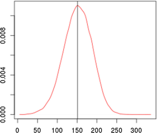
Posterior predictive density of the integrated IF for the exchange rate example. The vertical line represents the real observed number of events in the predicted period
Conclusions
This paper proposed a novel class of unidimensional Cox processes in which the intensity function assumes predefined functional forms and alternates among these according to the jumps of a continuous time Markov chain. This novel class aims at providing an efficient way to perform useful statistical analysis of unidimensional point processes at a very reasonable computational cost, especially when compared to non-parametric approaches based on latent Gaussian processes.
Important issues regarding model elicitation and identifiability and some aspects of the MCMC algorithm are discussed and explored in simulated studies. Model elicitation should be based on prior knowledge and/or empirical analysis of the data. Whilst non-informative priors work well for the parameters indexing the functional forms, prior elicitation for the parameters in the Q-matrix requires special attention. If not many changes are expected, parameters in the diagonal should be fixed at values coherent with the scale in a way to avoid very short visits. For the transition probabilities, uniform priors are suitable in any case.
The proposed MCMC algorithm performs exact Bayesian inference for GMMPPs so that only Monte Carlo error is involved. The algorithm is carefully devised to efficiently sample from the posterior distribution of all the unknown quantities in the model. In particular, the blocking scheme to sample from the CTMC trajectory has been shown to be crucial to obtain a computationally efficient algorithm. Simulated studies illustrated the computational and statistical efficiency of the proposed methodology under different circumstances. In particular, efficient solutions for large datasets are obtained at a reasonable cost.
Two real datasets are also analyzed and prediction is performed for one of them, providing good results. Finally, results indicate that, typically, models with only straight lines (increasing, decreasing and constant) are enough to provide a good fit.
Acknowledgements
The first author would like to thank FAPEMIG and CNPq for financial support. The second author would like to thank CAPES for financial support. The third author was partially supported by FAPEMIG (Universal APQ-00774-21). The authors would like to thank Fábio Demarqui for helping in obtaining the COVID19 data and Leonardo Bastos for helping in obtaining the Dengue Fever data.
Appendix A: Proofs
Proof of Proposition 1
Let be the first non-virtual jump and the state of V at . The density of with respect to the Lebesgue measure is
Similar calculations show that , , . Furthermore,
Analogous calculations establish the required result for .
Proof of Proposition 2
Clearly,
where . This gives . The result above establishes part i. of the proposition.
We now obtain the full conditional density of , , w.r.t. the measure of a unit rate Poisson process. We have that
where is the number of virtual jumps in . This establishes part ii. of the proposition for . For , we have that
which concludes the proof.
Proof of Proposition 3
In order to establish uniform ergodicity for an independent MH chain, it is enough to show that the ratio , where is the target density, is uniformly bounded away from zero on the support of (Mengersen and Tweedie 1996). Note that
where is a constant and is the support of the full conditional distribution of . The fact that , for all l, completes the proof.
Appendix B: Model and MCMC details
See Table 5.
Appendix C: Results from the simulations
Appendix D: MCMC diagnostics
Appendix E: Modeling epidemic curves
We consider a model which we believe to be of practical use to model epidemic phenomena. The idea is to model each cycle of the IF to have an exponential growth, some period of stabilization and then an exponential decay. Moreover, in order to mimic the expected behavior of epidemic curves, we need the exponential growth and decay rates to change over time. This behavior can be emulated by using a cdf as part of the functional form, in particular the standard normal cdf. The parameterization is such that the model is flexible and parameters have a clear interpretation. In order to fit the proposed model, we need either to observe an entire cycle or up to a time when the IF has already started to decrease, in which case, prediction for the remainder of the cycle may be performed. The IF is assumed to start in the increasing functional form and then having one change to the decreasing one (Figs. 18, 19). The model is the following:
where and are the increasing and decreasing curves, respectively, and is set to be to guarantee the continuity of the IF at the change time.
We impose some restrictions on the parameter space so to ease model identifiability and parameter interpretation. We set , , , and as standard identifiability restrictions. We also set the less obvious restriction so that the time period of constant behavior of the IF is more likely to be accommodated by the end of the increasing function and, consequently, identifiability of the change point is favored. Also, note that in order to estimate the stabilization level the data needs to include the stabilization period, otherwise, this parameter should be fixed (for example, at zero).
The restrictions above lead to a clear interpretation of the model’s parameters as follows.
: identifies the initial value of the IF—typically around ;
a: defines the maximum value assumed by the IF—typically ;
: defines the initial growth rate of the IF curve;
: defines the rate in which the growth curve changes and the maximum growth rate;
: defines the initial decay rate of the IF curve;
: defines the rate in which the decay curve changes and the maximum decay rate;
: defines the stabilization level after the epidemic period.
Furthermore, the maximum slope of the growth and decay curves are given by and , respectively. In order to improve the mixing of the MCMC algorithm by reducing the correlation among parameters, we reparameterize the model in terms of instead of . This implies that
| 18 |
| 19 |
| 20 |
We highlight the fact that the Bayesian approach and the variance of the Poisson process conditioned on its IF provide considerable flexibility and suitable uncertainty quantification to model epidemic curves, especially when compared to deterministic models directly applied to the number of events.
Moreover, this model can be extended to have more flexible curves by considering the cdf of other distributions such as student-t, skew-normal and skew-t. This can account, for example, for skewed growth and decay curves and for cases in which the epidemic curve decays faster than it grows up to a certain time but then takes longer to stabilize, suggesting the use of a heavy tail cdf to model the decay.
Finally, we can also consider a sequence of cycles to model epidemics with several waves. Furthermore, if a reasonable number of waves are observed, we can adopt generalized linear model priors for the waiting time parameters with covariates that help to explain it, such as social isolation indexes, hospital occupation rates, vaccination percentages, etc. This approach could then be used to forecast the future behavior of the epidemics in terms of future waves.
Inference for the epidemic model
The model in (18)–(20) has features that allow for some improvements in the MCMC from Sect. 3.2. It is now possible to sample directly from the full conditional distribution of the block at a reasonable computational cost. That is because the condition of having only one change in the IF is imposed and, therefore, the size of the state space of this discrete full conditional distribution is |W|. This also allows us to increase the value of and, consequently, improve the mixing of the chain, without compromising the cost. One may consider, for example, .
Another strategy to boost computational efficiency is to truncate the change time to be inside a suitable interval, based on the empirical IF. This interval is conservatively chosen so that it is certain that the change occurs inside it.
Dengue Fever epidemic
We analyze data from the 2019 Dengue Fever epidemic in Ceará (CE) state, Brazil, and the 2019/2020 Dengue Fever epidemic in Paraná (PR) state, Brazil. The raw data consists of the number of cases per epidemic week, from week 52 of 2018 (23/12/2018) to week 52 of 2019 (28/12/2019)—371 days, for Ceará, and from week 36 of 2019 (01/09/2018) to week 22 of 2020 (30/05/2020)—273 days, for Paraná. In order to analyze the data, we distribute the cases uniformly in their respective week and use day as the scale unit. The total number of cases in that period was 30700 in Ceará and 331411 in Paraná. The epidemic curve in Paraná is relatively close to stabilization, but still decaying, so we also predict the time until stabilization—when the IF hits 110. Data is available in the InfoDengue system (Codeco et al. 2018).
For the Ceará data, we were compelled to restrict parameter a to be in the interval (0, 250)—safely higher than the maximum of the empirical IF, in order to avoid the growth curve to be fit by only (around) half of the cdf. This avoids identifiability and computational problems. For parameter we set priors Uniform for Ceará and Uniform(0, 3) for Paraná. Uniform improper priors are adopted for all the other parameters. The diagonal values of the Q-matrix are fixed at (1/120, 1/250), for Ceará, and (1/180, 1/90), for Paraná. Results are shown in Fig. 20 and Table 9.
Fig. 20.
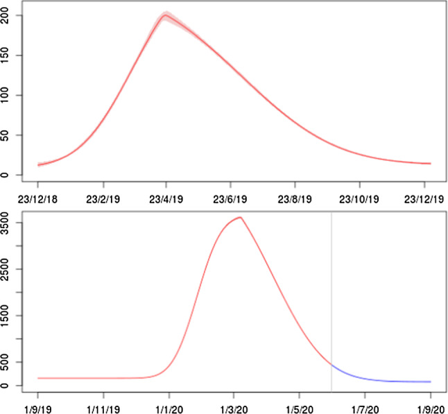
Estimated IF (posterior mean and 95% CI (red) and predictive mean and 95% predictive interval (blue)) for the Dengue Fever data—Ceará (top) and Paraná (bottom). (Color figure online)
Table 9.
Posterior statistics for the Dengue Fever and COVID-19 models
| a | IIF | Pred. Time | Pred. IIF | ||||||||
|---|---|---|---|---|---|---|---|---|---|---|---|
| CE | Mean | 248.3 | 8.80 | 2.47 | - 2.22 | 12.78 | 1.25 | 0.99 | 30558.3 | – | – |
| s.d. | 1.67 | 2.04 | 0.082 | 0.088 | 1.00 | 0.024 | 0.13 | 174.2 | – | – | |
| PR | Mean | 3510.4 | 154.2 | 77.5 | - 8.17 | 80 | 46.6 | 0.785 | 331541 | 314.4 (July 12th) | 9266.8 |
| s.d. | 18.9 | 1.28 | 0.66 | 0.087 | - | 0.282 | 0.043 | 574.7 | 0.80 | 242.0 | |
| Swi. | Mean | 1295.7 | 10.20 | 98.11 | -4.16 | 22.14 | 36.14 | 0.64 | 30548.9 | – | – |
| s.d. | 4.06 | 1.51 | 1.81 | 0.07 | 1.55 | 0.84 | 0.096 | 169.5 | – | – | |
| Rom. | Mean | 358.6 | 0.78 | 19.14 | - 4.00 | 0 | 5.77 | 0.66 | 19137.6 | 147.9 (July 23rd) | 3096.3 |
| s.d. | 10.10 | 0.36 | 0.47 | 0.11 | - | 0.31 | 0.46 | 138.4 | 7.44 | 471.6 |
IIF is the integrated IF in the observed interval, Pred. time is the predictive time at which the IF reaches 110 and Pred. IIF is the predictive integrated IF until that time
COVID-19 epidemic
We also analyze data from the Covid-19 pandemic in Switzerland and Romania. Whilst the epidemic curve has already stabilized for the former, it is still decaying for the latter. For that reason, we predict the time until stabilization—when the IF hits 20, for Romania. The dataset for Switzerland concerns the 30845 cases notified from Feb 25th (date of the first notification) to May 30th—96 days. The dataset from Romania concerns the 19133 cases notified from Feb 26th (date of the first notification) to May 30th—95 days. Data is obtained from the Coronavirus Resource Center of John Hopkins University through the R package covid19br (Demarqui and Santos 2020).
For the Switzerland data, we restrict parameter a to be in the interval (0, 1300) for the same reasons we restrict that parameter for the Ceará Dengue Fever data. For parameter we set priors Uniform for Switzerland and Uniform(0, 3) for Romania. Uniform improper priors are adopted for all the other parameters. The diagonal values of the Q-matrix are fixed at (1/30, 1/60), for Switzerland, and (1/50, 1/40), for Romania. Results are shown in Fig. 21 and Table 9.
Fig. 21.
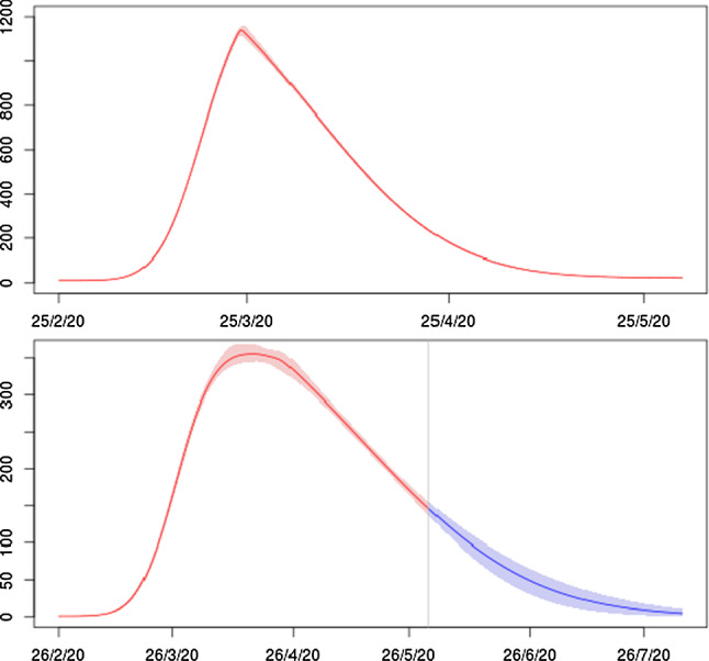
Estimated IF [posterior mean and 95% CI (red) and predictive mean and 95% predictive interval (blue)] for the COVID-19 data—Switzerland (top) and Romania (bottom). (Color figure online)
Footnotes
Publisher's Note
Springer Nature remains neutral with regard to jurisdictional claims in published maps and institutional affiliations.
References
- Adams, R.P., Murray, I., Mackay, D.J.C.: Tractable nonparametric Bayesian inference in Poisson processes with Gaussian process intensities. In: Proceedings of the 26th International Conference on Machine Learning (ICML 2009) (2009)
- Codeco, C., Coelho, F., Cruz, O., Oliveira, S., Castro, T., Bastos, L.: Infodengue: a nowcasting system for the surveillance of arboviruses in Brazil. Revue d’Épidémiologie et de Santé Publique 66, S386 (2018). European Congress of Epidemiology Crises, epidemiological transitions and the role of epidemiologists
- Demarqui, F.N., Santos, C.C.: covid19br. R package (2020)
- Diggle P. A kernel method for smoothing point process data. J. R. Stat. Soc. Ser. C. 1985;34:138–147. [Google Scholar]
- Doornik JA. Object-Oriented Matrix Programming Language Ox. 3. London: Timberlake Consultants Press and Oxford; 2007. [Google Scholar]
- Fearnhead P, Sherlock C. An exact Gibbs sampler for the Markov-modulated Poisson process. J. R. Stat. Soc. Ser. B Stat. Methodol. 2006;68(5):767–784. doi: 10.1111/j.1467-9868.2006.00566.x. [DOI] [Google Scholar]
- Gonçalves FB, Gamerman D. Exact Bayesian inference in spatiotemporal Cox processes driven by multivariate Gaussian processes. J. R. Stat. Soc. Ser. B. 2018;80:157–175. doi: 10.1111/rssb.12237. [DOI] [Google Scholar]
- Gonçalves, F.B., Łatuszynski, K., Roberts, G.O.: Exact Bayesian inference for diffusion driven Cox processes. ArXiv:2007.05812 (2020)
- Hobolth A, Stone EA. Simulation from endpoint-conditioned, continuous-time Markov chains on a finite state space, with applications to molecular evolution. Ann. Appl. Stat. 2009;3(3):1204. doi: 10.1214/09-AOAS247. [DOI] [PMC free article] [PubMed] [Google Scholar]
- Jarrett RG. A note on the intervals between coal-mining disasters. Biometrika. 1979;66:191–193. doi: 10.1093/biomet/66.1.191. [DOI] [Google Scholar]
- Lee C, Neal P. Optimal scaling of the independence sampler: theory and practice. Bernoulli. 2018;24:1636–1652. doi: 10.3150/16-BEJ908. [DOI] [Google Scholar]
- Mengersen KL, Tweedie RL. Rates of convergence of the Hastings and Metropolis algorithms. Ann. Stat. 1996;24(1):101–121. doi: 10.1214/aos/1033066201. [DOI] [Google Scholar]
- Møller J, Syversveen AR, Waagepetersen RP. Log Gaussian Cox processes. Scand. J. Stat. 1998;25:451–482. doi: 10.1111/1467-9469.00115. [DOI] [Google Scholar]
- Rao V, Adams RP, Dunson DB. Bayesian inference for Matérn repulsive processes. J. R. Stat. Soc. Ser. B. 2017;79:877–897. doi: 10.1111/rssb.12198. [DOI] [Google Scholar]
- Rao, V., Teh, Y.W.: MCMC for continuous-time discrete-state systems. In: Advances in Neural Information Processing Systems 25 (NIPS 2012) (2012)
- Rao V, Teh YW. Fast MCMC sampling for Markov jump processes and extensions. J. Mach. Learn. Res. 2013;14(1):3295–3320. [Google Scholar]
- Rasmussen JG. Bayesian inference for Hawkes processes. Methodol. Comput. Appl. Probab. 2013;15:623–642. doi: 10.1007/s11009-011-9272-5. [DOI] [Google Scholar]
- Roberts GO, Rosenthal JS. Examples of adaptive MCMC. J. Comput. Graph. Stat. 2009;18(2):349–367. doi: 10.1198/jcgs.2009.06134. [DOI] [Google Scholar]
- Walder, C.J., Bishop, A.: Ofast Bayesian intensity estimation for the permanental process. In: Proceedings of the 34th International Conference on Machine Learning (ICML 2017) (2017)


