Relative efficiency of equal versus unequal cluster sizes in cluster randomized trials with a small number of clusters

Abstract

To calculate sample sizes in cluster randomized trials (CRTs), the cluster sizes are usually assumed to be identical across all clusters for simplicity. However, equal cluster sizes are not guaranteed in practice, especially when the number of clusters is limited. Therefore, it is important to understand the relative efficiency (RE) of equal versus unequal cluster sizes when designing CRTs with a limited number of clusters. In this paper, we are interested in the RE of two bias-corrected sandwich estimators of the treatment effect in the Generalized Estimating Equation (GEE) models for CRTs with a small number of clusters. Specifically, we derive the RE of two bias-corrected sandwich estimators for binary, continuous, or count data in CRTs under the assumption of an exchangeable working correlation structure. We consider different scenarios of cluster size distributions and investigate RE performance through simulation studies. We conclude that the number of clusters could be increased by as much as 42% to compensate for efficiency loss due to unequal cluster sizes. Finally, we propose an algorithm of increasing the number of clusters when the coefficient of variation of cluster sizes is known and unknown.

1. Introduction

When designing a cluster randomized trial (CRT) to compare an active treatment against a placebo, researchers need both the number of clusters and the cluster size (number of individuals per cluster) to achieve the desired power for testing the efficacy of the active treatment. For simplicity, the cluster sizes are often assumed to be identical across all clusters. If the cluster size is a pre-specified number, then the sample size calculation is for the number of clusters; or if the number of clusters is a pre-specified number, then the sample size calculation is for cluster sizes. However, equal cluster sizes are not guaranteed in practice. For example, the Dominantly Inherited Alzheimer Network (DIAN) enrolls the biological adult children of a parent with a very rare mutated gene (Presenilin1, Presenilin2 or Amyloid Beta Precursor Protein (APP)), which is known to cause dominantly inherited Alzheimer’s disease (DIAD). The number of individuals from each family (cluster) has a significantly skewed distribution, ranging from 1 to more than 10. Further, because of the limited number of families carrying these rare mutations, it is impossible to seek other families with similar family sizes. Therefore, CRTs with unequal family sizes will be designed on the DIAN. To handle the unequal cluster sizes in designing CRTs, the coefficient of variation (CV) of cluster sizes has been used in the equations of sample size for CRTs (Donner et al., 1981; Liu et al., 1997; Shih, 1997; Rosner et al., 2003; Eldridge et al., 2006; Austin, 2007; Candel et al., 2008; Van Breukelen et al., 2008; Teerenstra et al., 2010; Rosner et al., 2011; Van Breukelen et al., 2012; Amatya et al., 2013). Further, researchers have also investigated the relative efficiency (RE) of equal versus unequal cluster sizes when testing the treatment effect (Manatunga et al., 2001; Van Breukelen et al., 2007; Candel et al., 2010; Liu et al., 2018). They have concluded that there is a significant efficiency loss from unequal cluster sizes, and that additional clusters are needed to compensate for such a loss.

The generalized estimating equation (GEE) models proposed by Liang and Zeger (Liang et al., 1986) are often used in CRTs to incorporate the correlated nature of clustered data. When the number of clusters is large, e.g., over 40, the empirical sandwich estimator of the covariance matrix obtained from the GEE works well. However, its challenge is the bias in the covariance estimator when there are a limited number of clusters (Kauermann et al., 2001; Mancl et al., 2001; O'Brien et al., 2004). Therefore, bias-corrected sandwich estimators have been proposed to improve performance in the GEE approach (Fay et al., 2001; Kauermann et al., 2001; Mancl et al., 2001; Morel et al., 2003; Westgate et al., 2016). Whereas the performance of the bias-corrected sandwich estimators has been investigated under the assumption of identical cluster size from a small number of clusters, it remains an open question as to how these estimators perform with both unequal cluster sizes and a small number of clusters. In this paper, we study the treatment effect in CRTs with a small number of clusters in a two-group setting but with three common types of efficacy measures: binary, continuous, and count outcomes. We consider two bias-corrected sandwich estimators, an MD-corrected estimator (Mancl et al., 2001) and FG-corrected estimator (Fay et al., 2001), and derive the variances of the treatment effect for equal and unequal cluster sizes. We investigate the performance of RE for different scenarios of cluster size distributions with a small number of clusters through simulation studies. We estimate the number of clusters that must be increased to account for efficiency loss. Our previous work considered the empirical sandwich estimator in the RE derivation (Liu et al. 2018), however, we focus on bias-corrected sandwich estimators in this paper.

The outline of this article is as follows. Section 2 derives the variance of the estimator of the treatment effect in two bias-corrected estimators for binary, continuous, and count outcomes in a two-group CRT and introduces the RE of equal versus unequal cluster sizes for the treatment effect. Section 3 presents the simulation designs about cluster size distributions and the results of RE through the simulations. In Section 4, we compare the number of clusters between our proposed algorithm and the available formulas for binary outcomes. Section 5 illustrates how to apply the proposed algorithm using a real DIAN study, followed by a discussion about the directions for future research.

2. Bias-corrected sandwich estimators

Let ${\mathit{y}}_i=(y_{i1},y_{i2},\cdots ,y_{i{n}_i}{)}^{\prime }$ be a vector of responses from the ith cluster, i = 1, ⋯, m. The responses are assumed to be independent across clusters but correlated within each cluster. The marginal model is

$$g\left({\mu }_{ij}\right)={\mathbf{C}}_{ij}^{\prime }\mathbf{\varnothing },i=1,\cdots ,m;j=1,\cdots ,n_i,$$

where μ_ij = E(y_ij) and g(⋅) is a linking function. C_ij is a vector of covariates, and ∅ is an unknown l × 1 vector of regression coefficients. This model specifies a relationship between μ_ij and covariates C_ij. The conditional variance of y_ij given C_ij is defined as var (y_ij|C_ij) = γ(μ_ij, where μ is a known variance function of μ_ij and θ is a scale parameter. The mean of y_i is denoted by μ_ij = E(y_i) and the variance-covariance matrix for y_i is denoted by ${\mathit{V}}_i=\theta {\mathit{A}}_i^{1/2}{\mathit{R}}_i\left(\mathrm{\rho }\right){\mathit{A}}_i^{1/2}$, where ${\mathit{A}}_i=\mathrm{d}\mathrm{i}\mathrm{a}\mathrm{g}\left\{\gamma \left({\mu }_{i1}\right),\cdots ,\gamma \left({\mu }_{i{n}_i}\right)\right\}$ and working correlation structure R_i(ρ) describes the pattern of measures within the ith cluster. With the assumption of exchangeable working correlation structure, ${{{\mathbf{1}}_{n_i}^{\prime }\mathbf{R}}_i^{-1}1}_{n_i}=\frac{n_i}{1+(n_i-1)\mathrm{\rho }}=\frac{n_i}{{\lambda }_i},$ where ${\mathbf{1}}_{n_i\times n_i}$ is a n_i × n_i matrix of 1’s and λ_i = 1 + (n_i − 1)ρ.

Liang and Zeger (Liang et al., 1986) proved that $\sqrt{m}(\widehat{\mathit{\varnothing }}-\mathit{\varnothing })$ is asymptotically multivariate normal with mean 0 and covariance matrix ${\mathit{V}}_{\mathit{R}}=\underset{m\to \infty }{\lim }m\left({\mathbf{\Sigma }}_1^{-1}{\mathbf{\Sigma }}_0{\mathbf{\Sigma }}_1^{-1}\right),$ where $\widehat{\mathit{\varnothing }}$ is an estimator obtained by solving GEE, ${\mathit{D}}_i=\partial {\mathit{\mu }}_i/\partial {\mathit{\varnothing }}^{\prime },$ ${\mathit{V}}_i=\theta {\mathit{A}}_i^{1/2}{\mathit{R}}_i\left(\mathrm{\rho }\right){\mathit{A}}_i^{1/2}$ is a working covariance matrix of ${\mathit{y}}_i,{\mathbf{\Sigma }}_1=\sum _{i=1}^m{\mathit{D}}_i^{\prime }{\mathbf{V}}_i^{-1}{\mathit{D}}_i$ and ${\mathbf{\Sigma }}_0=\sum _{i=1}^m{\mathit{D}}_i^{\prime }{\mathbf{V}}_i^{-1}\mathrm{c}\mathrm{o}\mathrm{v}\left({\mathit{y}}_{\mathit{i}}\right|{\mathbf{C}}_i){\mathbf{V}}_i^{-1}{\mathit{D}}_i$. Typically, $\left({\mathit{y}}_{\mathit{i}}-{\widehat{\mathit{\mu }}}_{\mathit{i}}\right)({\mathit{y}}_{\mathit{i}}-{\widehat{\mathit{\mu }}}_{\mathit{i}}{)}^{\mathrm{T}}$ is used to estimate Cov(y_i|C_i) in the GEE approach (Kauermann et al., 2001; Mancl et al., 2001; O'Brien et al., 2004; Westgate et al., 2016). This empirical sandwich estimator of the covariance matrix works well when the number of clusters is large, e.g., at least 40. The small-sample performance of GEE has been investigated and simulations have shown that the empirical sandwich estimator tend to be liberal (Paik, 1988; Emrich et al., 1992; Gunsolley et al., 1995; Feng et al., 1996; Mancl et al., 2001). The simulation studies conducted by Paik for first-order autoregressive gamma responses and by Feng et al (Feng et al., 1996) for multivariate normal responses have shown that the empirical sandwich estimator tends to underestimate the variance of regression coefficients to a varying degree when the number of clusters is less than 50. Therefore, bias-corrected sandwich estimators have been proposed to improve performance in the GEE approach (Fay et al., 2001; Kauermann et al., 2001; Mancl et al., 2001; Morel et al., 2003; Westgate et al., 2016). The simulations in the work of Li and Redden suggest that no bias-corrected sandwich estimator is consistently better than the others when the Wald t-test is used in the CRTs with few clusters (Li et al., 2015). They also showed that the MD-corrected sandwich estimator should be cautiously used when the number of clusters is less than 20. In short, there is no consensus about using these bias-corrected estimators in two-level CRTs.

In this paper, we focus on the MD-corrected estimator (Mancl et al., 2001) and the FG-corrected estimator (Fay et al., 2001). The main interest is to test the treatment effect for a two-group comparison: treated versus control groups. For simplicity, let us consider a special case with l = 2, where ∅ = (β₀, β₁)′. The hypotheses of interest are H₀: β₁ = 0 versus H₁: β₁ = β. The sample size is determined by testing these hypotheses at a given treatment effect β₁ with pre-specified levels of type I error and power.

2.1. MD-corrected sandwich estimator

When the number of clusters is small, Mancl et al (Mancl et al., 2001) proposed the MD-corrected estimator which approximates the variance of $\widehat{\mathit{\varnothing }}$ by

$${\mathit{V}}_{\mathrm{M}\mathrm{D}}={\mathbf{\Sigma }}_1^{-1}{\mathbf{\Sigma }}_{\mathrm{M}\mathrm{D}}{\mathbf{\Sigma }}_1^{-1},$$ (1)

where ${\mathbf{\Sigma }}_{\mathrm{M}\mathrm{D}}=\sum _{i=1}^m{\mathit{D}}_i^{\prime }{\mathbf{V}}_i^{-1}\left({{\mathit{I}}_i-\mathit{H}}_i{)}^{-1}\mathrm{c}\mathrm{o}\mathrm{v}\left({\mathit{y}}_{\mathit{i}}|{\mathbf{X}}_i\right)\right({{\mathit{I}}_i-\mathit{H}}_i{)}^{-1}{\mathbf{V}}_i^{-1}{\mathit{D}}_i,$ I_i is an n_i × n_i identity matrix, and ${\mathit{H}}_i={\mathit{D}}_i{\mathbf{\Sigma }}_1^{-1}{\mathit{D}}_i^{\prime }{\mathbf{V}}_i^{-1}$. The n_i × n_i matrix H_i is an expression for the leverage of the ith cluster. For the purpose of sample size calculation at the design stage, we need to assume values for the variance and covariance of y_i. Under the assumption of cov (y_i|X_i) = V_i, we have ${\mathbf{\Sigma }}_{\mathrm{M}\mathrm{D}}=\sum _{i=1}^m{\mathit{D}}_i^{\prime }{\mathbf{V}}_i^{-1}\left({{\mathit{I}}_i-\mathit{H}}_i{)}^{-1}{\mathit{V}}_i\right({{\mathit{I}}_i-\mathit{H}}_i{)}^{-1}{\mathbf{V}}_i^{-1}{\mathit{D}}_i.$

We follow the proof in the work of Liu et al (Liu et al., 2018). For binary outcomes, ${\mathbf{\Sigma }}_1=\left(\begin{array}{cc}{\mathrm{\Sigma }}_t+{\mathrm{\Sigma }}_o& {\mathrm{\Sigma }}_t\\ {\mathrm{\Sigma }}_t& {\mathrm{\Sigma }}_t\end{array}\right),$ where $p_0=\frac{\exp \left({\beta }_0\right)}{1+\exp \left({\beta }_0\right)},p_1=\frac{\exp \left({\beta }_0+{\beta }_1\right)}{1+\exp \left({\beta }_0+{\beta }_1\right)},c=\sum _{i\in \mathrm{c}\mathrm{o}\mathrm{n}\mathrm{t}}\frac{n_i}{{\lambda }_i},q=\sum _{i\in \mathrm{t}\mathrm{r}\mathrm{t}}\frac{n_i}{{\lambda }_i},{\mathrm{\Sigma }}_o=p_0\left(1-p_0\right)c,{\mathrm{\Sigma }}_t=p_1\left(1-p_1\right)q,$ $i\in \mathrm{t}\mathrm{r}\mathrm{t}$ denotes all clusters assigned to treated group, and i ∈ cont denotes all clusters assigned to control group, respectively. For this MD-corrected estimator, we also derive the leverage of the ith cluster H_ii. For the clusters in the control group, through some matrix computation, ${\mathit{H}}_i=a_i{\mathbf{1}}_{n_i\times n_i}$ and then $({{\mathit{I}}_i-\mathit{H}}_i{)}^{-1}={\mathit{I}}_i+\frac{a_i}{1-a_i{n}_i}{\mathbf{1}}_{n_i\times n_i},$ where $a_i=\frac{1}{{\lambda }_{i}c}.$ Further, we have

$${\mathit{D}}_i^{\prime }{\mathbf{V}}_i^{-1}({{\mathit{I}}_i-\mathit{H}}_i{)}^{-1}{\mathit{V}}_i({{\mathit{I}}_i-\mathit{H}}_i{)}^{-1}{\mathbf{V}}_i^{-1}{\mathit{D}}_i=r_i\left[\begin{array}{cc}1& 0\\ 0& 0\end{array}\right],$$

where $r_i=p_0\left(1-p_0\right)\frac{n_i}{{\lambda }_i{\left(1-a_i{n}_i\right)}^2}.$ Similarly, for the clusters in the treated group, we have

$${\mathit{H}}_i=\frac{1}{b_i}{\mathbf{1}}_{n_i\times n_i},{\mathit{D}}_i^{\prime }{\mathbf{V}}_i^{-1}({{\mathit{I}}_i-\mathit{H}}_i{)}^{-1}{\mathit{V}}_i({{\mathit{I}}_i-\mathit{H}}_i{)}^{-1}{\mathbf{V}}_i^{-1}{\mathit{D}}_i=s_i\left[\begin{array}{cc}1& 1\\ 1& 1\end{array}\right],$$

where $b_i=\frac{\mathbf{1}}{{\lambda }_{i}q},$ and $s_i=p_1\left(1-p_1\right)\frac{n_i}{{{\lambda }_i\left(1-b_i{n}_i\right)}^2}.$ Therefore, Equation (1) becomes

$${\mathit{V}}_{\mathrm{M}\mathrm{D}}={\mathbf{\Sigma }}_1^{-1}\left({\sum }_{i\in \mathrm{c}\mathrm{o}\mathrm{n}\mathrm{t}}{r}_i\left[\begin{array}{cc}1& 0\\ 0& 0\end{array}\right]+{\sum }_{i\in \mathrm{t}\mathrm{r}\mathrm{t}}{s}_i\left[\begin{array}{cc}1& 1\\ 1& 1\end{array}\right]\right){\mathbf{\Sigma }}_1^{-1}.$$

Thus,

$$\mathrm{Var}\left({\widehat{\beta }}_1\right)=\frac{1}{p_0\left(1-p_0\right)c^2}{\sum }_{i\in \mathrm{cont}}\frac{n_i}{{{\lambda }_i\left(1-a_i{n}_i\right)}^2}+\frac{1}{p_1\left(1-p_1\right)q^2}{\sum }_{i\in \mathrm{trt}}\frac{n_i}{{\lambda }_i{\left(1-b_i{n}_i\right)}^2}.$$ (2)

Through similar steps as above, for continuous and count outcomes, we have

$$\mathrm{Var}\left({\widehat{\beta }}_1\right)={\sigma }^2\left(\frac{1}{c^2}{\sum }_{i\in \mathrm{cont}}\frac{n_i}{{{\lambda }_i\left(1-a_i{n}_i\right)}^2}+\frac{1}{q^2}{\sum }_{i\in \mathrm{trt}}\frac{n_i}{{\lambda }_i{\left(1-b_i{n}_i\right)}^2}\right),$$ (3)

and

$$\mathrm{Var}\left({\widehat{\beta }}_1\right)=\frac{1}{{e^{{\beta }_0}c}^2}{\sum }_{i\in \mathrm{cont}}\frac{n_i}{{{\lambda }_i\left(1-a_i{n}_i\right)}^2}+\frac{1}{{e^{{\beta }_0+{\beta }_1}q}^2}{\sum }_{i\in \mathrm{trt}}\frac{n_i}{{\lambda }_i{\left(1-b_i{n}_i\right)}^2},$$ (4)

respectively. If we assume equal cluster size n_i = n for all i, then λ = 1 + (n − 1) ρ and for binary outcomes,

$$\mathrm{Var}\left({\widehat{\beta }}_1\right)=\frac{m\lambda }{n}\{\frac{(1-\pi )}{p_0(1-p_0){\left(m\left(1-\pi \right)-1\right)}^2}+\frac{\pi }{p_1(1-p_1){\left(m\pi -1\right)}^2}\},$$ (5)

for continuous outcomes,

$$\mathrm{Var}\left({\widehat{\beta }}_1\right)=\frac{m\lambda {\sigma }^2}{n}\left\{\frac{(1-\pi )}{{\left(m\left(1-\pi \right)-1\right)}^2}+\frac{\pi }{{\left(m\pi -1\right)}^2}\right\},$$ (6)

and for count data,

$$\mathrm{Var}\left({\widehat{\beta }}_1\right)=\frac{m\lambda }{n{e}^{{\beta }_0}}\left\{\frac{(1-\pi )}{{\left(m\left(1-\pi \right)-1\right)}^2}+\frac{\pi }{e^{{\beta }_1}{\left(m\pi -1\right)}^2}\right\},$$ (7)

respectively.

2.2. FG-corrected sandwich estimator

The FG estimator corrects the bias of the variance of $\widehat{\mathit{\varnothing }}$ by

$${\mathit{V}}_{\mathrm{F}\mathrm{G}}={\mathbf{\Sigma }}_1^{-1}{\mathbf{\Sigma }}_{\mathrm{F}\mathrm{G}}{\mathbf{\Sigma }}_1^{-1},$$ (8)

where ${\mathbf{\Sigma }}_{\mathrm{F}\mathrm{G}}=\sum _{i=1}^m{\mathit{K}}_i{\mathit{D}}_i^{\prime }{\mathbf{V}}_i^{-1}\mathrm{c}\mathrm{o}\mathrm{v}\left({\mathit{y}}_{\mathit{i}}|{\mathbf{C}}_i\right){\mathbf{V}}_i^{-1}{\mathit{D}}_i{\mathit{K}}_i,$ K_i is a l × l diagonal matrix with the jjth element equal to ${\left[1-\mathrm{m}\mathrm{i}\mathrm{n}(d,{\mathit{Q}}_i^{jj})\right]}^{-1/2}$, ${\mathit{Q}}_i={\mathit{D}}_i^{\prime }{\mathbf{V}}_i^{-1}{\mathit{D}}_i{\mathbf{\Sigma }}_1^{-1}$, and d is a constant defined by the user which guarantees that each diagonal element of K_i is less than or equal to 2. Fay and Graubard arbitrarily chose d = 0.75 and their simulations showed that the bound of d = 0.75 is rarely reached (Fay et al., 2001). Under the assumption of V_i = cov (y_i|C_i) Equation (8) is simplified as ${\mathbf{\Sigma }}_{\mathrm{F}\mathrm{G}}=\sum _{i=1}^m{\mathit{K}}_i{\mathit{D}}_i^{\prime }{\mathbf{V}}_i^{-1}{\mathit{D}}_i{\mathit{K}}_i.$

After some matrix computation, we have the diagonal matrix ${\mathit{K}}_i=\left[\begin{array}{cc}{k}_i^{11}& 0\\ 0& 1\end{array}\right]$ if the ith cluster is in the control group; ${\mathit{K}}_i=\left[\begin{array}{cc}1& 0\\ 0& k_i^{22}\end{array}\right]$ if the ith cluster is in the treated group, where $k_i^{11}={\left[1-\mathrm{m}\mathrm{i}\mathrm{n}(d,\frac{n_i}{c{\lambda }_i})\right]}^{-1/2}$ and $k_i^{22}={\left[1-\mathrm{m}\mathrm{i}\mathrm{n}(d,\frac{n_i}{q{\lambda }_i})\right]}^{-1/2}.$ For binary outcomes, we have

$$\mathrm{Var}\left({\widehat{\beta }}_1\right)=\frac{w_{11}}{o^2}-\frac{2}{o}\left(\frac{1}{o}+\frac{1}{e}\right)w_{12}+{\left(\frac{1}{o}+\frac{1}{e}\right)}^2{w}_{22},$$ (9)

where the expressions, e.g. o, e, are detailed in Table 1. If we assume equal cluster size n_i = n for all i, then

$$\mathrm{Var}\left({\widehat{\beta }}_1\right)=\frac{w_{11}^{eq}}{o_{eq}^2}-\frac{2}{o_{eq}}\left(\frac{1}{o_{eq}}+\frac{1}{e_{eq}}\right)w_{12}^{eq}+{\left(\frac{1}{o_{eq}}+\frac{1}{e_{eq}}\right)}^2{w}_{22}^{eq}.$$ (10)

For continuous and count outcomes, we have the same Equations (9) and (10) for the variance of the estimator of the treatment effect through the similar derivations. However, all expressions are different and also detailed in Table 1.

Table 1.

Notations

	Binary	Continuous	Count
o	p0(1 − p0)c	$\frac{1}{{\sigma }^2}c$	$e^{{\beta }_0}c$
e	p1(1 − p1)q	$\frac{1}{{\sigma }^2}q$	$e^{{\beta }_0+{\beta }_1}q$
w 11	p0(1 − p0)v11 + p1(1 − p1)q	$\frac{1}{{\sigma }^2}\left(v_{11}+q\right)$	$e^{{\beta }_0}{v}_{11}+e^{{\beta }_0+{\beta }_1}q$
w 12	p1(1 − p1)v12	$\frac{1}{{\sigma }^2}{v}_{12}$	$e^{{\beta }_0+{\beta }_1}{v}_{12}$
w 22	p1(1 − p1)v22	$\frac{1}{{\sigma }^2}{v}_{22}$	$e^{{\beta }_0+{\beta }_1}{v}_{22}$
o eq	p0(1 − p0)ceq	$\frac{1}{{\sigma }^2}{v}_{22}$	$e^{{\beta }_0+{\beta }_1}{v}_{22}$
t eq	p1(1 − p1)qeq	${\frac{1}{{\sigma }^2}c}_{\mathrm{e}\mathrm{q}}$	$e^{{\beta }_0}{c}_{\mathrm{e}\mathrm{q}}$
$w_{11}^{\mathrm{e}\mathrm{q}}$	$p_0\left(1-p_0\right)v_{11}^{\mathrm{e}\mathrm{q}}+p_1\left(1-p_1\right)q_{\mathrm{e}\mathrm{q}}$	$\frac{1}{{\sigma }^2}\left(v_{11}^{\mathrm{e}\mathrm{q}}+q_{\mathrm{e}\mathrm{q}}\right)$	$e^{{\beta }_0}{v}_{11}^{\mathrm{e}\mathrm{q}}+e^{{\beta }_0+{\beta }_1}{q}_{\mathrm{e}\mathrm{q}}$
$w_{12}^{\mathrm{e}\mathrm{q}}$	$p_1\left(1-p_1\right)v_{12}^{\mathrm{e}\mathrm{q}}$	${\frac{1}{{\sigma }^2}v}_{12}^{\mathrm{e}\mathrm{q}}$	$e^{{\beta }_0+{\beta }_1}{v}_{12}^{\mathrm{e}\mathrm{q}}$
$w_{22}^{\mathrm{e}\mathrm{q}}$	$p_1\left(1-p_1\right)v_{22}^{\mathrm{e}\mathrm{q}}$	${\frac{1}{{\sigma }^2}v}_{22}^{\mathrm{e}\mathrm{q}}$	$e^{{\beta }_0+{\beta }_1}{v}_{22}^{\mathrm{e}\mathrm{q}}$

$c=\sum _{i\in \mathrm{c}\mathrm{o}\mathrm{n}\mathrm{t}}\frac{n_i}{{\lambda }_i},q=\sum _{i\in \mathrm{t}\mathrm{r}\mathrm{t}}\frac{n_i}{{\lambda }_i},k_i^{11}={\left[1-\mathrm{m}\mathrm{i}\mathrm{n}(d,\frac{n_i}{c{\lambda }_i})\right]}^{-1/2},k_i^{22}={\left[1-\mathrm{m}\mathrm{i}\mathrm{n}(d,\frac{n_i}{q{\lambda }_i})\right]}^{-1/2},$ $v_{11}=\sum _{i\in \mathrm{c}\mathrm{o}\mathrm{n}\mathrm{t}}\frac{n_i}{{\lambda }_i}{\left(k_i^{11}\right)}^2,v_{12}=\sum _{i\in \mathrm{t}\mathrm{r}\mathrm{t}}\frac{n_i}{{\lambda }_i}{k}_i^{22},v_{22}=\sum _{i\in \mathrm{t}\mathrm{r}\mathrm{t}}\frac{n_i}{{\lambda }_i}{\left(k_i^{22}\right)}^2,$ $c_{\mathrm{e}\mathrm{q}}=\frac{nm\left(1-\pi \right)}{\lambda },q_{\mathrm{e}\mathrm{q}}=\frac{nm\pi }{\lambda },k^{11}\equiv {\left[1-\min \left(d,\frac{1}{m\left(1-\pi \right)}\right)\right]}^{-\frac{1}{2}},k^{22}\equiv {\left[1-\min \left(d,\frac{1}{m\pi }\right)\right]}^{-\frac{1}{2}},$ $v_{11}^{\mathrm{e}\mathrm{q}}=\frac{nm\left(1-\pi \right)}{\lambda }{\left(k^{11}\right)}^2,v_{12}^{\mathrm{e}\mathrm{q}}=\frac{nm\pi }{\lambda }{k}^{22},v_{22}^{\mathrm{e}\mathrm{q}}=\frac{nm\pi }{\lambda }{\left(k^{22}\right)}^2.$.

2.3. Relative efficiency of equal versus unequal cluster sizes

Let Ω_equal denote a design with equal cluster size n, and let Ω_unequal denote a design with unequal cluster sizes n_i, i = 1, ⋯ m. The total sample size is $mn=\sum _{i=1}^m{n}_i.$ We follow the definition of relative efficiency (RE) when comparing unequal to equal cluster sizes (Van Breukelen et al., 2007; Liu et al., 2018; Liu et al., R & R),

$$RE\left({\widehat{\beta }}_1\right)=\frac{\mathrm{Var}\left({\widehat{\beta }}_1\right|{\mathit{\Omega }}_{\mathrm{equal}})}{\mathrm{Var}\left({\widehat{\beta }}_1\right|{\mathit{\Omega }}_{\mathrm{unqual}})}.$$ (11)

We numerically calculate $\mathrm{R}\mathrm{E}\left({\widehat{\beta }}_1\right)$ from Equations (2)–(7) for an MD-corrected estimator and Equations (9) and (10) for an FG-corrected estimator, respectively. Please note that RE is independent of σ² for continuous outcomes and $e^{{\beta }_0}$ for count data since they are eliminated based on Equation (11). The results for binary outcomes are provided in Table 2, Figures 1–4 and Appendix Figures 1–4. The results for continuous and count data are shown in Appendix Tables 3 and 4.

Table 2.

Minimum of mean RE for the different simulation designs with p₀ = 0.2 and p₁ = 0.3

Cluster sizes n	# of clusters m	Range R	Distribution	ρ, Minimum[2] of mean RE[1]
				MD-corrected estimator	FG-corrected estimator
					d=0.1	d=0.75
5	12	n	Uniform	0, 0.91	0.16, 0.95	0.05, 0.92
			Unimodal	0, 0.95	0.16, 0.98	0.05, 0.96
			Bimodal	0, 0.88	0.16, 0.94	0.05, 0.90
			Positively Skewed	0, 0.92	0.14, 0.96	0, 0.94
			Negatively Skewed	0.05, 0.92	0.21, 0.95	0.09, 0.93
		1.2n	Uniform	0, 0.86	0.18, 0.93	0.06, 0.89
			Unimodal	0, 0.93	0.18, 0.96	0.06, 0.94
			Bimodal	0, 0.83	0.18, 0.91	0.06, 0.86
			Positively Skewed	0, 0.89	0.14, 0.95	0, 0.91
			Negatively Skewed	0.08, 0.88	0.24, 0.93	0.12, 0.89
		1.6n	Uniform	0.05, 0.75	0.24, 0.86	0.10, 0.79
			Unimodal	0.05, 0.88	0.23, 0.93	0.11, 0.90
			Bimodal	0.05, 0.68	0.23, 0.82	0.10, 0.73
			Positively Skewed	0, 0.80	0.15, 0.91	0.01, 0.85
		1.8n	Uniform	0.11, 0.67	0.28, 0.80	0.16, 0.71
			Unimodal	0.13, 0.84	0.28, 0.90	0.18, 0.86
			Bimodal	0.10, 0.58	0.28, 0.75	0.15, 0.64
			Positively Skewed	0, 0.75	0.16, 0.88	0.01, 0.81
5	24	n	Uniform	0.11, 0.94	0.17, 0.95	0.13, 0.95
			Unimodal	0.11, 0.97	0.17, 0.97	0.13, 0.97
			Bimodal	0.11, 0.93	0.18, 0.94	0.13, 0.93
			Positively Skewed	0.09, 0.96	0.16, 0.96	0.11, 0.96
			Negatively Skewed	0.14, 0.94	0.19, 0.95	0.16, 0.95
		1.2n	Uniform	0.12, 0.91	0.19, 0.93	0.14, 0.92
			Unimodal	0.13, 0.96	0.18, 0.96	0.14, 0.96
			Bimodal	0.12, 0.89	0.19, 0.91	0.14, 0.90
			Positively Skewed	0.09, 0.94	0.16, 0.95	0.11, 0.94
			Negatively Skewed	0.18, 0.91	0.23, 0.92	0.19, 0.92
		1.6n	Uniform	0.17, 0.83	0.23, 0.85	0.19, 0.84
			Unimodal	0.17, 0.91	0.23, 0.92	0.19, 0.92
			Bimodal	0.16, 0.79	0.23, 0.82	0.18, 0.80
			Positively Skewed	0.10, 0.89	0.17, 0.91	0.12, 0.90
		1.8n	Uniform	0.23, 0.76	0.29, 0.79	0.25, 0.77
			Unimodal	0.24, 0.88	0.29, 0.89	0.25, 0.89
			Bimodal	0.22, 0.70	0.29, 0.75	0.24, 0.72
			Positively Skewed	0.10, 0.86	0.18, 0.88	0.12, 0.87

^[1]The mean RE among 1000 simulations is calculated for each ρ.

^[2]The minimum of mean RE including the corresponding ρ is identified across all the values of ρ.

Figure 1.

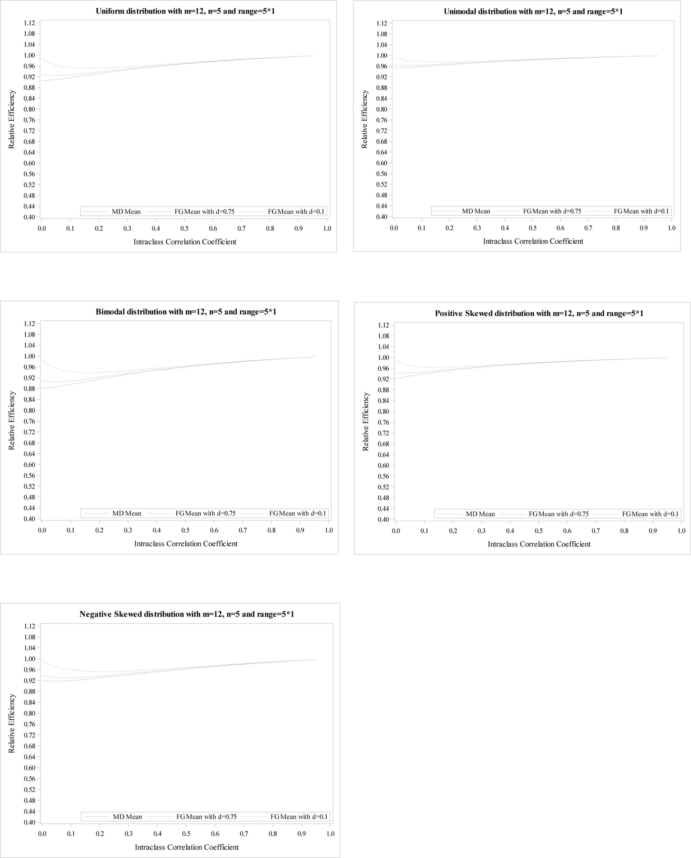
Relative efficiency of the treatment effect for five distributions with

m = 12, n = 5 and R = 5.

Figure 4.

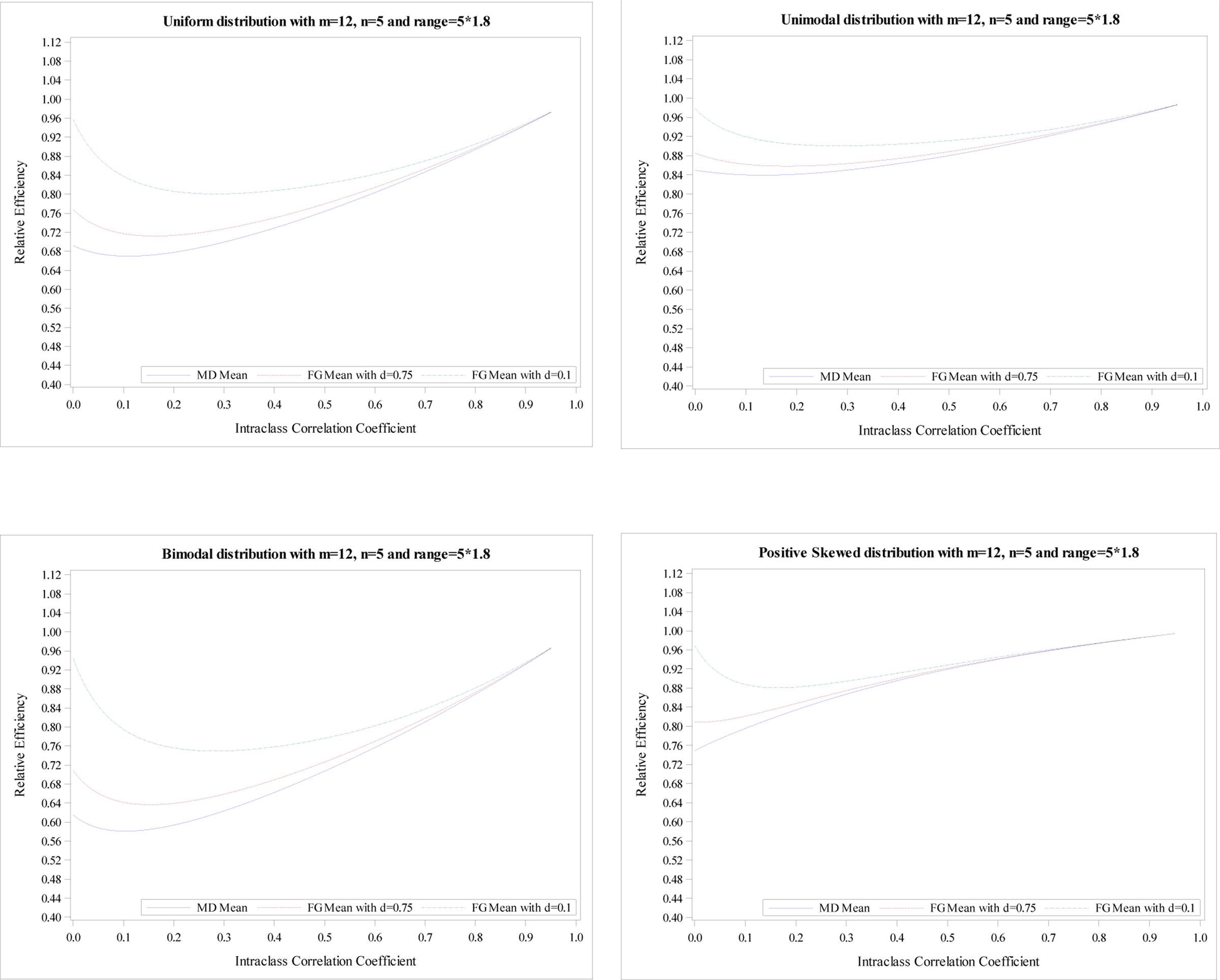
Relative efficiency of the treatment effect for five distributions with

m = 12, n = 5 and R = 5 × 1.8.

3. Simulation studies

To investigate the RE of equal versus unequal cluster sizes with a small number of clusters, we consider the following factors: (1) the number of clusters m and equal cluster size n (equivalently, total sample size N= mn); (2) the distribution of cluster size (n_i); (3) the association parameter (ρ) in the exchangeable working correlation structure; (4) the proportion of clusters allocated to the treated group π; and (5) the parameter β₁, equivalently, p_o and p₁.

We focus on a small number of clusters, so only ≤ 40 is considered. We choose the total sample size of N ≤ 3000 to reflect realistic scenarios in CRTs. Following Breukelen et al (Van Breukelen et al., 2007), we generate data using 5 distributions: a uniform, positively skewed, negatively skewed, bimodal and unimodal distribution of cluster size, respectively. Under each distribution, there are three different cluster sizes g_a < g_b < g_c, with frequencies f_a, f_b, and f_c. The parameters are detailed in Appendix Table 1. For example, for unimodal distribution, we set g_a = m/6, f_b =2m/3, f_a = m/6 and g_a = n − R/2, g_b = n, and g_c = n + R/2, given a pair value of m and n, where R can be any positive even integer. That is, m/6 clusters have cluster size of n−R/2, 2m/3 clusters have cluster size of n, and m/6 clusters have cluster size of n + R/2. Even if the intracluster correlation coefficients (ICCs) are small for most CRTs (Murray et al., 2004; Turner et al., 2004), the association parameter (ρ) ranged from 0 to 0.95 with steps of 0.01 is considered to give a comprehensive view of its impact. For all simulation study designs, we assume an equal allocation (π = 0.5) and consider p₀ = 0.2 and p₁ = 0.3, which equals β₁ = 0.539.

3.1. Designs

Given the settings shown in Appendix Table 1, the number of clusters should be a multiplier of 12 and cluster sizes should be a multiplier of 6 for an equal allocation. Thus, m = 12 and 24 are used and the cluster sizes n = 5, 30, 60, and 120 are arbitrary chosen. If a different allocation (π≠0.5) is considered, then the values of cluster sizes need to be revised correspondingly. Additionally, different ranges (R = n, 1.2n, 1.6n, 1.8n) are considered to create variation of cluster sizes. For each distribution, we have different cluster sizes if R is different. For example, if R = n and unimodal distribution, then m/6 clusters have cluster size of n/2, 2m/3 clusters have cluster size of n, and m/6 clusters have cluster size of 3n/2.

For each study design (pre-specified cluster size n, number of clusters m, range R, and cluster size distribution), the CVs of cluster size are shown in Appendix Table 2. They range from 0.29 to 0.86. Fay and Graubard (Fay et al., 2001) arbitrarily chose d = 0.75 but we set different values of d to see whether they make any RE difference. For example, when the cluster sizes are equal, we need to check $\min \left(d,\frac{1}{m\left(1-\pi \right)}\right)$ and $\min \left(d,\frac{1}{m\pi }\right).$ Under an equal allocation of $\pi =\frac{1}{2}$ and m = 12, $\frac{1}{m\left(1-\pi \right)}<0.75$ but $\frac{1}{m\left(1-\pi \right)}>0.1.$ One thousand simulation samples are generated for each design. REs are calculated using Equation (11) for both corrected estimators for all samples, and mean, standard deviation, minimum and maximum of REs are obtained at each ρ correspondingly. Source SAS code to reproduce the results is available as Supporting Information on the journal's web page (http://onlinelibrary.wiley.com/doi/xxx/suppinfo).

3.2. Results

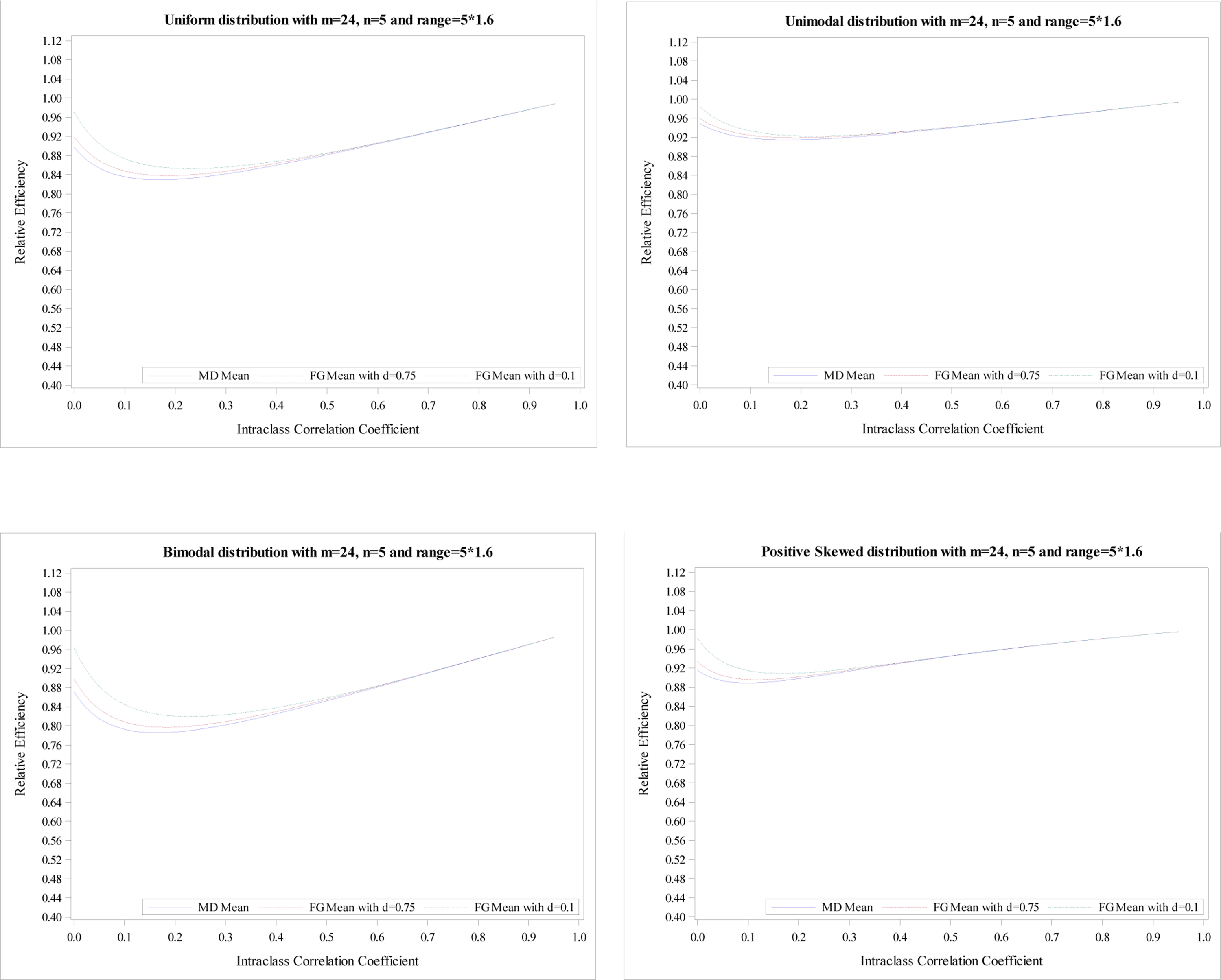
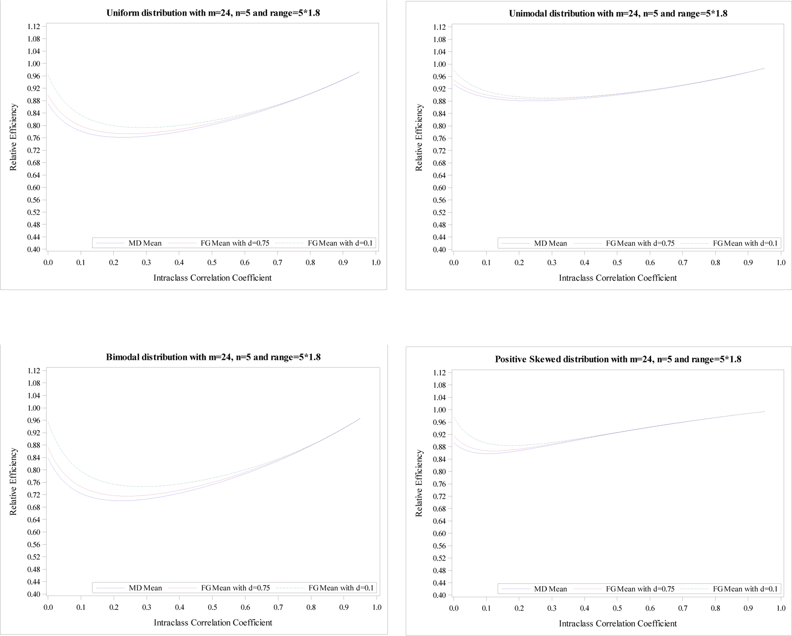
Figures 1–4 show the plots of the mean RE for two corrected estimators as a function of association parameter (ρ). Given p₀ = 0.2 and p₁ = 0.3, an MD-corrected estimator and FG-corrected estimators with d = 0.75 and d = 0.1 are presented within each figure based on simulation data with m = 12 and n = 5 for five distributions of cluster sizes, respectively. Four different ranges (R = n, 1.2n, 1.6n, 1.8n) are shown in Figures 1–4, with a small total sample size (N=60). The figures for the m = 24 are included in the Appendix. Table 2 presents the minimum of mean RE and corresponding ρ’s among 1000 repeated samples for n = 5, m = 12 and 24, four different ranges n, 1.2n, 1.6n, 1.8n), and all five distributions.

As seen in Figure 1, the mean RE from an MD-corrected estimator reaches the minimum at ρ=0, and then increases until ρ=1 for all five distributions. The minimums of mean REs are 0.91 for uniform distribution, 0.95 for unimodal distribution, 0.88 for bimodal distribution, 0.92 for positive skewed distribution, and 0.92 for negative skewed distribution, respectively. When comparing these five distributions, we find that a unimodal distribution shows the highest mean RE and a bimodal distribution shows the lowest mean RE, which is expected since unimodal distribution and bimodal distribution have the smallest and largest CV, 0.30 and 0.48. The uniform distribution has the next smallest mean RE and the positive skewed and negative skewed distribution show the similar mean REs. The same findings are observed in Figures 2–4 except that the mean RE reaches the minimum at different ρ for several scenarios. As expected, the larger range refers to the larger CV resulting in smaller mean REs. For example, the minimums of mean REs for the unimodal distribution are 0.95, 0.93, 0.88, and 0.84 for R = n, 1.2n, 1.6n, and 1.8n, respectively.

Figure 2.

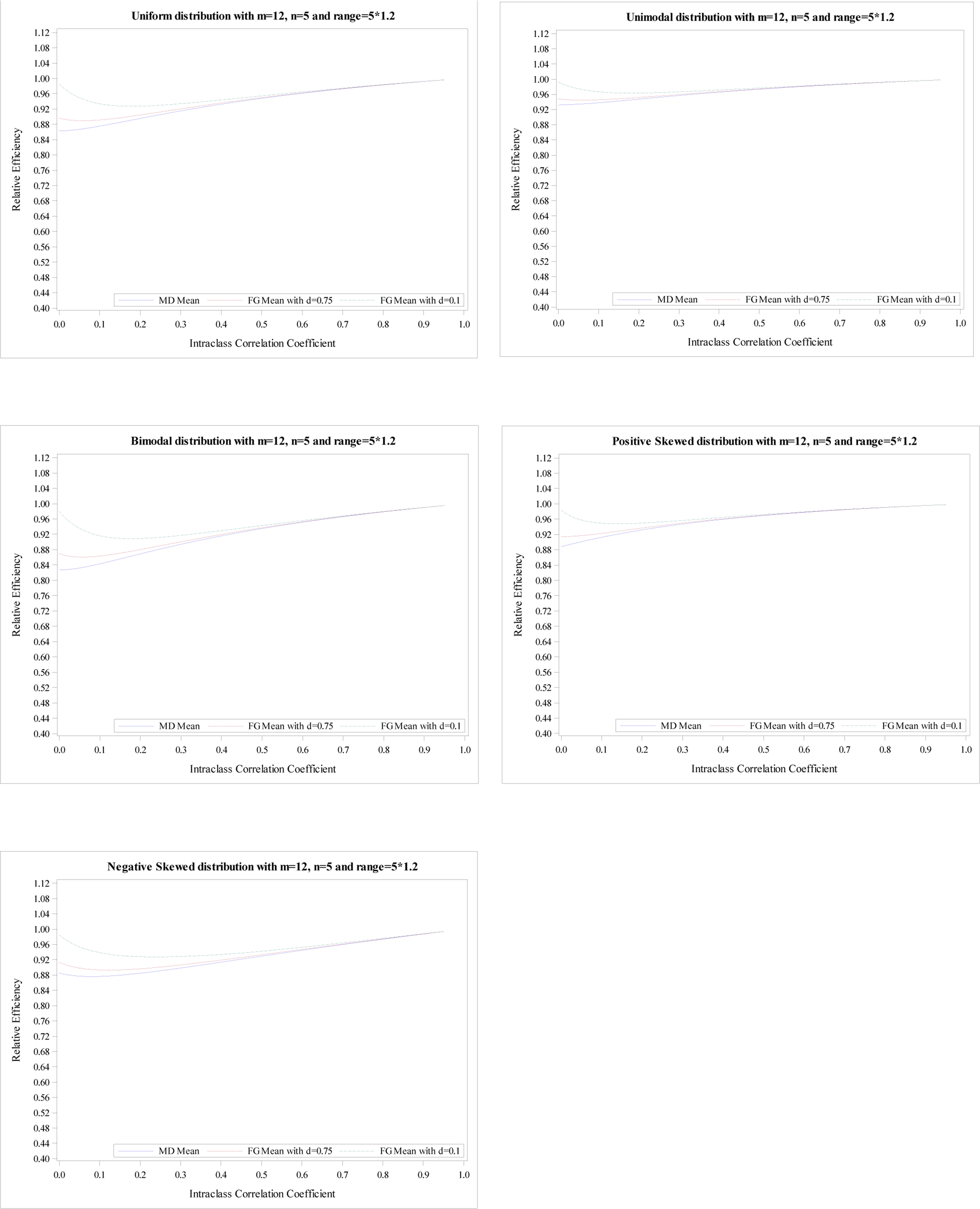
Relative efficiency of the treatment effect for five distributions with

m = 12, n = 5 and R = 5 × 1.2.

The mean RE from FG-corrected estimators with d = 0.1 decreases until the minimum is reached and then increases. Its maximum is obtained at ρ = 1 for all five distributions. Simultaneously, the mean RE from FG-corrected estimators with d = 0.75 have a similar pattern. However, the mean RE at ρ = 0 is much smaller than that from FG-corrected estimators with d = 0.1 but larger than the MD-corrected estimator. The mean REs from three estimators are pretty close when ρ > 0.1. Similar conclusions are shown in Figures 2–4. However, the RE’s differences at ρ = 0 among three estimators are more obvious when the range is higher. Additionally, for R = 1.2n, the mean REs from three estimators are very close when ρ > 0.2; For R = 1.6n, the mean REs from three estimators are very close when ρ > 0.3; For R = 1.8n, the mean REs from three estimators are very close when ρ > 0.4.

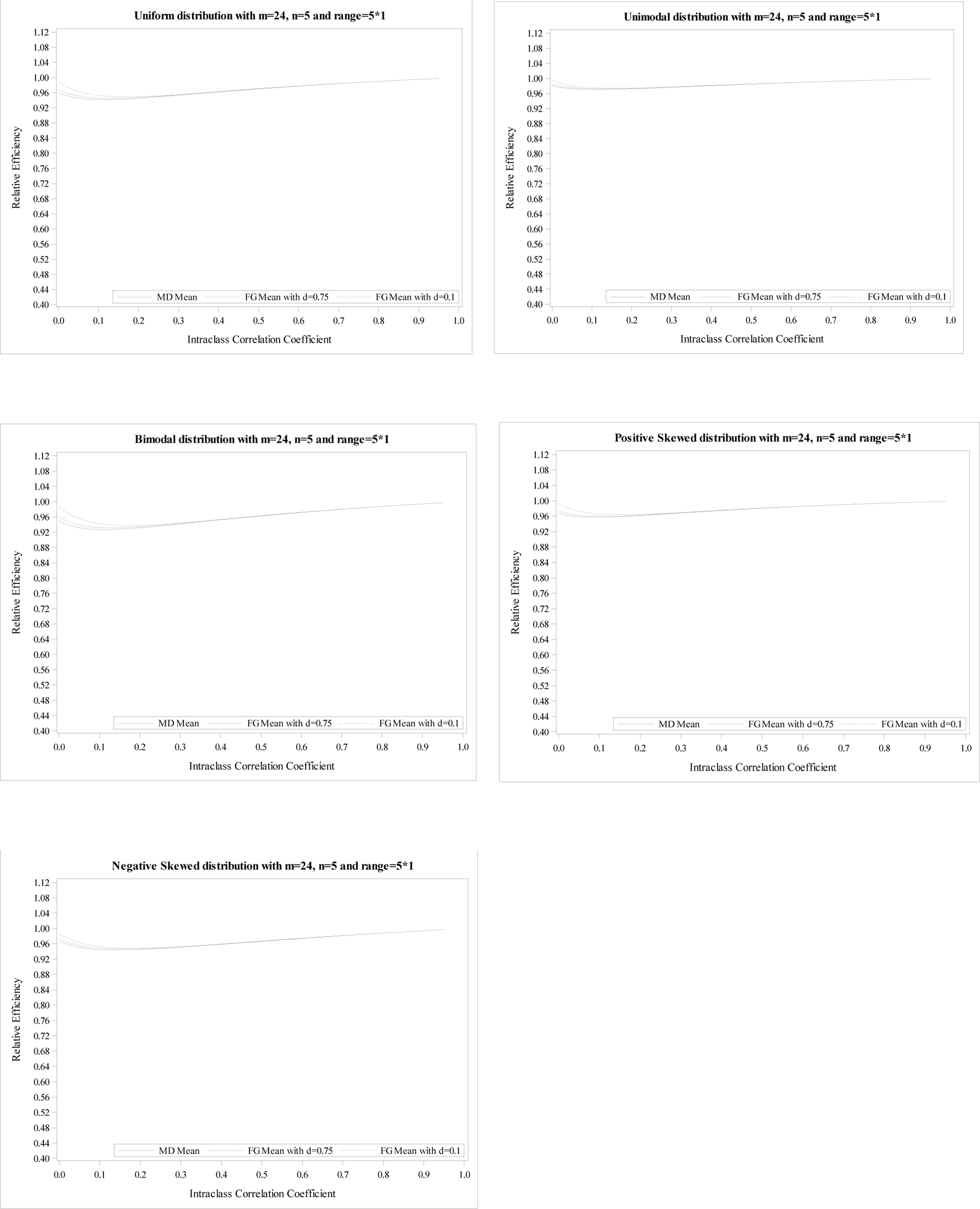
The plots of the mean RE based on simulation data with m = 24 and n = 5 for five distributions illustrate the same conclusions, shown in Appendix Figures 1–4. The minimums of mean REs from the 3 estimators (an MD-corrected estimator, FG-corrected estimators with d = 0.1 and d = 0.75) for R = n are above 93%, 94%, 93%, respectively. The minimum and maximum of minimum of mean RE across five distributions for all three estimators are 0.93 and 0.97. Additionally, the minimums are reached at ρ ∈ [0, 0.04]. For the range R = 1.2n, the minimum and maximum of minimum of mean RE across five distributions for all three estimators are 0.89 and 0.96. When the range increases to R = 1.8n, the smallest RE is 0.70 from MD-corrected estimator and a bimodal distribution.

When the cluster size n increases to 30, 60 and 120, we notice similar findings to when n = 5. These results can be provided per request. Since RE is defined as a ratio of equal versus unequal cluster size, e.g., n,n_i, the cluster size n plays little effect on the value of RE. That is, given a fixed number of cluster, REs do not vary much even if we increase cluster size manyfold. In summary, the mean REs are dependent on which bias-corrected estimator is considered, the number of clusters, and the CV value. For CRTs with a small number of clusters, e.g. ≤ 20, the mean RE estimated from an MD-corrected estimator, FG-corrected estimators with d = 0.1 and d = 0.75 are in the range of 80%-90% if CV ≤ 0.5; the mean RE estimated from an MD-corrected estimator, FG-corrected estimators with d = 0.1 and d = 0.75 are as low as 58% if CV>0.5. For CRTs with a small number of clusters, e.g. >20 but ≤40, the mean RE estimated from an MD-corrected estimator, FG-corrected estimators with d = 0.1 and d = 0.75 are close to 90% if CV ≤0.5; the mean RE estimated from an MD-corrected estimator, FG-corrected estimators with d = 0.1 and d = 0.75 are around 70% if CV>0.5. The simulation results are summarized in the top section -“Known CV” in the proposed diagram.

Appendix Tables 3–4 show the minimum of mean REs under five distributions for continuous and count outcomes with β₁ = 1.5. The mean REs estimated from an MD-corrected estimator and FG-corrected estimators with d = 0.1 and d = 0.75 for both types of outcomes have the similar results compared with those in Table 2. Even if we set the different values of p₀ and p₁ in the binary outcome and of β₁ in the count outcome, the findings remain consistent across the simulation settings.

4. Proposed algorithm

Section 3 shows that RE could be decreased to 58% under certain scenarios and REs do not vary much even if cluster size increases for a fixed number of clusters. Thus, we should increase the number of clusters in order to compensate for efficiency loss due to unequal cluster sizes. The distribution of cluster sizes and its range in a real world setting might be unknown. Therefore, for simplicity and to be conservative, we propose an algorithm to approximate RE based on our simulation results. If CV is unknown, then the RE from CV>0.5 is chosen. If CV is not provided but the range of CV is available, we suggest using the maximum of CV in the proposed algorithm. As shown in our proposed algorithm, we find that there are little RE differences between m = 12 and m = 24 for an FG-corrected estimator with d = 0.1. An FG-corrected estimator with d = 0.75 is often used in the analysis but REs have some differences depending on the different number of clusters. Thus, we suggest using the same bias-corrected estimator in the sample size calculation at the design stage as in the subsequent data analysis.

For CRTs with few clusters and binary outcomes, Li and Redden (Li et al., 2015) proposed a specific power formula from the GEE model with an equal number of clusters per group and equal cluster sizes across all clusters,

$$power=1-T_{m-2}\left\{t_{1-\frac{\alpha }{2},m-2}-\frac{{\beta }_1\sqrt{m}}{\sqrt{\left(\frac{m}{m-2}\right)\left(\frac{1+\left(n-1\right)\rho }{n}\right)\left(\frac{2}{p_1(1-p_1)}+\frac{2}{p_0(1-p_0)}\right)}}\right\}.$$ (12)

Given the pre-determined type I error α, ρ and expected power, the cluster size n or the number of clusters m can be calculated from this equation, presuming either one is known. For example, ρ = 0.03, p₀ = 0.2, p₁ = 0.3, and m = 26, n = 140 is needed to reach 80% power at the type I error of 5%. If the cluster size n = 200 is known, m = 26 gives 82.4% power at the type I error of 5%.

Table 3 shows the comparisons for number of clusters for an unknown CV between our proposed approach and the available formulas. When ρ = 0.01 and n = 140, a minimal of estimated number of clusters m = 16 is needed to reach 80% power at the type I error of 5% from Equation (12). Given an unknown CV and m ≤ 20, our proposed algorithm shows RE=0.58 for an MD-corrected estimator, RE=0.75 for an FG-corrected estimator with d = 0.1 and RE=0.64 for an FG-corrected estimator with d = 0.75, respectively. Therefore, the number of clusters will be 16/0.58=27.6 for an MD-corrected estimator, 16/0.75=21.3, and 16/0.64=25 for an FG-corrected estimator with d = 0.1 and with d = 0.75, respectively. They will be rounded up to an even number for an equal location. On the other hand, Liu and Liang (Liu et al., 1997) calculated the number of clusters from asymptotic variance estimate. Liu and Colditz (Liu et al., 2018) derived RE based on the same asymptotic variance equation and they find that small CRTs (e.g., N = 200), medium CRTs (e.g., N = 600), and large CRTs (e.g., N = 2000) have 21%, 16%, and 14% efficiency loss when the number of clusters is small (m = 5, 6, 20). The calculated number of clusters from Liu and Liang (Liu et al., 1997) and adjusted number of clusters based on Liu and Colditz (Liu et al., 2018) are also included in Table 3, e.g., 10/0.84=11.9.

Table 3.

Number of clusters comparisons with unknown CV, p₀ = 0.2 and p₁ = 0.3

ρ	n	Bias-corrected				Asymptotic
		Li and Redden[1]	MD-corrected estimator[2]	FG-corrected estimator with d=0.1[2]	FG-corrected estimator with d=0.75[2]	Liu and Liang[1]	Liu and Colditz[3]
0.01	140	16	28	22	26	12	14
	200	14	26	20	24	10	12
	300, 400, 500, 1000	12	22	18	20	8	10
0.03	140, 200	26	38	36	38	22	26
	300, 400, 500, 1000	24	36	34	34	20	24

^[1]Assume equal cluster sizes;

^[2]Adjustment from the proposed algorithm due to unequal cluster sizes for finite clusters;

^[3]Adjustment from the algorithm due to unequal cluster sizes;

When comparing the number of clusters from Li and Redden (Li et al., 2015) and Liu and Liang (Liu et al., 1997) assuming equal cluster sizes, at least an additional 18% of clusters are needed because of bias-correction. When comparing REs presented in Section 3 and Liu and Colditz (Liu et al., 2018), the newly proposed strategy has more efficiency loss when CV is unknown. Finally, we need at least 38% more clusters to design a CRT with unequal cluster sizes, e.g, m = 36 from an FG-corrected estimator with d = 0.1 versus m = 26 from Liu and Colditz (Liu et al., 2018).

Further, Li and Redden (Li et al., 2015) make a correction allowing unequal cluster sizes by replacing $\frac{1+\left(n-1\right)\rho }{n}$ by $\frac{1+\left[\left({\mathrm{C}\mathrm{V}}^2\frac{m-1}{m}+1\right)n-1\right]\rho }{n}$ in Equation (12). Table 6 illustrates the estimated number of clusters given ρ, n, and CV. If assuming ρ = 0.01, n = 140, and CV=0.6, then an enrollment of m = 18 has 80% power. On the other hand, we obtain the needed number of clusters from our proposed algorithm. First, m = 16 using Equation (12). The proposed clusters from an MD-corrected estimator and FG-corrected estimators will be 16/0.58 = 27.6≈28, 16/0.75 = 21.3≈22, and 16/0.64 = 25≈26 using our proposed algorithm. As shown in Table 4, the number of clusters using known CV from Li and Redden⁴² does not change much even if CVs vary from 0.1 to 0.6.

Table 4.

Number of clusters comparisons with known CV, p₀ = 0.2 and p₁ = 0.3

ρ	n	CV	Li and Redden[1]	MD-corrected estimator[2]	FG-corrected estimator with d=0.1[2]	FG-corrected estimator with d=0.75[2]
0.01	140	0.1–0.4	16	20	18	20
		0.5	16	28	22	26
		0.6	18
	200	0.1–0.4	14	18	16	18
		0.5–0.6	16	26	20	24
0.03	140	0.1–0.3	28	30	30	30
		0.4	30
		0.5	32	38	36	38
		0.6	34
	200	0.1–0.2	26	30	30	30
		0.3–0.4	28
		0.5	30	38	36	38
		0.6	32

^[1]Assume unequal cluster sizes;

^[2]Adjustment from the proposed algorithm due to unequal cluster sizes for finite clusters;

To our knowledge, no sample size formulas based on GEE models assuming equal cluster sizes with a small number of clusters are available for continuous and count outcomes. We still use Equation (6) in Shih (Shih, 1997) for continuous outcomes and formula (3) (Amatya et al., 2013) for count data, the cluster size n or the number of clusters m can be calculated from these equations if either one is known. Then, we increase the number of clusters accounting for efficiency loss from our proposed algorithm.

5. A Real World Example

The Dominantly Inherited Alzheimer Network (DIAN) observational study enrolls biological adult children of a parent with a mutated gene (Presenilin1, Presenilin2 or APP), which is known to cause dominantly inherited Alzheimer’s disease (DIAD). One of the major goals in establishing the DIAN by the funding agency (i.e., the National Institute of Health) is to facilitate future prevention or therapeutic trials on DIAD. Because multiple family members from the same families are enrolled in the DIAN, one possibility is to implement future clinical trials in the DIAN using a CRT design with families as the clusters. If such a CRT will be implemented, the nature of these rare mutations implies that the number of clusters will not be large. Further, the family size in the DIAN varies from 1 to 10+. Therefore, the design of a future CRT in the DIAN must take into account both a small number of families and very different unequal family sizes.

We consider a two-arm trial in which one active treatment is tested against the placebo in slowing the cognitive decline. We are interested in a cognitive composite which combines four measures of episodic memory, executive functioning, processing speed, and mental status. Wang et al detailed the assessments of these measures and how to construct a single composite (Wang et al., 2018). Briefly, this cognitive composite is a weighted sum of z-scores, using mean and standard deviation from healthy participants. We aim to test the difference in the annual rate of change for this cognitive composite for the mutation carriers between intervention and placebo.

Our preliminary data for symptomatic subjects shows the mean and standard deviation of annual change from baseline of the cognitive composite in the DIAN database is -0.217±0.165. The ICC of the cognitive composite across the families is 0.38. Using these data as the symptomatic subjects for the placebo arm of a future CRT on the DIAN, to test a reduction of 38% in the active treatment with the assumptions of an equal family size of 3, we found that 19 families per arm (m=38) are needed to reach 80% power at the two-sided significance level using the explicit formula for continuous outcome (Liu et al., 1997). Because of the very unequal family sizes in the DIAN which implies that the CV of family size in the DIAN study is very large (>0.5), to account for the efficiency loss, we will have to enroll 28, 26, and 27 families per arm if using MD-corrected estimator, an FG-corrected estimator with d=0.1 and with d=0.75, based on our proposed algorithm when the family size varies. These numbers are about 1/3 higher than the 19 families needed when family size is equal.

6. Discussion

In this paper, we derived REs for estimating treatment effect in CRTs with equal versus unequal cluster sizes when only a small number of clusters are available. Our approaches were based on two bias-corrected sandwich estimators and can be applied to three common types of efficacy outcomes. First, unlike the RE formula as derived in Liu and Colditz (Liu et al., 2018), RE’s formulas are different for continuous, binary, and count data using bias-corrected sandwich estimators. They also depend on the cluster allocations π and the treatment effect βM₁. However, we noticed little RE differences when different values of β₁ were considered in the simulation studies. Second, different boundaries in F-G bias-estimators produced different REs. Specifically, the boundary d = 0.1 always had a larger RE than d = 0.75. We found that there were little RE differences between m = 12 and m = 24 for a FG-corrected estimator with d = 0.1 while REs for a FG-corrected estimator with d = 0.75 had some differences for the different number of clusters. Thus, in the subsequent data analysis, we suggested using the same bias-corrected estimator that is used in the sample size calculation. Third, REs varied little even if cluster size increases for a fixed number of clusters. Instead, the number of clusters should be increased in order to compensate for efficiency loss due to unequal cluster sizes. Therefore, we provided a guide for practical use to increase the number of clusters when unequal cluster size occurs. Fourth, unlike the formula proposed by Li and Redden (Li et al., 2015), where the exact value of CV is required, our proposed algorithm work for unknown CV, known CV or range of CV. Lastly, Van Breukelen et al (Van Breukelen et al., 2007) concluded that the loss of efficiency due to variation of cluster sizes rarely exceeds 10 percent and could be larger than 10% when CV exceeds 0.63. However, we found that the number of clusters could be increased by as much as 18% when CV < 0.5 and 42% when CV ≥ 0.5.

When a CRT with a small number of clusters is expected, researchers intend to increase the cluster size to reach the desired power. However, the third column of Table 3 shows that the number of clusters are kept the same to reach 80% power for ρ = 0.01 at the type I error of 5% using Equation (12), even if the cluster size increases from 300 to 1000. Researchers (Lui, 1991; Frison et al., 1992; Lui et al., 1992) also demonstrated that increasing the number of measurements in longitudinal studies has limited effect on the power. The conclusion also applies to CRTs – sometimes it is almost impossible to obtain the desired power unless more clusters are enrolled. On the other hand, when the increase of the number of clusters is possible, we can decrease the cluster size and smaller total sample size to obtain the same power. For example, an equal cluster size of 300 and 12 clusters can obtain 80% power using Equation (12); a cluster size of 140 with CV=0.4 and 20 clusters from an MD-corrected estimator can obtain 80% power from our proposed algorithm. As seen, the total sample size from our proposed algorithm, e.g., 2800, is much less than 3600. We demonstrated our proposed methodology by applying it to design a future CRT on the DIAN in which families serve as the cluster, and found that, to compensate for the efficacy loss due to very skewed distribution of family sizes, the number of families may have to increase by 1/3 to achieve the same statistical power for detecting the same effect size, in comparison to the number of families needed under the assumption of identical family size.

Finally, the sample size formulas including covariates in the GEE model are definitely more complicated than those in sections 2. Liu and Liang also showed that the performance of the sample size formula is sensitive to the distribution of the covariates (Liu et al., 1997). Therefore, our research does not consider the covariates in the sample size calculation.

Figure 3.

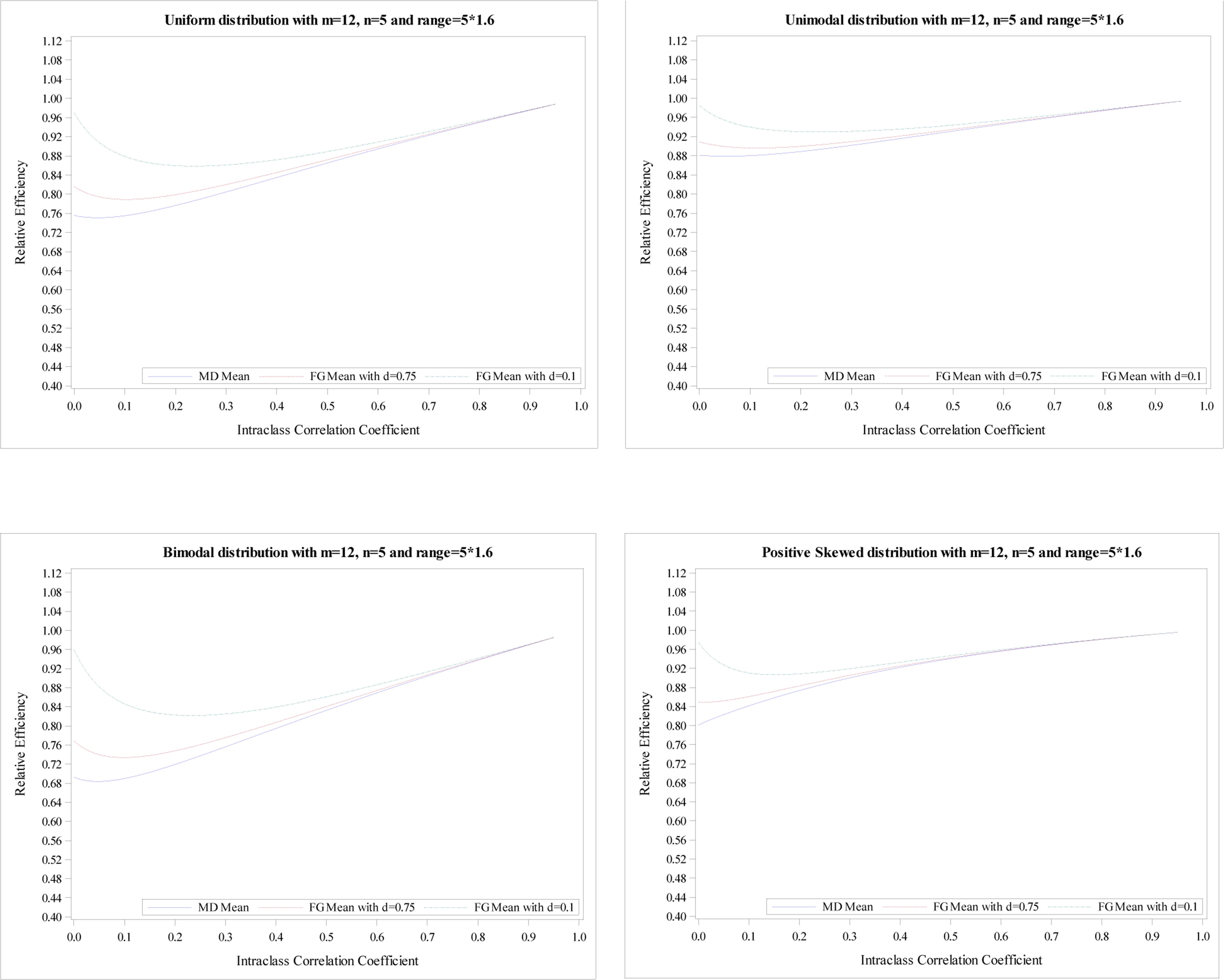
Relative efficiency of the treatment effect for five distributions with

m = 12, n = 5 and R = 5 × 1.6.

Appendix

Figure 1.

Relative efficiency of the treatment effect for five distributions with

m = 24, n = 5 and R = 5.

Figure 2.

Relative efficiency of the treatment effect for five distributions with

m = 24, n = 5 and R = 5 × 1.2.

Figure 3.

Relative efficiency of the treatment effect for five distributions with

m = 24, n = 5 and R = 5 × 1.6.

Figure 4.

Relative efficiency of the treatment effect for five distributions with

m = 24, n = 5 and R = 5 × 1.8.

Appendix Table 1.

Cluster size distributions

Distribution	Cluster frequencies	Cluster sizes
Uniform	$f_a=f_b=f_c=\frac{m}{3}$	$g_a=n-\frac{R}{2}$	gb = n	$g_c=n+\frac{R}{2}$
Unimodal	$f_a=\frac{m}{6},$ $f_b=\frac{2m}{3},$ $f_c=\frac{m}{6}$	$g_a=n-\frac{R}{2}$	gb = n	$g_c=n+\frac{R}{2}$
Bimodal	$f_a=\frac{5m}{12},$ $f_b=\frac{m}{6},$ $f_c=\frac{5m}{12}$	$g_a=n-\frac{R}{2}$	gb = n	$g_c=n+\frac{R}{2}$
Positively Skewed	$f_a=\frac{m}{2},$ $f_b=\frac{m}{3},$ $f_c=\frac{m}{6}$	$g_a=n-\frac{R}{3}$	$g_b=n+\frac{R}{6}$	$g_c=n+\frac{2R}{3}$
Negatively Skewed	$f_a=\frac{m}{6},$ $f_b=\frac{m}{3},$ $f_c=\frac{m}{2}$	$g_a=n-\frac{2R}{3}$	$g_b=n-\frac{R}{6}$	$g_c=n+\frac{R}{3}$

m = # of clusters; n = cluster sizes;

f_a = # of clusters with cluster size g_a; f_b = # of clusters with cluster size g_b; f_c = # of clusters with cluster size g_c;

R = range of cluster sizes = g_c − g_a.

Appendix Table 2.

Coefficient of variation (CV) of cluster size

Cluster sizes n	# of clusters m	Range R	CV
			Uniform	Unimodal	Bimodal	Positively Skewed	Negatively Skewed
5/30/60/120	12	n	0.43	0.30	0.48	0.39	0.39
		1.2n	0.51	0.36	0.57	0.47	0.47
		1.6n	0.68	0.48	0.76	0.62
		1.8n	0.77	0.54	0.86	0.70
	24	n	0.42	0.29	0.47	0.38	0.38
		1.2n	0.50	0.35	0.56	0.46	0.46
		1.6n	0.67	0.47	0.75	0.61
		1.8n	0.75	0.53	0.84	0.69

Shading: Not applicable (g_a < 0)

Appendix Table 3.

Minimum of mean RE for the different simulation designs with continuous outcomes

Cluster sizes n	# of clusters m	Range R	Distribution	ρ, Minimum[2] of mean RE[1]
				MD-corrected estimator	FG-corrected estimator
					d=0.1	d=0.75
5	12	n	Uniform	0, 0.91	0.16, 0.95	0.05, 0.93
			Unimodal	0, 0.95	0.16, 0.98	0.06, 0.96
			Bimodal	0, 0.88	0.16, 0.94	0.05, 0.91
			Positive Skewed	0, 0.92	0.14, 0.96	0.02, 0.94
			Negative Skewed	0.05, 0.92	0.21, 0.95	0.09, 0.93
		1.2n	Uniform	0, 0.86	0.18, 0.93	0.06, 0.89
			Unimodal	0, 0.93	0.18, 0.96	0.17, 0.95
			Bimodal	0.01, 0.83	0.18, 0.91	0.06, 0.86
			Positive Skewed	0, 0.89	0.14, 0.95	0.02, 0.92
			Negative Skewed	0.08, 0.88	0.24, 0.93	0.13, 0.90
		1.6n	Uniform	0.05, 0.75	0.23, 0.86	0.11, 0.79
			Unimodal	0.06, 0.88	0.23, 0.93	0.12, 0.90
			Bimodal	0.05, 0.69	0.23, 0.82	0.11, 0.74
			Positive Skewed	0, 0.80	0.15, 0.91	0.02, 0.85
		1.8n	Uniform	0.11, 0.67	0.28, 0.80	0.17, 0.72
			Unimodal	0.13, 0.84	0.28, 0.90	0.19, 0.86
			Bimodal	0.11, 0.59	0.28, 0.75	0.16, 0.65
			Positive Skewed	0, 0.75	0.16, 0.88	0.03, 0.82
	24	n	Uniform	0.11, 0.94	0.17, 0.95	0.13, 0.95
			Unimodal	0.11, 0.97	0.17, 0.97	0.13, 0.97
			Bimodal	0.11, 0.93	0.18, 0.94	0.13, 0.93
			Positive Skewed	0.09, 0.96	0.15, 0.96	0.11, 0.96
			Negative Skewed	0.14, 0.94	0.19, 0.95	0.16, 0.95
		1.2n	Uniform	0.12, 0.91	0.19, 0.93	0.14, 0.92
			Unimodal	0.13, 0.96	0.18, 0.96	0.14, 0.96
			Bimodal	0.12, 0.89	0.19, 0.91	0.14, 0.90
			Positive Skewed	0.09, 0.94	0.16, 0.95	0.11, 0.94
			Negative Skewed	0.18, 0.91	0.23, 0.92	0.20, 0.92
		1.6n	Uniform	0.17, 0.83	0.23, 0.85	0.19, 0.84
			Unimodal	0.17, 0.91	0.23, 0.92	0.19, 0.92
			Bimodal	0.16, 0.79	0.23, 0.82	0.18, 0.80
			Positive Skewed	0.10, 0.89	0.17, 0.91	0.12, 0.90
		1.8n	Uniform	0.23, 0.76	0.29, 0.79	0.25, 0.77
			Unimodal	0.24, 0.88	0.29, 0.89	0.25, 0.89
			Bimodal	0.22, 0.70	0.29, 0.75	0.24, 0.72
			Positive Skewed	0.10, 0.86	0.17, 0.88	0.12, 0.87

^[1]The mean RE among 1000 simulations is calculated for each ρ.

^[2]The minimum of mean RE including the corresponding ρ is identified across all the values of ρ.

Appendix Table 4.

Minimum of mean RE for the different simulation designs with β₁ = 1.5

Cluster sizes n	# of clusters m	Range R	Distribution	ρ, Minimum[2] of mean RE[1]
				MD-corrected estimator	FG-corrected estimator
					d=0.1	d=0.75
5	12	n	Uniform	0.01, 0.91	0.17, 0.95	0.02, 0.92
			Unimodal	0, 0.96	0.17, 0.98	0.03, 0.96
			Bimodal	0.01, 0.89	0.17, 0.94	0.03, 0.90
			Positive Skewed	0, 0.93	0.15, 0.97	0, 0.93
			Negative Skewed	0.06, 0.92	0.22, 0.95	0.07, 0.92
		1.2n	Uniform	0.02, 0.87	0.19, 0.93	0.04, 0.88
			Unimodal	0.02, 0.94	0.19, 0.96	0.04, 0.94
			Bimodal	0.04, 0.84	0.19, 0.91	0.04, 0.85
			Positive Skewed	0, 0.90	0.15, 0.95	0, 0.90
			Negative Skewed	0.10, 0.88	0.25, 0.93	0.11, 0.89
		1.6n	Uniform	0.07, 0.76	0.25, 0.86	0.09, 0.77
			Unimodal	0.08, 0.88	0.25, 0.93	0.10, 0.89
			Bimodal	0.07, 0.70	0.25, 0.83	0.09, 0.72
			Positive Skewed	0, 0.82	0.16, 0.91	0, 0.83
		1.8n	Uniform	0.13, 0.69	0.30, 0.81	0.15, 0.70
			Unimodal	0.15, 0.84	0.30, 0.90	0.17, 0.85
			Bimodal	0.12, 0.60	0.30, 0.76	0.14, 0.62
			Positive Skewed	0, 0.77	0.18, 0.89	0, 0.79
	24	n	Uniform	0.12, 0.94	0.18, 0.95	0.12, 0.94
			Unimodal	0.12, 0.97	0.17, 0.97	0.12, 0.97
			Bimodal	0.12, 0.93	0.18, 0.94	0.12, 0.93
			Positive Skewed	0.09, 0.96	0.16, 0.96	0.10, 0.96
			Negative Skewed	0.15, 0.95	0.19, 0.95	0.15, 0.95
		1.2n	Uniform	0.13, 0.92	0.19, 0.93	0.13, 0.92
			Unimodal	0.13, 0.96	0.18, 0.96	0.14, 0.96
			Bimodal	0.13, 0.89	0.19, 0.91	0.13, 0.90
			Positive Skewed	0.10, 0.94	0.16, 0.95	0.10, 0.94
			Negative Skewed	0.19, 0.91	0.23, 0.92	0.19, 0.92
		1.6n	Uniform	0.18, 0.83	0.23, 0.85	0.18, 0.84
			Unimodal	0.18, 0.92	0.23, 0.92	0.18, 0.92
			Bimodal	0.17, 0.79	0.23, 0.82	0.18, 0.79
			Positive Skewed	0.10, 0.89	0.17, 0.91	0.11, 0.89
		1.8n	Uniform	0.24, 0.77	0.29, 0.79	0.24, 0.77
			Unimodal	0.24, 0.88	0.29, 0.89	0.25, 0.89
			Bimodal	0.23, 0.71	0.29, 0.75	0.24, 0.71
			Positive Skewed	0.11, 0.86	0.18, 0.88	0.11, 0.86

^[1]The mean RE among 1000 simulations is calculated for each ρ.

^[2]The minimum of mean RE including the corresponding ρ is identified across all the values of ρ.

References

- Amatya A, Bhaumik D and Gibbons R (2013). Sample size determination for clustered count data. Statistics in Medicine 32:4162–4179. [DOI] [PMC free article] [PubMed] [Google Scholar]
- Austin P (2007). A comparison of the statistical power of different methods for the analysis of cluster randomization trials with binary outcomes. Statistics in Medicine 26:3550–3565. [DOI] [PubMed] [Google Scholar]
- Candel MJJM and Van Breukelen GJP (2010). Sample size adjustments for varying cluster sizes in cluster randomized trials with binary outcomes analyzed with second-order PQL mixed logistic regression. Statistics in Medicine 29(14):1488–1501. [DOI] [PubMed] [Google Scholar]
- Candel MJJM, Van Breukelen GJP, Kotova L and Berger MPF (2008). Optimality of Equal vs. Unequal Cluster Sizes in Multilevel Intervention Studies: A Monte Carlo Study for Small Sample Sizes. Communications in Statistics - Simulation and Computation 37(1):222–239. [Google Scholar]
- Donner A, Birkett N and Buck C (1981). Randomization by cluster-sample size requirements and analysis. American Journal of Epidemiology 114:906–914. [DOI] [PubMed] [Google Scholar]
- Eldridge S, Ashby D and Kerry S (2006). Sample size for cluster randomized trials: effect of coefficient of variation of cluster size and analysis method. International Journal of Epidemiology 35:1292–1300. [DOI] [PubMed] [Google Scholar]
- Emrich LJ and Piedmonte MR (1992). On some small sample properties of generalized estimating equationEstimates for multivariate dichotomous outcomes. Journal of Statistical Computation and Simulation 41(1–2):19–29. [Google Scholar]
- Fay MP and Graubard BI (2001). Small-sample adjustments for Wald-type tests using sandwich estimators. Biometrics 57(4):1198–1206. [DOI] [PubMed] [Google Scholar]
- Feng Z, McLerran D and Grizzle J (1996). A comparison of statistical methods for clustered data analysis with Gaussian error. Statistics in medicine 15(16):1793–1806. [DOI] [PubMed] [Google Scholar]
- Frison L and Pocock SJ (1992). Repeated measures in clinical trials: analysis using mean summary statistics and its implications for design. Statistics in medicine 11(13):1685–1704. [DOI] [PubMed] [Google Scholar]
- Gunsolley JC, Getchell C and Chinchilli VM (1995). Small sample characteristics of generalized estimating equations. Communications in Statistics - Simulation and Computation 24(4):869–878. [Google Scholar]
- Kauermann G and Carroll RJ (2001). A Note on the Efficiency of Sandwich Covariance Matrix Estimation. Journal of the American Statistical Association 96(456):1387–1396. [Google Scholar]
- Li P and Redden DT (2015). Small sample performance of bias-corrected sandwich estimators for cluster-randomized trials with binary outcomes. Statistics in Medicine 34(2):281–296. [DOI] [PMC free article] [PubMed] [Google Scholar]
- Liang K-Y and Zeger SL (1986). Longitudinal Data Analysis Using Generalized Linear Models. Biometrika 73(1):13–22. [Google Scholar]
- Liu G and Liang K-Y (1997). Sample Size Calculations for Studies with Correlated Observations. Biometrics 53(3):937–947. [PubMed] [Google Scholar]
- Liu J and Colditz GA (2018). Relative efficiency of unequal versus equal cluster sizes in cluster randomized trials using generalized estimating equation models. Biometrical journal. Biometrische Zeitschrift 60(3):616–638. [DOI] [PMC free article] [PubMed] [Google Scholar]
- Liu J and Colditz GA (R & R). Sample size calculation in three-level cluster randomized trials using generalized estimating equation models. [DOI] [PMC free article] [PubMed] [Google Scholar]
- Lui K-J (1991). Sample sizes for repeated measurements in dichotomous data. Statistics in Medicine 10(3):463–472. [DOI] [PubMed] [Google Scholar]
- Lui K-J and Cumberland WG (1992). Sample size requirement for repeated measurements in continuous data. Statistics in Medicine 11(5):633–641. [DOI] [PubMed] [Google Scholar]
- Manatunga AK, Hudgens MG and Chen S (2001). Sample Size Estimation in Cluster Randomized Studies with Varying Cluster Size. Biometrical Journal 43(1):75–86. [Google Scholar]
- Mancl LA and DeRouen TA (2001). A covariance estimator for GEE with improved small-sample properties. Biometrics 57(1):126–134. [DOI] [PubMed] [Google Scholar]
- Morel JG, Bokossa MC and Neerchal NK (2003). Small Sample Correction for the Variance of GEE Estimators. Biometrical Journal 45(4):395–409. [Google Scholar]
- Murray DM, Varnell SP and Blitstein JL (2004). Design and analysis of group-randomized trials: a review of recent methodological developments. American journal of public health 94(3):423–432. [DOI] [PMC free article] [PubMed] [Google Scholar]
- O'Brien LM and Fitzmaurice GM (2004). Analysis of longitudinal multiple-source binary data using generalized estimating equations. Journal of the Royal Statistical Society: Series C (Applied Statistics) 53(1):177–193. [Google Scholar]
- Paik MC (1988). Repeated measurement analysis for nonnormal data in small samples. Communications in Statistics - Simulation and Computation 17(4):1155–1171. [Google Scholar]
- Rosner B and Glynn R (2011). Power and Sample size estimation for the clustered Wilcoxon test. Biometrics 67:646–653. [DOI] [PMC free article] [PubMed] [Google Scholar]
- Rosner B, Glynn R and Lee M (2003). Incorporation of clustering effects for the Wilcoxon rank sum test: a large-sample approach. Biometrics 59:1089–1098. [DOI] [PubMed] [Google Scholar]
- Shih WJ (1997). Sample Size and Power Calculations for Periodontal and Other Studies with Clustered Samples Using the Method of Generalized Estimating Equations. Biometrical Journal 39(8):899–908. [Google Scholar]
- Teerenstra S, Lu B, Preisser JS, van Achterberg T and Borm GF (2010). Sample size considerations for GEE analyses of three-level cluster randomized trials. Biometrics 66(4):1230–1237. [DOI] [PMC free article] [PubMed] [Google Scholar]
- Turner RM, Prevost AT and Thompson SG (2004). Allowing for imprecision of the intracluster correlation coefficient in the design of cluster randomized trials. Statistics in Medicine 23(8):1195–1214. [DOI] [PubMed] [Google Scholar]
- Van Breukelen GJ and Candel MJ (2012). Calculating sample sizes for cluster randomized trials: we can keep it simple and efficient! Journal of clinical epidemiology 65(11):1212–1218. [DOI] [PubMed] [Google Scholar]
- Van Breukelen GJ, Candel MJ and Berger MP (2008). Relative efficiency of unequal cluster sizes for variance component estimation in cluster randomized and multicentre trials. Statistical Methods in Medical Research 17(4):439–458. [DOI] [PubMed] [Google Scholar]
- Van Breukelen GJP, Candel MJJM and Berger MPF (2007). Relative efficiency of unequal versus equal cluster sizes in cluster randomized and multicentre trials. Statistics in Medicine 26(13):2589–2603. [DOI] [PubMed] [Google Scholar]
- Westgate PM and Burchett WW (2016). Improving power in small-sample longitudinal studies when using generalized estimating equations. Statistics in Medicine. [DOI] [PMC free article] [PubMed] [Google Scholar]