Abstract
Deep learning in k-space has demonstrated great potential for image reconstruction from undersampled k-space data in fast magnetic resonance imaging (MRI). However, existing deep learning-based image reconstruction methods typically apply weight-sharing convolutional neural networks (CNNs) to k-space data without taking into consideration the k-space data’s spatial frequency properties, leading to ineffective learning of the image reconstruction models. Moreover, complementary information of spatially adjacent slices is often ignored in existing deep learning methods. To overcome such limitations, we have developed a deep learning algorithm, referred to as adaptive convolutional neural networks for k-space data interpolation (ACNN-k-Space), which adopts a residual Encoder-Decoder network architecture to interpolate the undersampled k-space data by integrating spatially contiguous slices as multi-channel input, along with k-space data from multiple coils if available. The network is enhanced by self-attention layers to adaptively focus on k-space data at different spatial frequencies and channels. We have evaluated our method on two public datasets and compared it with state-of-the-art existing methods. Ablation studies and experimental results demonstrate that our method effectively reconstructs images from undersampled k-space data and achieves significantly better image reconstruction performance than current state-of-the-art techniques. Source code of the method is available at https://gitlab.com/qgpmztmf/acnn-k-space.
Keywords: Magnetic resonance imaging, k-space, Attention, Deep learning
Graphical Abstarct
Introduction
Deep learning has shown great potential for image reconstruction from undersampled k-space data in fast magnetic resonance imaging (MRI) (Knoll et al., 2020; Liang et al., 2020). A variety of deep learning methods have been developed to solve the image reconstruction problem, including model-driven (Abdullah et al., 2019; Aggarwal et al., 2019; Cheng et al., 2018; Hammernik et al., 2018; Huang et al., 2019; Qin et al., 2018; Schlemper et al., 2018; Sriram et al., 2020) and data-driven methods (Akçakaya et al., 2019; Han et al., 2020; Jin et al., 2017; Kim et al., 2019; Lee et al., 2018; Quan et al., 2018; Wang et al., 2020; Wang et al., 2016; Zhu et al., 2018). Unlike model-driven methods whose performance is hinged on their model capacity, data-driven methods directly learn a mapping between undersampled k-space data and reconstructed images (Zhu et al., 2018), or an interpolation in image domain (Jin et al., 2017; Lee et al., 2018; Quan et al., 2018; Wang et al., 2016), k-space (Akçakaya et al., 2019; Han et al., 2020; Kim et al., 2019; Wang et al., 2020), or both the image domain and the k-space (Eo et al., 2018; Souza et al., 2019). Particularly, fully connected neural networks have been used to learn the Fourier transform itself (Zhu et al., 2018). However, it is difficult to use such a method to reconstruct large size images due to huge memory requirements of fully connected neural networks. In contrast, convolutional neural networks (CNNs) with weight sharing are memory efficient and therefore have been widely adopted to learn to interpolate from undersampled k-space data for image reconstruction in conjunction with Fast Fourier transform (FFT) (Akçakaya et al., 2019; Han et al., 2020; Kim et al., 2019; Wang et al., 2020).
Since CNNs in k-space could be used to directly interpolate the missing k-space samples (Akçakaya et al., 2019; Han et al., 2020; Kim et al., 2019; Wang et al., 2020), it is reasonable to believe that they could perform better than their counterparts working in the image domain with the same network architecture. However, existing k-space deep learning methods directly adopt CNNs without taking into consideration characteristics of the k-space data. First, the samples at the central k-space region (low spatial frequencies) contain most of the information of image contrast, while the samples further away from the center (high spatial frequencies) contain information about the edges and boundaries of the image. Therefore, applying weight-sharing CNNs to the entire k-space data, as used in most existing k-space deep learning methods, ignores distinctive contributions of different spatial frequencies of the k-space data to the image reconstruction, potentially leading to ineffective learning of CNNs. Although a fixed weighting map can be adopted as a weighting layer to modulate the output of CNNs (Han et al., 2020), it would be more desirable to obtain a weighting map capable of adaptively adjusting the output of CNNs to better interpolate the missing k-space samples. Second, undersampled k-space data of spatially adjacent image slices may provide complementary information for image reconstruction. However, most existing deep learning methods typically learn interpolations for spatially adjacent image slices independently, ignoring their complementary information that could potentially improve image reconstruction. Third, in multi-coil MRI acquisition, k-space data from different coils are sensitive to different regions of the object but are often treated equally as multiple channels in existing k-space deep learning image reconstruction methods, which may degrade image reconstruction performance.
In order to overcome the aforementioned limitations, we have developed a novel k-space deep learning framework for image reconstruction from undersampled k-space data, referred to as adaptive convolutional neural networks for k-space data interpolation (ACNN-k-Space). Particularly, a residual Encoder-Decoder network architecture is adopted to interpolate the undersampled k-space data with CNNs enhanced by a self-attention layer (Hu et al., 2018), referred to as frequency-attention layer, which adaptively assigns weights to features learned by CNNs for k-space samples at different spatial frequencies. Moreover, instead of learning interpolations for spatially adjacent image slices independently, our method learns an interpolation for each image slice by integrating slices within its spatial neighborhood as a multi-channel input, along with k-space data from multiple coils if available, to the residual network. Since the image slices may contribute to the image reconstruction differently and data from different coils are sensitive to different regions of the object, we adopt another self-attention layer, referred to as channel-attention layer (Roy et al., 2018), to adaptively assign weights to features learned by CNNs for different channels. Similar to two recent methods that adopt channel-wise attention to modulate learned features in either k-space or image domain (Huang et al., 2019; Lee et al., 2020), the channel-attention layers are also applied to all learned features in addition to the input image slices. Together, the residual Encoder-Decoder network with frequency-attention and channel-attention layers learns an interpolation for undersampled k-space data and reconstructs an image in conjunction with inverse FFT (IFFT) in an end-to-end fashion. Moreover, the method is generally applicable to both k-space and image domain data. We have evaluated our method based on two publicly available datasets. Ablation studies and experimental results show that our method could effectively reconstruct images from undersampled k-space data and achieve better image reconstruction performance than existing state-of-the-art techniques.
Materials and methods
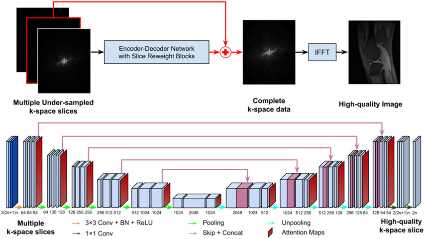
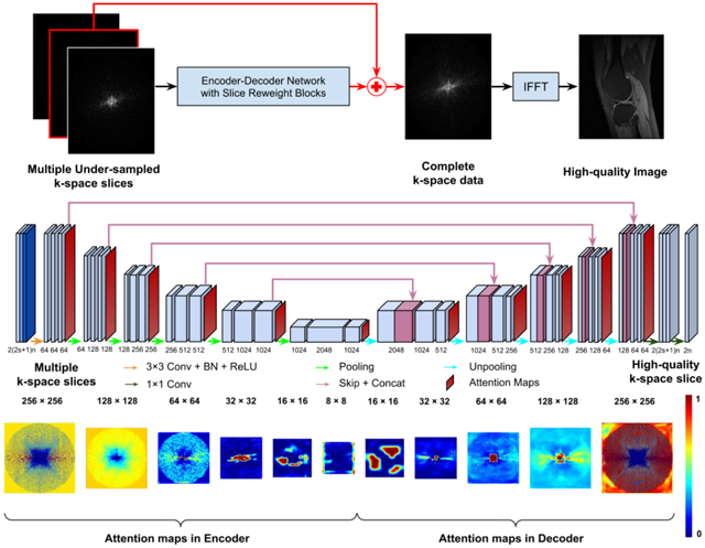
To generate missing k-space samples, we adopt a residual Encoder-Decoder network to reconstruct images from undersampled k-space data, as illustrated in Figure 1. The residual network learns an interpolation to reconstruct images in conjunction with IFFT from a multi-channel input that consists of undersampled k-space data from spatially adjacent slices and data from multiple coils if available. Its Encoder-Decoder component consists of CNNs, enhanced by frequency-attention and channel-attention layers. The network is optimized by minimizing a loss function L defined as the mean square error (MSE) between the reconstructed image and its corresponding image obtained from fully sampled k-space data:
| (1) |
where is the reconstructed image and is the image obtained from fully sampled k-space data of the j-th coil, and n is the number of coils.
Figure 1.
A residual Encoder-Decoder network of CNNs, enhanced by frequency-attention and channel-attention layers, for image reconstruction from undersampled k-space data. The residual network (top row) learns an interpolation to reconstruct images in conjunction with IFFT from a multi-channel input that consists of undersampled k-space data from spatially adjacent slices and data from multiple coils if available. Its Encoder-Decoder component (bottom row) consists of multiple layers of CNNs, enhanced by frequency-attention and channel-attention layers. Attention maps are the outputs of the frequency-attention and channel-attention layers to modulate features learned by CNNs before every pooling or unpooling layer.
A. Encoder-Decoder network architecture
We adopt an Encoder-Decoder network to learn an interpolation to generate missing k-space samples for image reconstruction from undersampled k-space data. As illustrated in Figure 1, the network backbone is a U-Net (Ronneberger et al., 2015), consisting of convolutional layers, followed by rectified linear unit (ReLU) (Agarap, 2018) and batch normalization (BN) (Ioffe and Szegedy, 2015), with parameters specified in Figure 1 (bottom).
For image reconstruction of each slice from its undersampled k-space data, the network’s input consists of complex valued k-space data of c = 2s + 1 slices within its spatial neighborhood, where s ≥ 0 is the consecutive slices stacked on top and bottom of the slice under consideration. Complex values of the k-space data are split into two channels of real value signals. For imaging data with multiple coils, k-space data of n coils are stacked as multi-channel data with each coil’s data as two channels of real value signals. Therefore, the number of channels of the input is 2(2s + 1 )n and the number of channels of the output is 2n to form complex valued k-space data. For a slice with fewer than s bottom or top slices, the data volume is padded with the first one adjacent to the current slice.
In order to take into consideration distinctive contributions of different spatial frequencies and different channels to the image reconstruction, we adopt self-attention layers to enhance the learning of CNNs.
B. Attention layers
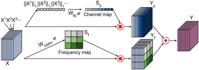
We adopt frequency-attention and channel-attention layers to enhance k-space deep learning. Both frequency-attention and channel-attention layers learn self-attention maps from their feature maps (Hu et al., 2018; Roy et al., 2018) to modulate features learned by CNNs and the modulated feature maps are aggregated by an element-wise Max-out operation, as illustrated in Figure 2.
Figure 2.
Self-attention layers learn a frequency-attention map (bottom) and a channel-attention map (top) respectively, and weighted feature maps are aggregated by an element-wise Max-out operation. Xi refers to the ith channel of the k-space feature maps, Yc refers to features weighted by the channel-attention map, Yf refers to features weighted by the frequency-attention map, and Y refers to the aggregated features of Yc and Yf through a Max-out operation.
B.1. Frequency-attention layers
The k-space samples are in the spatial frequency domain, and the samples at low frequencies characterize most of the signal intensity and contrast information of the image, while the samples at high frequencies characterize information about objects’ edges and boundaries. Existing k-space deep learning methods directly apply the weight-sharing CNNs to entire k-space data, ignoring distinct contributions of different frequencies of the k-space data to image reconstruction. To tackle this issue, we adopt a frequency-attention layer to modulate features learned by CNNs at different spatial frequencies. As illustrated in Figure 2 (bottom), given a k-space feature map X = {x{1,1}, x{1,2}, … , x{i,j}}, where corresponds to channel C and spatial location (i, j) with i ∈ [1, …, W] and j ∈ [1, …, H], W and H are width and height of a channel of k-space feature maps. The frequency-attention map is learned with a convolutional operation ⊛:
| (2) |
where is convolutional weights to be learned and σ is the sigmoid function. Each of the frequency-attention map represents the linearly combined representation of all channels for a spatial location (i, j). Then the input feature map X = {X1, … , Xi} is modulated by this frequency attention map Sf to generate frequency-attention weighted features Yf = SfX.
B.2. Channel-attention layers
Since spatially adjacent slices may provide complementary information to one another and data from different coils contribute differently to the image reconstruction, we integrate multiple slices and data from multiple coils as a multi-channel input to the network. Instead of treating them equally, we adaptively learn weights for them using a channel-attention layer. Given k-space feature maps of multiple slices X = {X1, X2, … , Xm}, where m is the number of channels in X, we employ a simple gating mechanism with a sigmoid activation to learn a channel-attention map:
| (3) |
where is parameters of a fully connect layer to be learned, σ is the sigmoid function, and ∥.∥1 is used to squeeze each Xi to yield a scalar value. Then the feature maps X = {X1, … , Xi} are modulated by this channel attention map Sc along the channel dimension to generate weighted features Yc = ScX.
We use an element-wise Max-out operator to aggregate the weighted features obtained by the frequency-attention and the channel-attention layers:
| (4) |
where Yc is the weighted features obtained by the channel-attention layers and Yf is the weighted features obtained by the frequency-attention layers. Both frequency-attention and channel-attention feature maps are learned with the entire network in an end-to-end learning fashion by minimizing the loss function.
C. Evaluation and ablation studies
C.1. Datasets
We evaluated our method on two publicly available datasets, including Stanford Fully Sampled 3D FSE Knee k-space Dataset (available at http://mridata.org/), and fastMRI Brain Dataset (Zbontar et al., 2018) (available at https://fastmri.org). Stanford dataset contains 20 cases of knee images, collected with 8 coils. Each image is a 3D volume with 256 slices. We randomly selected 15 cases as training data, one case as validation data, and the remaining four cases as test data. fastMRI dataset contains 4,478 cases, collected with 8, 12, 16, 20 or 24 coils. For the convenience of network training, we selected 570 cases collected with 16 coils from the dataset. Each case is a 3D volume with 16 slices. All images from this dataset were zero-padded to have the same size of 640 × 320. We randomly selected 500 cases as training data, 10 as validation data, and the remaining 60 as test data.
The input k-space was undersampled using two different sampling strategies following (Han et al., 2020), as illustrated in Figure 3. A Gaussian pattern using x4 acceleration factor in addition to 10% auto-calibration signal line yields a Cartesian trajectory with a sampling rate of 23.27%. A radial sampling with 60 spokes (views) from full 256 spokes yields a Radial trajectory with a sampling rate of 23.44%. For the radial sampling, the non-uniform fast Fourier transform (NUFFT) (Beatty et al., 2005; Fessler and Sutton, 2003) was adopted to generate radial coordinate k-space data. Kaiser-Bessel gridding (Duda, 2011) was then used to perform the regridding to the Cartesian coordinate with a square shape of 256 × 256 for both datasets. We also evaluated our method based on two additional under sampling strategies, including 1-D sampling and a spiral sampling (see supplementary data).
Figure 3.
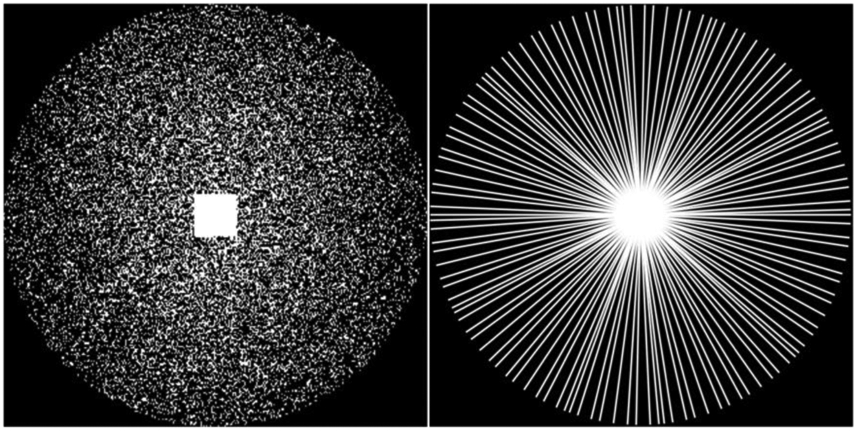
Sampling masks. Left: Cartesian trajectory. Right: Radial trajectory.
C.2. Quantitative evaluation metrics
We adopted Structural SIMilarity (SSIM) index, peak signal-to-noise ratio (PSNR), and normalized mean square error (NMSE) as evaluation metrics. Particularly, , , and , where is the reconstructed image, v is the image reconstructed from fully-sampled k-space data, is a squared Euclidean norm, max(v) is the largest value of v, n is the number of entries of v, , and μv are the average value of pixel intensities in and v respectively, and σv are their variances respectively, is the their covariance, and c1 = k1L and c2 = k2L are two variables to stabilize the division with L = max(v), k1 = 0.01, and k2 = 0.03 (Han et al., 2020). The evaluation metrics were computed and averaged based on the center slices of reconstructed images to exclude slices that lie outside the anatomy. Particularly, we chose the middle 200 slices of the test cases to evaluate the image reconstruction performance for Stanford dataset and all slices of the test cases for fastMRI dataset. The values of SSIM, PSNR, NMSE obtained by our method and those under comparison were also quantitatively compared using Wilcoxon signed-rank test.
C.3. Comparison with state-of-the-art methods
We compared our method with three different image-domain deep learning methods, including domain adaptation network (DA-Net) (Han et al., 2018), DeepcomplexMRI (Wang et al., 2020), spatial orthogonal attention generative adversarial network (SOGAN) (Zhou et al., 2020); two k-space deep learning methods, including RAKI (Akçakaya et al., 2019) and K-space deep learning (K-space-Net)(Han et al., 2020); and two hybrid deep learning methods in both the image-domain and k-space, including KIKI-Net (Eo et al., 2018) and Hybrid-Net (Souza et al., 2019). Particularly, DA-Net and K-space-Net were built upon the same U-net architecture as illustrated in Figure 1 (bottom). SOGAN, DeepcomplexMRI, KIKI-NET and Hybrid-Net were implemented with the number of model parameters similar to that of our method. RAKI was evaluated on uniformly undersampled data with a sampling rate close to 25%, following its original paper’s setting (Akçakaya et al., 2019). All the methods were evaluated on data generated with approximately the same acceleration rate of four.
Since all these methods under comparison learn the interpolation from individual image slices, for fair comparison we built two deep learning models using our method with the number of input slices c set to one and three, respectively. As illustrated in Figure 1, our network consisted of six encoding blocks, five decoding blocks, and one output block. The encoding and decoding blocks had convolutional layers with a receptive field of 3 × 3, ReLU layers, and BN layers, followed by attention layers. They were connected by pooling and unpooling layers to generate high-quality k-space data for image reconstruction. Number of kernels of the convolutional layers are specified in Figure 1 (bottom).
In addition, we evaluated the proposed ACNN-k-Space method as a plugin component in KIKI-Net (Eo et al., 2018) and Hybrid-Net (Souza et al., 2019), which are hybrid deep learning methods for MR image reconstruction in both the image domain (referred to as I-Nets) and k-space (referred to as K-Nets). Particularly, KIKI-Net comprises 2 K-Nets and 2 I-Nets in order of K-Net, I-Net, K-Net, and I-Net, each being CNNs with 5 layers, and the Hybrid-Net adds two more I-Nets to the KIKI-Net, one before and the other after the KIKI-Net. The K-Net in hybrid-Net has additional residual connection and data consistency layer compared with the K-Net in KIKI-Net.
To build a KIKI-Net and a Hybrid-Net with similar numbers of parameters as ACNN-k-Space, we implemented a KIKI-Net consisting of alternating five K-Nets and five I-Nets and a Hybrid-Net consisting of four K-Nets and six I-Nets, all in the same order as in their original versions. Each of the K-Nets and the I-Nets had five layers of CNNs with a receptive field of 3 × 3 and 256 kernels. Two versions of the KIKI-Net and Hybrid-Net were built with or without attention layers in their K-Nets for comparison. A public implementation of RAKI (https://qithub.com/geopi1/DeepMRI) was adopted in the present study. The total numbers of parameters of the other networks under comparison applied to Stanford and fastMRI datasets are summarized in Table 1.
Table 1.
Numbers of Parameters of different methods.
| Methods | Number of input slices | Stanford Dataset (Ncoil = 8) | fastMRI Dataset (Ncoil = 16) |
|---|---|---|---|
| DA-Net | 1 | 31.70M | 31.72M |
| K-space-Net | 1 | 31.70M | 31.72M |
| DeepcomplexMRI | 1 | 30.20M | 30.22M |
| SOGAN | 1 | 28.54M | 28.56M |
| ACNN-k-Space | 1 | 33.24M | 33.27M |
| ACNN-k-Space | 3 | 33.24M | 33.29M |
| KIKI-Net with attention | 1 | 37.80M | 37.81M |
| Hybrid-Net with attention | 1 | 37.80M | 37.81M |
C.4. Visualization of attention maps
In order to understand how the frequency-attention layers modulate CNN features, we directly visualized the frequency-attention maps at different layers of the network. In order to understand how the different channels of the multiple-channel input contribute to image reconstruction, we computed response value for each channel as ∥grad(C)∥1, where grad(C) is the gradient of a channel of the multiple-channel input once the network’s weights were obtained. Since the channel-attention maps at other layers of the network are learned from combinations of data of multiple coils from spatially adjacent slices, we could not map the response values of different channels to the input slices or coils.
C.5. Ablation studies
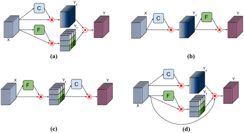
We carried out ablation studies to investigate the effectiveness of frequency-attention layers and channel-attention layers. These layers could learn attention weights in parallel or sequentially to module CNN features as illustrated in Figure 4. To integrate features modulated by parallel attention layers, as illustrated in Figure 4(a), we adopted an element-wise Max-out operator to fuse the modulated features. To modulate features sequentially, the channel-attention and frequency attention layers could be integrated differently as illustrated in in Figure 4(b) and Figure 4(c). Furthermore, the channel-attention and frequency-attention layers can also be applied in parallel to modulate their input simultaneously with an element-wise multiplication operator, as illustrated in Figure 4(d). In all these experiments, we set the number of input k-space slices to three. We finally evaluated how the image reconstruction performance changes with the number of input slices.
Figure 4.
Applications of attention layers. (a) The channel-attention and frequency-attention layers are applied in parallel and the modulated features are fused with an element-wise Max-out operator. (b) The channel-attention layer is applied before the frequency-attention layer. (c) The frequency-attention layer is applied before the channel-attention layer. (d) The channel-attention and frequency-attention layers are applied in parallel to modulate their input simultaneously with an element-wise multiplication operator.
These studies were carried out on Stanford dataset with Cartesian undersampling and fastMRI dataset with radial undersampling, respectively. Due to the high computational cost, we did not evaluate other possible combinations of input data and reconstruction settings.
C.6. Implementation and computing cost
We implemented all deep learning methods using PyTorch. Adam optimizer was used to train the network. Batch size was set to 16, number of training epochs set to 350, initial learning rate = 10−4 which gradually dropped to 10−5, and weight regularization parameter λ = 10−4.
All experiments were carried out on a Linux workstation equipped with 4 Titan XP GPUs with 12G memory. On a NVIDIA TITAN XP GPU, it took 50 milliseconds and 301 milliseconds for the deep learning models built by our method to reconstruct an image from undersampled Stanford k-space data (320×256×8) and fastMRI k-space data (640×320×16), respectively. It took ~50 hours to train a deep learning model on Stanford dataset and ~70 hours on fastMRI dataset.
Results
A. Image reconstruction performance
Image reconstruction performance comparisons are summarized in Tables 2 and 3 for Stanford and fastMRI datasets, respectively. These results demonstrate that our method consistently performed better than the deep learning methods under comparison with statistical significance (p<0.001), in particular with an input of multiple slices (three in the current implementation if not specified otherwise). Of note is that NMSE was reduced by 25% and 7% compared to image-domain and k-space based methods for the Stanford dataset, respectively, for Cartesian sampling. Further, NMSE was reduced by 10% and 7% compared to image-domain and k-space based methods for the fastMRI dataset, respectively, also for Cartesian sampling. The k-space deep learning methods also had better performance than their counterparts in the image domain (Han et al., 2018), consistent with previous findings (Han et al., 2020).
Table 2.
Comparison of the methods based on the Stanford dataset (mean±std).
| Methods | Number of input slices |
NMSE (× 10−3) ↓ | PSNR ↑ | SSIM (× 10−2) ↑ | |||
|---|---|---|---|---|---|---|---|
| Cartesian | Radial | Cartesian | Radial | Cartesian | Radial | ||
| DA-Net | 1 | 14.77±0.01 | 11.45±0.01 | 34.25±1.82 | 35.45±1.80 | 89.95±0.03 | 91.97±0.03 |
| DeepcomplexMRI | 1 | 13.20±0.01 | 11.33±0.01 | 34.82±1.52 | 35.52±1.44 | 90.95±0.02 | 92.57±0.02 |
| SOGAN | 1 | 12.93±0.01 | 11.32±0.01 | 34.75±1.36 | 35.48±1.29 | 90.96±0.03 | 92.47±0.03 |
| RAKI | 1 | 12.42±0.01 | 34.75±1.76 | 92.06±0.02 | |||
| k-space-Net | 1 | 11.98±0.01 | 11.26±0.01 | 35.27±1.89 | 35.56±1.82 | 92.05±0.02 | 92.65±0.03 |
| ACNN-k-Space | 1 | 11.55±0.01 | 11.22±0.01 | 35.45±1.81 | 35.57±1.78 | 92.15±0.03 | 92.65±0.03 |
| ACNN-k-Space | 3 | 11.11±0.01 | 10.90±0.01 | 35.55±1.86 | 35.63±1.82 | 92.25±0.03 | 92.73±0.03 |
Table 3.
Comparison of the methods based on the fastMRI brain dataset (mean±std).
| Methods | Number of input slices |
NMSE (× 10−3) ↓ | PSNR ↑ | SSIM (× 10−2) ↑ | |||
|---|---|---|---|---|---|---|---|
| Cartesian | Radial | Cartesian | Radial | Cartesian | Radial | ||
| DA-Net | 1 | 20.43±0.02 | 16.16±0.02 | 38.25±3.23 | 39.74±3.19 | 94.11±0.05 | 94.46±0.05 |
| DeepcomplexMRI | 1 | 20.58±0.02 | 16.15±0.02 | 38.26±2.67 | 39.75±2.88 | 94.03±0.04 | 94.48±0.05 |
| SOGAN | 1 | 19.98±0.02 | 15.99±0.02 | 38.40±2.34 | 38.83±2.67 | 94.28±0.04 | 94.54±0.05 |
| RAKI | 1 | 19.50±0.02 | 38.65±2.77 | 94.57±0.04 | |||
| k-space-Net | 1 | 19.67±0.02 | 15.71±0.02 | 38.60±2.97 | 39.85±3.26 | 94.58±0.05 | 94.61±0.05 |
| ACNN-k-Space | 1 | 18.80±0.02 | 15.29±0.02 | 38.95±3.20 | 40.11±3.27 | 94.62±0.05 | 94.86±0.05 |
| ACNN-k-Space | 3 | 18.30±0.02 | 14.93±0.02 | 39.16±3.03 | 40.39±3.30 | 95.02±0.05 | 95.21±0.05 |
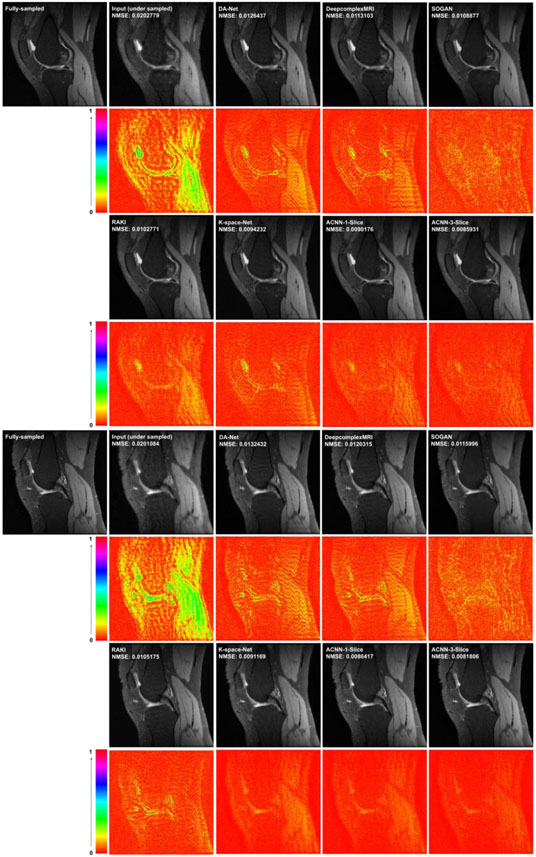
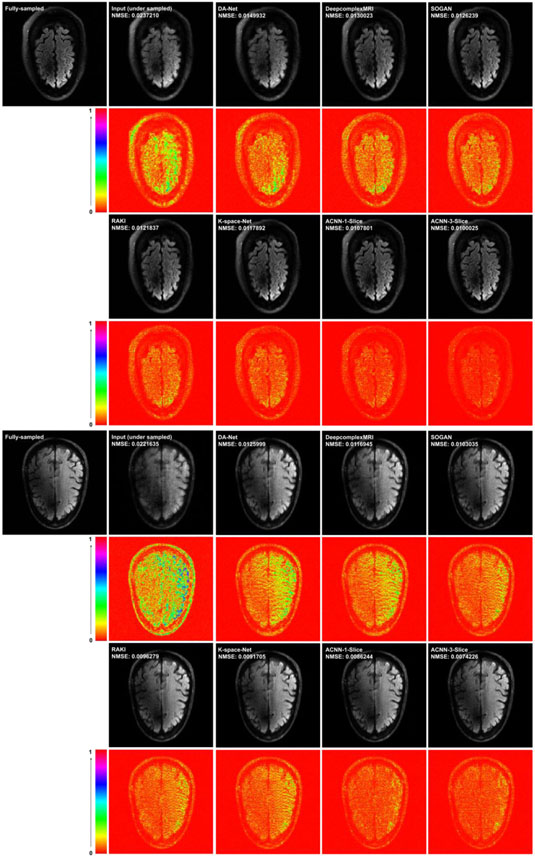
Figures 5 and 6 show representative results obtained for the different methods under comparison. Consistent with the quantitative results summarized in Tables 2 and 3, our method yielded visually better results than the alternative methods under comparison. In particular, the deep learning model in image domain yielded a slightly oversmoothed image. Further, the images reconstructed by our method had minimal difference with those reconstructed from the complete k-space data compared to the performance of the other deep learning methods either in the image domain or in k-space.
Figure 5.
Visualization of two representative cases of the Stanford knee dataset, including images reconstructed from the fully sampled data and from under-sampled data without CNN processing under Cartesian sampling (top) and radial sampling (bottom). The difference images were amplified 2 times. The number of coils of for the Stanford dataset was 8 and the acceleration factor was 4 with a sampling rate of 23.27%.
Figure 6.
Visualization of representative cases of the fastMRI brain dataset, including images reconstructed from the fully sampled data and from under-sampled data without CNN processing under Cartesian sampling (top) and radial sampling (bottom). The difference images were amplified 3 times for the fastMRI dataset. The number of coils for the fastMRI dataset was 16 and the acceleration factor was 4 with a sampling rate of 23.44%.
B. Visualization of attention maps
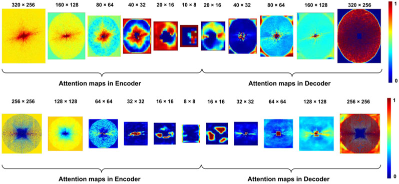
Figure 7 shows representative frequency-attention maps learned by our method with the number of input slices set to three for image reconstruction from undersampled k-space data using Cartesian sampling based on the Stanford dataset (top row) and radial sampling based on the fastMRI dataset (bottom row). Not surprisingly, the learned frequency-attention maps had varied weights at different spatial frequencies, indicating that k-space data at different frequencies contributed differently to the image reconstruction. It is worth noting that the last frequency-attention map largely complemented the downsampling sampling pattern to guarantee the network to generate a residual k-space interpolation map (lower attention to the sampled datapoints), which was added to the down-sampled k-space data through the residual connection (Figure 1) to reconstruct the image, leading to efficient and effective image reconstruction.
Figure 7.
Frequency-attention maps learned by the network for k-space data undersampled using Cartesian sampling (top) and radial sampling (bottom).
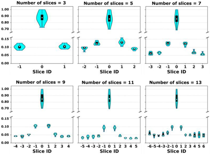
Figure 7 shows the response values of different channels grouped for individual slices for a representative test data of the Stanford dataset with the number of input slices set to 3, 5, 7, 9, 11, and 13, and using undersampled Cartesian k-space data. As expected, the channels (coils) of the center slice had the largest response values, and the response values decreased with distance from the center slice, indicating that the data of the center slice contributed most to image reconstruction while the influence decreases with distance from center.
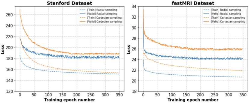
Figure 8 shows training loss functions for data undersampled with Cartesian sampling and the Radial sampling on Stanford and fastMRI datasets, respectively, indicating that ACNN-k-Space worked better on the training data with radial sampling than Cartesian sampling although they had the same acceleration factor.
Figure 8.
Visualization of response values of different channels of a testing case of the Stanford dataset. The response values were normalized by their max value. The response values are presented as violin plots to show the probability density of the data at different values, in addition to the median of the data and a box indicating the interquartile range.
C. Ablation studies
As summarized in Tables 4 and 5 on Stanford and fastMRI datasets, our ACNN-k-Space method with both frequency- and channel-attention layers yielded the best performance measures with statistical significance (p<0.001), while the k-space deep learning methods utilizing one attention layer still outperformed those without the self-attention layers.
Table 4.
Performance of the networks with different components on the Stanford dataset with Cartesian sampling.
| Methods | NMSE (× 10−3) ↓ | PSNR ↑ | SSIM (× 10−2) ↑ | |||
|---|---|---|---|---|---|---|
| Mean±std | p-value | Mean±std | p-value | Mean±std | p-value | |
| Without self-attention | 11.95±0.01 | 7.4e-63 | 35.19±1.81 | 1.1e-59 | 92.04±0.02 | 2.0e-40 |
| Channel-attention alone | 11.52±0.01 | 9.7e-50 | 35.39±1.83 | 8.4e-48 | 92.15±0.03 | 8.1e-38 |
| Frequency-attention alone | 11.43±0.01 | 7.8e-37 | 35.43±1.87 | 5.3e-3 | 92.17±0.03 | 1.1e-17 |
| ACNN-k-Space | 11.11±0.01 | - | 35.55±1.86 | - | 92.25±0.03 | - |
Table 5.
Performance of networks with different components on the fastMRI dataset with radial sampling.
| Methods | NMSE (× 10−3) ↓ | PSNR ↑ | SSIM (↓ 10−2) ↑ | |||
|---|---|---|---|---|---|---|
| mean±std | p-value | mean±std | p-value | mean±std | p-value | |
| Without self-attention | 15.47±0.02 | 1.90e-6 | 40.00±3.15 | 3.14e-9 | 94.83±0.05 | 2.67e-11 |
| Channel-attention alone | 15.25±0.03 | 5.61e-5 | 40.13±3.05 | 9.14e-7 | 94.94±0.05 | 4.19e-10 |
| Frequency-attention alone | 15.11±0.02 | 5.44e-6 | 40.23±3.02 | 3.37e-6 | 95.03±0.06 | 3.29e-12 |
| ACNN-k-Space | 14.93±0.02 | - | 40.39±3.25 | - | 95.21±0.05 | - |
As summarized in Tables 6 and 7 on Stanford and fastMRI datasets, the k-space deep learning method with F-C (frequency-attention layer followed by channel-attention layer) attention block and C-F (channel-attention layer followed by frequency-attention layer) attention block performed better than CF-X (channel-attention and frequency-attention layers applied in parallel to modulate their input simultaneously), while the parallel frequency-attention and channel-attention layers yielded the best performance.
Table 6.
Performance of different attention blocks on the Stanford dataset under Cartesian sampling (the architectures are ranked based on NMSE).
Table 7.
Performance of different attention blocks on the fastMRI dataset under radial sampling (the architectures are ranked based on NMSE).
As summarized in Tables 8 and 9, image reconstruction performance increased with the number of input slices, although some of the improvements were small. We expect that the method will reach its peak performance with a moderately large number of input slices. However, the computational cost will also increase with the number of input slices, while the incremental gain becomes increasingly smaller. Further, some datasets will be limited by the number of available slices. It is worth noting that for the fastMRI brain dataset, inputs with more than 3 slices largely overlap with each other in that the inputs were often padded with the bottom-most or the top-most slice.
Table 8.
Performance of our method with different numbers of the input slices based on the Stanford dataset.
| Number of input slices |
NMSE (× 10−3) ↓ | PSNR ↑ | SSIM (× 10−2) ↑ | Train times | Test time (each case) |
|||
|---|---|---|---|---|---|---|---|---|
| Mean±std | p-value | Mean±std | p-value | Mean±std | p-value | |||
| 11.55±0.01 | - | 35.45±1.81 | - | 92.15±0.03 | - | ~44 hours | ~49 ms | |
| 11.11±0.01 | 7.4e-63 | 35.55±1.86 | 2.1e-53 | 92.25±0.03 | 6.3e-30 | ~50 hours | ~50 ms | |
| 10.94±0.00 | 1.3e-64 | 35.57±1.84 | 5.1e-61 | 92.30±0.03 | 2.2e-42 | ~57 hours | ~58 ms | |
| 10.76±0.00 | 2.0e-66 | 35.61±1.84 | 1.1e-61 | 92.35±0.03 | 8.8e-45 | ~65 hours | ~62 ms | |
| 10.65±0.00 | 1.1e-65 | 35.64±1.84 | 1.2e-61 | 92.40±0.03 | 2.4e-45 | ~74 hours | ~65 ms | |
| 11 | 10.64±0.00 | 2.9e-66 | 35.64±1.84 | 1.1e-61 | 92.45±0.03 | 9.7e-46 | ~84 hours | ~70 ms |
Table 9.
Performance of our method with different numbers of the input slices based on the fastMRI dataset.
| Number of input slices |
NMSE (× 10−3) ↓ | PSNR ↑ | SSIM (× 10−2) ↑ | Train time | Test time (each case) |
|||
|---|---|---|---|---|---|---|---|---|
| Mean±std | p-value | Mean±std | p-value | Mean±std | p-value | |||
| 15.29±0.02 | - | 40.11±3.27 | - | 94.86±0.05 | - | ~62 hours | ~58 ms | |
| 14.93±0.02 | 2.6e-2 | 40.39±3.30 | 5.1e-2 | 95.21±0.05 | 5.6e-3 | ~70 hours | ~60 ms | |
| 14.72±0.02 | 4.6e-6 | 40.49±2.88 | 3.3e-7 | 95.42±0.05 | 1.9e-8 | ~79 hours | ~64 ms | |
| 14.60±0.02 | 1.5e-9 | 40.55±2.92 | 6.0e-9 | 95.48±0.05 | 8.3e-12 | ~89 hours | ~69 ms | |
| 14.55±0.02 | 8.3e-7 | 40.58±2.90 | 9.3e-8 | 95.50±0.05 | 6.3e-10 | ~101 hours | ~73 ms | |
| 11 | 14.51±0.02 | 3.7e-9 | 40.62±3.02 | 7.8e-8 | 96.51±0.05 | 5.3e-11 | ~113hours | ~78 ms |
D. ACNN-k-Space in hybrid deep learning methods for MR image reconstruction
As summarized in Tables 10 and 11, KIKI-Net and Hybrid-Net with attention layers in their K-Nets achieved significantly better image reconstruction performance with statistical significance (p<0.001) than their original version (Eo et al., 2018; Souza et al., 2019) on both Stanford and fastMRI brain datasets. Particularly, NMSE was reduced by 1% to 4% by using the attention layers in KIKI-Net and Hybrid-Net. Reconstruction results of representative images obtained by KIKI-Net and Hybrid-Net with and without attention layers are shown in Figure 9.
Table 10.
Performance of hybrid deep learning methods with and without the attention layers in their k-space deep learning components on the Stanford dataset.
| Methods | NMSE (× 103) ↓ | PSNR ↑ | SSIM (× 10∈2) ↑ | |||||||||
|---|---|---|---|---|---|---|---|---|---|---|---|---|
| Cartesian | Radial | Cartesian | Radial | Cartesian | Radial | |||||||
| mean±std | p-value | mean±std | p-value | mean±std | p-value | mean±std | p-value | mean±std | p-value | mean±std | p-value | |
| KIKI-Net | 10.96±0.01 | 2.1e-23 | 10.44±0.01 | 9.6e-22 | 35.71±1.75 | 5.5e-32 | 35.91±1.72 | 2.5e-39 | 91.98±0.02 | 9.7e-24 | 92.78±0.02 | 4.1e-24 |
| w/attention | 10.84±0.01 | - | 10.08±0.01 | - | 35.76±1.74 | - | 36.07±1.76 | - | 92.00±0.02 | - | 92.80±0.02 | - |
| Hybrid-Net | 10.77±0.01 | 9.5e-22 | 10.39±0.01 | 7.4e-17 | 35.79±1.63 | 4.3e-32 | 35.95±1.67 | 1.7e-34 | 91.98±0.02 | 3.5e-21 | 92.81±0.02 | 1.6e-19 |
| w/attention | 10.40±0.01 | - | 10.01±0.01 | - | 35.95±1.59 | - | 36.11±1.70 | - | 92.13±0.02 | - | 92.84±0.02 | - |
Table 11.
Performance of hybrid deep learning methods with and without the attention layers in their k-space deep learning components on the fastMRI dataset.
| Methods | NMSE (× 10−3) ↓ | PSNR ↑ | SSIM (× 10−2) ↑ | |||||||||
|---|---|---|---|---|---|---|---|---|---|---|---|---|
| Cartesian | Radial | Cartesian | Radial | Cartesian | Radial | |||||||
| mean±std | p-value | mean±std | p-value | mean±std | p-value | mean±std | p-value | mean±std | p-value | mean±std | p-value | |
| KIKI-Net | 18.02±0.02 | 7.5e-25 | 14.70± 0.02 | 3.8e-24 | 39.27±3.03 | 7.2e-36 | 40.51±3.30 | 6.8e-32 | 95.12±0.05 | 1.6e-22 | 95.29±0.05 | 4.4e-19 |
| w/attention | 17.84±0.01 | - | 14.38±0.01 | - | 39.36±2.53 | - | 40.65±3.06 | - | 95.18±0.05 | - | 95.35±0.04 | - |
| Hybrid-Net | 17.89±0.01 | 6.3e-22 | 14.66±0.01 | 1.8e-19 | 39.32±2.63 | 4.9e-27 | 40.59±3.04 | 9.2e-27 | 95.15±0.05 | 1.4e-22 | 95.32±0.05 | 2.8e-16 |
| w/attention | 17.64±0.01 | 14.38±0.01 | - | 39.40±2.74 | - | 40.69±2.86 | - | 95.20±0.04 | - | 95.39±0.04 | - | |
Figure 9.
Visualization of training and validation loss functions for data undersampled with Cartesian and radial sampling. The loss functional values were normalized by the image size (width × length).
Discussion
We have developed a novel deep learning method for image reconstruction from undersampled k-space data. Our method is built upon a residual Encoder-Decoder network of CNNs to learn interpolation in k-space. Also, rather than learning the interpolation independently for each slice, we integrate complementary information of spatially adjacent slices as multi-channel input to the residual network to improve image reconstruction. We adopt self-attention layers to effectively integrate complementary information of multiple slices and recognize distinctive contributions of k-space data at different spatial frequencies. Ablation studies and comparison with existing methods have demonstrated that our method could effectively reconstruct images from undersampled k-space data and achieved significantly better image reconstruction performance than state-of-the-art alternative techniques.
Our method adaptively learns k-space data interpolation using self-attention layers consisting of frequency-attention and channel-attention layers. As illustrated in Figure 6, the frequency-attention maps had distinctive values at different spatial frequencies of the k-space data, indicating that the frequency-attention layers could modulate features learned by weight-sharing CNNs so that the deep learning models could model k-space data at low and high frequencies differently. As illustrated in Figure 7, the channel-attention layers facilitate effective integration of information from spatially adjacent image slices. It has been demonstrated that channel-attention is a powerful technique to improve image reconstruction by integrating channel-wise features adaptively rather than equally (Huang et al., 2019; Lee et al., 2020). Our results provide additional evidence that the channel-attention layer applied to input image slices could also improve the image reconstruction performance. Quantitative evaluation results summarized in Tables 2 and 3 have further demonstrated that the attention layers could effectively improve the image reconstruction performance compared with deep learning models without the attention layers with only a 5% increase in the number of model parameters.
The ablation experimental results have further demonstrated that the self-attention layers in conjunction with the residual Encoder-Decoder network architecture can improve k-space data interpolation. Particularly, results summarized in Tables 4 and 5 demonstrate that the self-attention layers, especially when both the channel-attention and the frequency-attention layers were used jointly, achieved significantly better image reconstruction performance than deep learning models without the attention layers or with only one type of attention layers. The results summarized Table 6 and Table 7 have demonstrated that the parallel architecture has achieved better performance than the alterative architectures. Finally, the results summarized in Table 8 and Table 9 have further demonstrated that integration of information from spatially adjacent image slices of the image slice under consideration can improve the image reconstruction performance.
As demonstrated by the results summarized in Tables 10 and 11 and visualized in Figure 9, the attention layers improved the image reconstruction performance of KIKI-Net and Hybrid-Net (Eo et al., 2018; Souza et al., 2019) compared with their original version with statistical significance though the differences were relatively subtle, indicating that the attention layers might be useful as a plugin component in other k-space deep learning methods to improve the image reconstruction performance. Given that the image reconstruction performance can be improved when more image slices are used as input (Tables 2, 3, 8, and 9), we expect that KIKI-Net and Hybrid-Net could be further improved with multiple image slices as their input in conjunction with the attention layers.
Our method achieved slightly better performance for the undersampled data generated with radial and spiral undersampling trajectories than Cartesian and 1-D undersampling trajectories, as demonstrated by the results shown in Figure 8 and Table S1. We postulate that this is caused by the fact that radial and spiral undersampling trajectories generally contain more data points at low spatial frequency regions than Cartesian and 1-D undersampling trajectories at the same undersampling rate. However, this issue merits a more rigorous investigation, which will be a focus of future studies. Interestingly, our method implemented with L1 loss and L2 loss yielded similar performance on the Stanford dataset, as summarized in Table S2. A recent study has demonstrated that perceptual loss function performed significantly better than L1 or L2 loss functions as determined by radiologists’ scores (Ghodrati et al., 2019). We will evaluate if adopting the perceptual loss function in our network will improve the image reconstruction performance.
Our network is built upon the standard residual Encoder-Decoder network architecture, which has also achieved promising performance in image segmentation (Li et al., 2021) and could be improved by adopting other network architectures, network blocks, and advanced learning strategies, such as Dense block (Huang et al., 2017), or instance normalization (Ulyanov et al., 2016), in conjunction with advanced loss function (Ledig et al., 2017). It is noteworthy that a variety of deep-learning MR reconstruction methods have been developed recently, such as cascaded networks (Huang et al., 2019; Qin et al., 2018), variational network (Sriram et al., 2020), RARE (Liu et al., 2019), and DeepcomplexMRI network (Wang et al., 2020). Our method could also be adopted in these methods as a basic deep learning component to improve their image reconstruction performance.
In conclusion, we have developed adaptive CNNs for k-space data interpolation which has achieved favorable performance compared with state-of-the-art deep learning methods.
Supplementary Material
Figure 10.
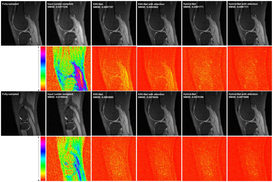
Visualization of representative cases of Stanford dataset, including images reconstructed from KIKI-Net and Hybrid-Net with and without attention layers under Cartesian sampling (top) and radial sampling (bottom). The difference images were amplified by 4. The number of coils was 8 and the acceleration factor was 4.
highlights.
Adaptive CNNs are used for accelerating magnetic resonance imaging
Self-attention facilitates adaptive learning of k-space data
Complementary information of spatially adjacent slices is integrated
Common weight-sharing CNNs are ineffective for k-space data interpolation
The method achieves significantly improved image reconstruction performance
Acknowledgement
Research reported in this study was partially supported by the National Institutes of Health under award number [R01EB022573, R01MH120811, and U24CA231858]. The content is solely the responsibility of the authors and does not necessarily represent the official views of the National Institutes of Health.
Footnotes
Declaration of interests
The authors declare that they have no known competing financial interests or personal relationships that could have appeared to influence the work reported in this paper.
Publisher's Disclaimer: This is a PDF file of an unedited manuscript that has been accepted for publication. As a service to our customers we are providing this early version of the manuscript. The manuscript will undergo copyediting, typesetting, and review of the resulting proof before it is published in its final form. Please note that during the production process errors may be discovered which could affect the content, and all legal disclaimers that apply to the journal pertain.
References
- Abdullah S, Arif O, Arif MB, Mahmood T, 2019. MRI Reconstruction from sparse K-space data using low dimensional manifold model. IEEE Access 7, 88072–88081. [Google Scholar]
- Agarap AF, 2018. Deep learning using rectified linear units (relu). arXiv preprint arXiv:1803.08375. [Google Scholar]
- Aggarwal HK, Mani MP, Jacob M, 2019. MoDL: Model-Based Deep Learning Architecture for Inverse Problems. IEEE Transactions on Medical Imaging 38, 394–405. [DOI] [PMC free article] [PubMed] [Google Scholar]
- Akçakaya M, Moeller S, Weingärtner S, Uğurbil K, 2019. Scan-specific robust artificial-neural-networks for k-space interpolation (RAKI) reconstruction: Database-free deep learning for fast imaging. Magnetic Resonance in Medicine 81, 439–453. [DOI] [PMC free article] [PubMed] [Google Scholar]
- Beatty PJ, Nishimura DG, Pauly JM, 2005. Rapid gridding reconstruction with a minimal oversampling ratio. IEEE transactions on medical imaging 24, 799–808. [DOI] [PubMed] [Google Scholar]
- Cheng JY, Mardani M, Alley MT, Pauly JM, Vasanawala S, 2018. DeepSPIRiT: generalized parallel imaging using deep convolutional neural networks, Proc. 26th Annual Meeting of the ISMRM, Paris, France. [Google Scholar]
- Duda K, 2011. DFT interpolation algorithm for Kaiser–Bessel and Dolph–Chebyshev windows. IEEE Transactions on Instrumentation and Measurement 60, 784–790. [Google Scholar]
- Eo T, Jun Y, Kim T, Jang J, Lee HJ, Hwang D, 2018. KIKI - net: cross - domain convolutional neural networks for reconstructing undersampled magnetic resonance images. Magnetic resonance in medicine 80, 2188–2201. [DOI] [PubMed] [Google Scholar]
- Fessler JA, Sutton BP, 2003. Nonuniform fast Fourier transforms using min-max interpolation. IEEE transactions on signal processing 51, 560–574. [Google Scholar]
- Ghodrati V, Shao J, Bydder M, Zhou Z, Yin W, Nguyen K-L, Yang Y, Hu P, 2019. MR image reconstruction using deep learning: evaluation of network structure and loss functions. Quantitative Imaging in Medicine and Surgery 9, 1516–1527. [DOI] [PMC free article] [PubMed] [Google Scholar]
- Hammernik K, Klatzer T, Kobler E, Recht MP, Sodickson DK, Pock T, Knoll F, 2018. Learning a variational network for reconstruction of accelerated MRI data. Magnetic Resonance in Medicine 79, 3055–3071. [DOI] [PMC free article] [PubMed] [Google Scholar]
- Han Y, Sunwoo L, Ye JC, 2020. k-Space Deep Learning for Accelerated MRI. IEEE Trans Med Imaging 39, 377–386. [DOI] [PubMed] [Google Scholar]
- Han Y, Yoo J, Kim HH, Shin HJ, Sung K, Ye JC, 2018. Deep learning with domain adaptation for accelerated projection - reconstruction MR. Magnetic resonance in medicine 80, 1189–1205. [DOI] [PubMed] [Google Scholar]
- Hu J, Shen L, Sun G, 2018. Squeeze-and-Excitation Networks, 2018 IEEE/CVF Conference on Computer Vision and Pattern Recognition, pp. 7132–7141. [Google Scholar]
- Huang G, Liu Z, Maaten L.v.d., Weinberger KQ, 2017. Densely connected convolutional networks, 2017 IEEE Conference on Computer Vision and Pattern Recognition, pp. 4700–4708. [Google Scholar]
- Huang Q, Yang D, Wu P, Qu H, Yi J, Metaxas D, 2019. MRI reconstruction via cascaded channel-wise attention network, 2019 IEEE 16th International Symposium on Biomedical Imaging (ISBI 2019). IEEE, pp. 1622–1626. [Google Scholar]
- Ioffe S, Szegedy C, 2015. Batch normalization: Accelerating deep network training by reducing internal covariate shift. arXiv preprint arXiv:1502.03167. [Google Scholar]
- Jin KH, McCann MT, Froustey E, Unser M, 2017. Deep Convolutional Neural Network for Inverse Problems in Imaging. IEEE Transactions on Image Processing 26, 4509–4522. [DOI] [PubMed] [Google Scholar]
- Kim TH, Garg P, Haldar JP, 2019. LORAKI: Autocalibrated recurrent neural networks for autoregressive MRI reconstruction in k-space. arXiv preprint arXiv:1904.09390. [Google Scholar]
- Knoll F, Hammernik K, Zhang C, Moeller S, Pock T, Sodickson DK, Akcakaya M, 2020. Deep-Learning Methods for Parallel Magnetic Resonance Imaging Reconstruction: A Survey of the Current Approaches, Trends, and Issues. IEEE Signal Processing Magazine 37, 128–140. [DOI] [PMC free article] [PubMed] [Google Scholar]
- Ledig C, Theis L, Huszár F, Caballero J, Cunningham A, Acosta A, Aitken A, Tejani A, Totz J, Wang Z, 2017. Photo-realistic single image super-resolution using a generative adversarial network, Proceedings of the IEEE conference on computer vision and pattern recognition, pp. 4681–4690. [Google Scholar]
- Lee D, Yoo J, Tak S, Ye JC, 2018. Deep Residual Learning for Accelerated MRI Using Magnitude and Phase Networks. IEEE Transactions on Biomedical Engineering 65, 1985–1995. [DOI] [PubMed] [Google Scholar]
- Lee J, Kim H, Chung H, Ye JC, 2020. Deep Learning Fast MRI Using Channel Attention in Magnitude Domain, 2020 IEEE 17th International Symposium on Biomedical Imaging (ISBI), pp. 917–920. [Google Scholar]
- Li Y, Li H, Fan Y, 2021. ACEnet: Anatomical context-encoding network for neuroanatomy segmentation. Medical Image Analysis 70, 101991. [DOI] [PMC free article] [PubMed] [Google Scholar]
- Liang D, Cheng J, Ke Z, Ying L, 2020. Deep Magnetic Resonance Image Reconstruction: Inverse Problems Meet Neural Networks. IEEE Signal Processing Magazine 37, 141–151. [DOI] [PMC free article] [PubMed] [Google Scholar]
- Liu J, Sun Y, Eldeniz C, Gan W, An H, Kamilov US, 2019. RARE: Image Reconstruction using Deep Priors Learned without Ground Truth. arXiv:1912.05854. [Google Scholar]
- Qin C, Schlemper J, Caballero J, Price AN, Hajnal JV, Rueckert D, 2018. Convolutional recurrent neural networks for dynamic MR image reconstruction. IEEE transactions on medical imaging 38, 280–290. [DOI] [PubMed] [Google Scholar]
- Quan TM, Nguyen-Duc T, Jeong WK, 2018. Compressed Sensing MRI Reconstruction Using a Generative Adversarial Network With a Cyclic Loss. IEEE Transactions on Medical Imaging 37, 1488–1497. [DOI] [PubMed] [Google Scholar]
- Ronneberger O, Fischer P, Brox T, 2015. U-net: Convolutional networks for biomedical image segmentation, International Conference on Medical image computing and computer-assisted intervention. Springer, pp. 234–241. [Google Scholar]
- Roy AG, Navab N, Wachinger C, 2018. Recalibrating fully convolutional networks with spatial and channel “squeeze and excitation” blocks. IEEE transactions on medical imaging 38, 540–549. [DOI] [PubMed] [Google Scholar]
- Schlemper J, Caballero J, Hajnal JV, Price AN, Rueckert D, 2018. A Deep Cascade of Convolutional Neural Networks for Dynamic MR Image Reconstruction. IEEE Trans Med Imaging 37, 491–503. [DOI] [PubMed] [Google Scholar]
- Souza R, Lebel RM, Frayne R, 2019. A hybrid, dual domain, cascade of convolutional neural networks for magnetic resonance image reconstruction, International Conference on Medical Imaging with Deep Learning, pp. 437–446. [Google Scholar]
- Sriram A, Zbontar J, Murrell T, Defazio A, Zitnick CL, Yakubova N, Knoll F, Johnson P, 2020. End-to-End Variational Networks for Accelerated MRI Reconstruction. arXiv preprint arXiv:2004.06688. [Google Scholar]
- Ulyanov D, Vedaldi A, Lempitsky V, 2016. Instance normalization: The missing ingredient for fast stylization. arXiv preprint arXiv:1607.08022. [Google Scholar]
- Wang S, Cheng H, Ying L, Xiao T, Ke Z, Zheng H, Liang D, 2020. DeepcomplexMRI: Exploiting deep residual network for fast parallel MR imaging with complex convolution. Magnetic Resonance Imaging 68, 136–147. [DOI] [PubMed] [Google Scholar]
- Wang S, Su Z, Ying L, Peng X, Zhu S, Liang F, Feng D, Liang D, 2016. Accelerating magnetic resonance imaging via deep learning, 2016 IEEE 13th International Symposium on Biomedical Imaging (ISBI), pp. 514–517. [DOI] [PMC free article] [PubMed] [Google Scholar]
- Zbontar J, Knoll F, Sriram A, Muckley MJ, Bruno M, Defazio A, Parente M, Geras KJ, Katsnelson J, Chandarana H, 2018. fastMRI: An open dataset and benchmarks for accelerated MRI. arXiv preprint arXiv:1811.08839. [Google Scholar]
- Zhou W, Du H, Mei W, Fang L, 2020. Spatial orthogonal attention generative adversarial network for MRI reconstruction. Medical Physics. [DOI] [PubMed] [Google Scholar]
- Zhu B, Liu JZ, Cauley SF, Rosen BR, Rosen MS, 2018. Image reconstruction by domain-transform manifold learning. Nature 555, 487–492. [DOI] [PubMed] [Google Scholar]
Associated Data
This section collects any data citations, data availability statements, or supplementary materials included in this article.


