A note on modeling placement values in the analysis of receiver operating characteristic curves

Abstract

Recent advances in receiver operating characteristic (ROC) curve analyses advocate modeling of placement value (PV), a quantity that measures the position of diseased test scores relative to the healthy population. Compared to traditional approaches, this PV-based alternative works directly with ROC curves and is attractive when assessing covariate effects on, or incorporating a priori constraints of, ROC curves. Several distributions can be used to model the PV, yet little guidelines exist in the literature on which to use. Through extensive simulation studies, we investigate several parametric models for PV when data are generated from a variety of mechanisms. We discuss the pros and cons of each of these models and illustrate their applications with data from a study of prenatal ultrasound examinations and large-for-gestational age birth.

1. Introduction

The receiver operating characteristic (ROC) curve is a widely used statistical methodology to evaluate the capacity of a test in distinguishing subjects with a condition (e.g., diseased) from those without (e.g., healthy). As a plot of true versus false positive rates for all possible threshold values, the ROC curve provides a useful tool to visualize the tradeoff between sensitivity and specificity of the test. The area under the ROC curve (AUC) is often used as a summary measure of the discriminatory capacity of the test. Zhou et al. (2002) and Pepe (2003) provide detailed developments of ROC analysis and contain comprehensive review of related literature.

Early approaches to ROC analysis focus primarily on distributions of the test scores. More recently, researchers have proposed modeling of placement values (Alonzo and Pepe, 2002; Cai, 2004; Dodd and Pepe, 2003; Pepe and Cai, 2004). Briefly speaking, a placement value (PV) of a diseased test score is the proportion of healthy test scores with values larger than it, and quantifies the separation between diseased and healthy populations (Hanley and HajianTilaki, 1997). This new conceptual framework for ROC analysis allows direct modeling of covariate effects on the ROC curves and accommodates a priori constraints if available, among others.

Few guidelines exist in the literature on models for the placement value, a quantity whose theoretical properties are not well-known. Stanley and Tubbs (2018) consider normal and Beta distributions for PVs but concern mostly about the consequence of parametric versus nonparametric specifications of the baseline ROC curve in the context of a regression framework (Rodriguez-Alvarez et al., 2011). In this note, we aim to fill this gap by conducting an in-depth simulation study to compare the performance of different models for the placement values. We consider a spectrum of scenarios by varying data generating mechanisms, sample sizes, and AUC values. The competing models in consideration are evaluated based on how well they estimate the ROC curves and AUCs.

The rest of the paper is organized as follows. In Section 2 we introduce ROC analysis based on placement values and detail the competing models for PV. In Section 3 we describe simulation set up, define measures for evaluating performance, and interpret simulation results. Section 4 presents applications of the models to data from a study of prenatal ultrasound examination and large-for-gestational age birth. We provide concluding remarks in Section 5.

2. Methods

2.1. ROC curves and placement values

Let X and Y represent continuous test scores from a healthy and a diseased population, respectively, with corresponding cumulative distribution functions (CDF) F₀ and F₁. Traditional approaches to ROC analysis proceed with specifying F₀ and F₁ and expressing the ROC curve as $ROC(t)=1-F_0\left(F_1^{-1}(1-t)\right)$ for t ∈ (0, 1). One such traditional model is the Bi-Normal model (Metz, 1986) which stipulates that X and Y are both normally distributed with varying means and variances. Alternatively, one can work with F₀ and the distribution F_Z of the placement value of a diseased test score y in F₀, Z = P(X > y) = 1 − F₀(y). It is easy to show that ROC(t) = F_Z(t). Furthermore, since the expected value of a random variable is the area under its survival function, AUC = 1 − E(Z). Compared to traditional approaches, the PV-based alternative allows direct modeling of the ROC curve and AUC, which can be quite useful when it is of interest to assess covariate effects on, or to accommodate a priori constraints of, ROC curve and AUC. The PV-based approach to ROC analysis involves estimating F₀ and obtaining Z in a first stage and modeling Z in a second stage. To obtain Z, one can estimate S₀ = 1− F₀ using a parametric regression model. Alternatively a flexible semiparametric location model (Heagerty and Pepe, 1999; Pepe, 1997) or linear transformation models can be used. Since the goal of this paper is to evaluated performances of several competing models for Z, we focus on the second stage modeling process and assume that a realization z = (z_i …, z_n) from F_Z is already available.

2.2. Logit- and Probit-Normal models

Since Z has support on the unit interval (0, 1), we can apply some appropriate transformation, say τ, to map it onto the real line and then model the transformed variable τ(Z) with a normal model:

$$\tau (Z)~N\left(\mu ,{\sigma }^2\right),$$

where N(μ, σ²) denotes a normal distribution with mean μ and variance σ². Then an estimator of ROC curve can be obtained as

$$ROC(t)=\Phi \left(\frac{\tau (t)-\mu }{\sigma }\right),t\in (0,1),$$

where Φ is the standard normal CDF. Since AUC = 1− E(Z), an estimator of the AUC is

$$AUC=1-{\tau }^{-1}(\mu ),$$ (2.1)

where τ⁻¹ is the inverse function of τ. We consider two choices of τ: logit where $\tau (s)=\text{log}\left(\frac{s}{1-s}\right)$ and probit where τ(s) = Φ⁻¹(s) and Φ⁻¹ is the inverse function of Φ. Note that the Probit-Normal model is equivalent to the parametric distribution-free model in Pepe and Cai (2004) without covariate, and is also equivalent to the Bi-Normal model.

2.3. The Log-Normal model

Another choice to model Z is the lognormal model

$$Z~LN\left(\theta ,{\lambda }^2\right),$$

where LN(θ, λ²) denotes a lognormal distribution with mean $e^{\theta +{\lambda }^2/2}$. Under this model, the ROC curve can be expressed as

$$\mathit{\text{ROC}}(t)=\Psi (t,\theta ,\lambda ),t\in (0,1),$$

where Ψ(t, θ, λ) is the CDF of LN(θ, λ) evaluated at t. The AUC is then

$$AUC=1-e^{\theta +{\lambda }^2/2}.$$ (2.2)

2.4. The Beta model

The Beta distribution is a reasonable choice given the unit interval support of Z,

$$Z~B(p,q),$$

where B(p, q) denotes a Beta distribution with mean p/(p + q). The ROC curve can be derived as

$$ROC(t)=\Lambda (t,p,q),t\in (0,1),$$

where Λ(t, p, q) is the CDF of B(p, q) evaluated at t, and the AUC estimator is

$$AUC=\frac{q}{p+q}.$$ (2.3)

2.5. Estimations

In all models above, we obtain maximum likelihood estimators (MLEs) of the model parameters (μ, σ, θ, λ, p, q). ROC curves and AUCs are then estimated by plugging in these MLEs. When necessary, delta method is used to obtain standard error estimates of AUCs. Since E(Z) = τ⁻¹(μ) is not generally true (except when τ is a linear transformation), we also consider a sampling-based alternative to the analytic-based AUC estimator in equation (2.1). Taking advantage of the relationship between AUC and Z, we can generate a sample $z_1^{*},\dots ,z_m^{*}$ from the predictive distributions of Z after obtaining estimates of model parameters. Then the sampling-based AUC estimator can be obtained as

$$\widehat{AU{C}^{*}}=1-\frac{1}{m}\sum _i^m{z}_i^{*}.$$ (2.4)

For completeness, we also obtained similar sampling-based estimators for the Log-Normal and Beta models.

3. Simulations

3.1. Data generating mechanisms

Our simulations proceed by first specifying the true distributions of the healthy and diseased score distributions F₀ and F₁. Although one can generate $x_1,\dots ,x_{n_0}$ from F₀, y₁, …, y_n from F₁, and calculate $z_i=\frac{1}{n_0}{\sum }_{j=1}^{n_0}I\left(x_j>y_i\right)$, i = 1, …, n, we instead generate the y’s only and let z_i = 1− F₀(y_i), i = 1, …, n. We consider three data generating mechanisms as follows.

In the Bi-Normal (BNM) mechanism, X and Y are normally distributed as $N\left({\mu }_1,{\sigma }_1^2\right)$ and $N\left({\mu }_1,{\sigma }_1^2\right)$. The true ROC curve and AUC are given by

$$ROC(t)=\Phi \left(a+b{\Phi }^{-1}(t)\right),AUC=\Phi \left(\frac{a}{\sqrt{1+b^2}}\right),$$

where $a=\frac{{\mu }_1-{\mu }_0}{{\sigma }_1}$ and $b=\frac{{\sigma }_0}{{\sigma }_1}$.

Similar to the Bi-Normal model, the Bi-Gamma (BGM, Bandos et al. (2017); Dorfman et al. (1997)) mechanism assumes that both X and Y follow gamma distributions with scales θ₀ and θ₁ and a common shape κ: X ~ GAM(θ₀, κ) and Y ~ GAM(θ₁, κ), where GAM(ν₁, ν₂) stands for a gamma distribution with scale ν₁ and shape ν₂. The corresponding true AUC is given by

$$AUC=1-H_{2\kappa ,2\kappa }\left(\frac{{\theta }_0}{{\theta }_1}\right),$$

where Hυ_1, υ₂ is CDF of the F distribution with degrees of freedom υ₁ and υ ₂. In the special case of θ₀ = 1 the ROC curve has a closed form expression

$$ROC(t)=1-G_{\kappa }\left(\frac{1}{{\theta }_1}{G}_{\kappa }^{-1}(1-t)\right),$$

where G_ν(t) is the CDF of a gamma distribution with scale 1 and shape ν evaluated at t and $G_{\kappa }^{-1}$ is its inverse function.

A Bi-Mixture-Normal model (BMN, Dass and Kim (2011)) is also considered where X ~ N(0, 1) and Y ~ MN(μ, σ², π), where MN(μ, σ², π) is a K-component mixture of normals distribution with μ = (μ₁, …, μ_K), ${\sigma }^2=\left({\sigma }_1^2,\dots ,{\sigma }_K^2\right)$ and π = (π₁, …, π_K). Here the weights π_k sum up to 1. It can be shown that the ROC curve has a parametric form given by

$$ROC(t)=\sum _{k=1}^K{\pi }_k\Phi \left(a_k+b_k{\Phi }^{-1}(t)\right),$$

where $a_k=\frac{{\mu }_k}{{\sigma }_k}$ and $b=\frac{1}{{\sigma }_k}$, k = 1, …, K. It follows that the AUC is given by

$$AUC=\sum _{k=1}^K{\pi }_k\Phi \left(\frac{a_k}{\sqrt{1+b_k^2}}\right).$$

3.2. Simulation assessment measures

For each mechanism, we consider 10 levels of AUC values varying from low (0.5–0.6) to high (0.9–1.0). For each combination of mechanism and AUC level, a size n vector z is generated with n = 100, 200, 400. We fit each of the datasets with the four models in Section 2. As a benchmark, we also obtain an AUC estimate by using the sample mean of the placement values but note that this “Empirical” approach does not accommodate covariates nor produce a model-based ROC estimate. To assess simulation performance of analytic-based AUC estimators, we examine their biases (Bias^a) and the associated mean estimated standard errors (MESE). For sampling-based AUC estimators in (2.4), we report only their biases (Bias^s). Regarding ROC curve estimation, we examine the empirical mean squared error (EMSE) defined as

$$\mathit{\text{EMSE}}={\int }_0^1\{\widehat{ROC(t)}-ROC(t){\}}^{2}dt,$$

where ROC(t) is the true ROC curve and $\widehat{ROC(t)}$ is its estimated counterpart. An equally spaced grid of length 100 over the unit interval is used to approximate the EMSE.

3.3. Results

We use 1000 datasets in all simulations. Tables 1–3 contain results of AUC estimations for the three sample sizes, respectively, while Figure 1 plots biases to aid visual examination. Several observations can be made. First of all, Probit- and Logit-Normal models track each other closely in biases in both analytic- and sampling-based estimators. It is not surprising to see less-than-satisfactory performance in these two models when analytic-based AUC estimators are used, since it is well known that the naive way of approximating AUCs is not precise. Focusing on sampling-based AUC estimators, we see that these two models behave the best when data are generated from the Bi-Normal model (BNM mechanism) where virtually no biases across all levels of true AUC values are present. This is not unexpected, as Probit- and Logit-Normal models are close to the underlying generating mechanism. Indeed, the Probit-Normal model for placement values can be shown to be equivalent to a Bi-Normal model for the test scores. When data are generated from the other two mechanisms, Probit- and Logit-Normal models show slightly elevated biases. It is interesting to notice that while they produce larger biases at higher values of AUCs under the Bi-Gamma mechanism (BGM), the opposite is true under the Bi-Mixture-Normal mechanism (BMN).

Table 1:

Simulation results of AUCs, n = 100. Bias^s and Bias^a are Sampling- and Analytic-based AUC estimators, respectively, and MESE is mean estimated standard errors.

	True AUC	Empirical		Beta			Log-Normal			Logit-Normal			Probit-Normal
		Bias a	MESE	Bias s	Bias a	MESE	Bias s	Bias a	MESE	Bias s	Bias a	MESE	Bias s	Bias a	MESE
BNM	0.500	−0.001	0.0285	−0.001	−0.001	0.0269	0.077	0.075	0.0636	−0.002	−0.002	0.0422	−0.001	−0.002	0.0381
	0.562	0.000	0.0282	−0.003	−0.003	0.0266	0.068	0.067	0.0596	0.000	0.031	0.0408	−0.001	0.022	0.0371
	0.623	−0.002	0.0274	−0.007	−0.007	0.0258	0.050	0.051	0.0536	0.000	0.056	0.0370	−0.003	0.040	0.0345
	0.681	−0.001	0.0261	−0.008	−0.008	0.0245	0.043	0.043	0.0490	0.000	0.076	0.0314	−0.002	0.056	0.0305
	0.735	−0.003	0.0243	−0.011	−0.011	0.0227	0.030	0.029	0.0427	−0.002	0.083	0.0254	−0.004	0.063	0.0258
	0.784	−0.003	0.0222	−0.011	−0.011	0.0205	0.020	0.020	0.0369	−0.001	0.085	0.0194	−0.003	0.067	0.0207
	0.827	−0.002	0.0199	−0.012	−0.012	0.0181	0.014	0.014	0.0316	0.000	0.079	0.0143	−0.002	0.064	0.0161
	0.864	−0.003	0.0174	−0.011	−0.011	0.0154	0.008	0.008	0.0263	0.000	0.069	0.0103	−0.001	0.057	0.0120
	0.896	−0.004	0.0150	−0.011	−0.011	0.0129	0.004	0.003	0.0218	0.001	0.057	0.0073	0.000	0.048	0.0088
	0.921	−0.004	0.0127	−0.010	−0.010	0.0104	0.000	0.000	0.0178	0.001	0.044	0.0051	0.000	0.039	0.0063
BGM	0.500	−0.002	0.0285	−0.001	−0.001	0.0269	0.073	0.074	0.0629	−0.001	−0.002	0.0421	−0.001	−0.002	0.0380
	0.565	−0.001	0.0295	−0.003	−0.003	0.0275	0.079	0.080	0.0663	0.001	0.038	0.0438	0.000	0.026	0.0396
	0.615	−0.002	0.0297	−0.006	−0.006	0.0274	0.082	0.081	0.0676	0.002	0.068	0.0421	−0.002	0.048	0.0390
	0.655	−0.001	0.0295	−0.007	−0.008	0.0270	0.079	0.079	0.0667	0.003	0.092	0.0384	−0.001	0.067	0.0368
	0.714	−0.001	0.0288	−0.013	−0.012	0.0261	0.077	0.077	0.0655	0.004	0.118	0.0303	−0.001	0.089	0.0316
	0.778	−0.002	0.0272	−0.020	−0.020	0.0243	0.068	0.069	0.0619	0.005	0.124	0.0200	−0.001	0.099	0.0235
	0.808	−0.003	0.0260	−0.023	−0.023	0.0230	0.062	0.062	0.0586	0.006	0.119	0.0154	−0.001	0.098	0.0193
	0.848	−0.003	0.0239	−0.025	−0.025	0.0208	0.051	0.051	0.0527	0.010	0.106	0.0098	0.003	0.091	0.0133
	0.900	−0.004	0.0203	−0.027	−0.027	0.0169	0.036	0.036	0.0441	0.014	0.076	0.0048	0.006	0.069	0.0071
	0.938	−0.004	0.0162	−0.024	−0.024	0.0124	0.022	0.022	0.0340	0.016	0.049	0.0024	0.009	0.046	0.0036
BMN	0.503	0.004	0.0288	0.006	0.006	0.0272	0.080	0.080	0.0637	0.007	0.011	0.0434	0.005	0.009	0.0389
	0.553	0.003	0.0307	0.013	0.013	0.0286	0.091	0.091	0.0704	0.018	0.065	0.0491	0.012	0.045	0.0437
	0.603	0.003	0.0316	0.011	0.011	0.0287	0.093	0.094	0.0732	0.020	0.107	0.0467	0.013	0.076	0.0434
	0.654	0.001	0.0319	0.001	0.002	0.0284	0.100	0.100	0.0768	0.018	0.135	0.0402	0.010	0.099	0.0402
	0.704	0.000	0.0313	−0.007	−0.007	0.0275	0.096	0.097	0.0758	0.015	0.147	0.0313	0.007	0.112	0.0341
	0.754	−0.002	0.0300	−0.018	−0.018	0.0261	0.091	0.091	0.0731	0.011	0.142	0.0228	0.003	0.113	0.0270
	0.804	−0.002	0.0276	−0.027	−0.027	0.0239	0.082	0.082	0.0675	0.009	0.126	0.0153	0.000	0.104	0.0196
	0.855	−0.002	0.0241	−0.030	−0.031	0.0207	0.062	0.062	0.0571	0.008	0.099	0.0095	0.001	0.086	0.0129
	0.905	−0.004	0.0188	−0.028	−0.028	0.0156	0.034	0.034	0.0416	0.006	0.065	0.0056	0.000	0.057	0.0076
	0.955	−0.005	0.0089	−0.008	−0.008	0.0064	−0.003	−0.003	0.0117	0.002	0.025	0.0027	0.001	0.022	0.0033

Table 3:

Simulation results of AUCs, n = 400. Bias^s and Bias^a are Sampling- and Analytic-based AUC estimators, respectively, and MESE is mean estimated standard errors.

	True AUC	Empirical		Beta			Log-Normal			Logit-Normal			Probit-Normal
		Bias a	MESE	Bias s	Bias a	MESE	Bias s	Bias a	MESE	Bias s	Bias a	MESE	Bias s	Bias a	MESE
BNM	0.500	0.000	0.0144	0.000	0.000	0.0137	0.094	0.094	0.0351	0.000	−0.001	0.0222	−0.001	−0.001	0.0197
	0.562	0.000	0.0142	−0.002	−0.002	0.0135	0.079	0.078	0.0319	0.001	0.034	0.0213	0.000	0.024	0.0192
	0.623	0.000	0.0138	−0.004	−0.005	0.0132	0.063	0.063	0.0288	0.001	0.064	0.0193	−0.001	0.045	0.0178
	0.681	−0.001	0.0132	−0.007	−0.007	0.0125	0.048	0.047	0.0255	0.001	0.085	0.0163	−0.002	0.062	0.0157
	0.735	−0.001	0.0123	−0.008	−0.008	0.0116	0.035	0.035	0.0224	0.000	0.095	0.0130	−0.002	0.072	0.0132
	0.784	−0.001	0.0112	−0.008	−0.008	0.0106	0.025	0.025	0.0193	0.000	0.098	0.0098	0.000	0.077	0.0106
	0.827	−0.001	0.0101	−0.008	−0.009	0.0094	0.017	0.017	0.0165	0.000	0.092	0.0071	0.000	0.075	0.0081
	0.864	−0.001	0.0089	−0.008	−0.008	0.0081	0.010	0.010	0.0137	−0.001	0.081	0.0050	0.001	0.068	0.0059
	0.896	−0.001	0.0076	−0.007	−0.007	0.0068	0.006	0.006	0.0114	0.000	0.068	0.0034	0.003	0.059	0.0042
	0.921	−0.001	0.0065	−0.006	−0.006	0.0055	0.004	0.003	0.0093	0.002	0.055	0.0022	0.004	0.048	0.0029
BGM	0.500	0.000	0.0144	0.000	0.000	0.0137	0.094	0.094	0.0350	−0.001	0.000	0.0221	0.000	0.000	0.0197
	0.565	0.000	0.0149	−0.001	−0.001	0.0140	0.097	0.097	0.0363	0.003	0.044	0.0231	0.001	0.030	0.0206
	0.615	0.000	0.0150	−0.002	−0.002	0.0140	0.098	0.097	0.0364	0.005	0.082	0.0221	0.002	0.057	0.0202
	0.655	−0.001	0.0149	−0.005	−0.005	0.0138	0.095	0.096	0.0363	0.006	0.108	0.0202	0.002	0.077	0.0192
	0.714	0.000	0.0145	−0.008	−0.008	0.0133	0.091	0.091	0.0352	0.008	0.139	0.0153	0.003	0.104	0.0162
	0.778	−0.001	0.0137	−0.014	−0.014	0.0125	0.081	0.080	0.0329	0.008	0.147	0.0092	0.004	0.118	0.0115
	0.808	−0.001	0.0131	−0.016	−0.016	0.0119	0.073	0.073	0.0312	0.011	0.141	0.0066	0.006	0.118	0.0090
	0.848	−0.001	0.0121	−0.019	−0.019	0.0108	0.062	0.062	0.0283	0.014	0.124	0.0037	0.010	0.109	0.0057
	0.900	−0.001	0.0103	−0.022	−0.022	0.0089	0.044	0.044	0.0234	0.021	0.089	0.0015	0.015	0.083	0.0025
	0.938	−0.001	0.0084	−0.021	−0.021	0.0068	0.029	0.028	0.0185	0.025	0.057	0.0006	0.018	0.055	0.0011
BMN	0.503	0.001	0.0144	0.002	0.001	0.0137	0.096	0.095	0.0350	0.002	0.004	0.0223	0.002	0.003	0.0198
	0.553	0.002	0.0154	0.015	0.016	0.0145	0.103	0.104	0.0379	0.020	0.075	0.0263	0.014	0.049	0.0228
	0.603	0.000	0.0159	0.014	0.014	0.0147	0.112	0.111	0.0403	0.023	0.127	0.0251	0.015	0.085	0.0230
	0.654	0.000	0.0161	0.008	0.008	0.0145	0.115	0.113	0.0411	0.023	0.162	0.0205	0.014	0.115	0.0209
	0.704	0.001	0.0158	−0.001	−0.001	0.0140	0.117	0.116	0.0413	0.021	0.175	0.0150	0.012	0.132	0.0172
	0.754	−0.001	0.0151	−0.012	−0.012	0.0133	0.107	0.107	0.0395	0.017	0.167	0.0103	0.008	0.133	0.0132
	0.804	0.000	0.0140	−0.020	−0.021	0.0123	0.094	0.094	0.0360	0.014	0.146	0.0064	0.007	0.123	0.0091
	0.855	−0.001	0.0122	−0.026	−0.027	0.0108	0.072	0.072	0.0304	0.012	0.114	0.0039	0.006	0.101	0.0057
	0.905	−0.001	0.0096	−0.024	−0.025	0.0083	0.043	0.043	0.0225	0.009	0.076	0.0021	0.006	0.069	0.0031
	0.955	−0.001	0.0046	−0.005	−0.005	0.0035	0.001	0.000	0.0062	0.004	0.033	0.0011	0.005	0.030	0.0014

Figure 1:

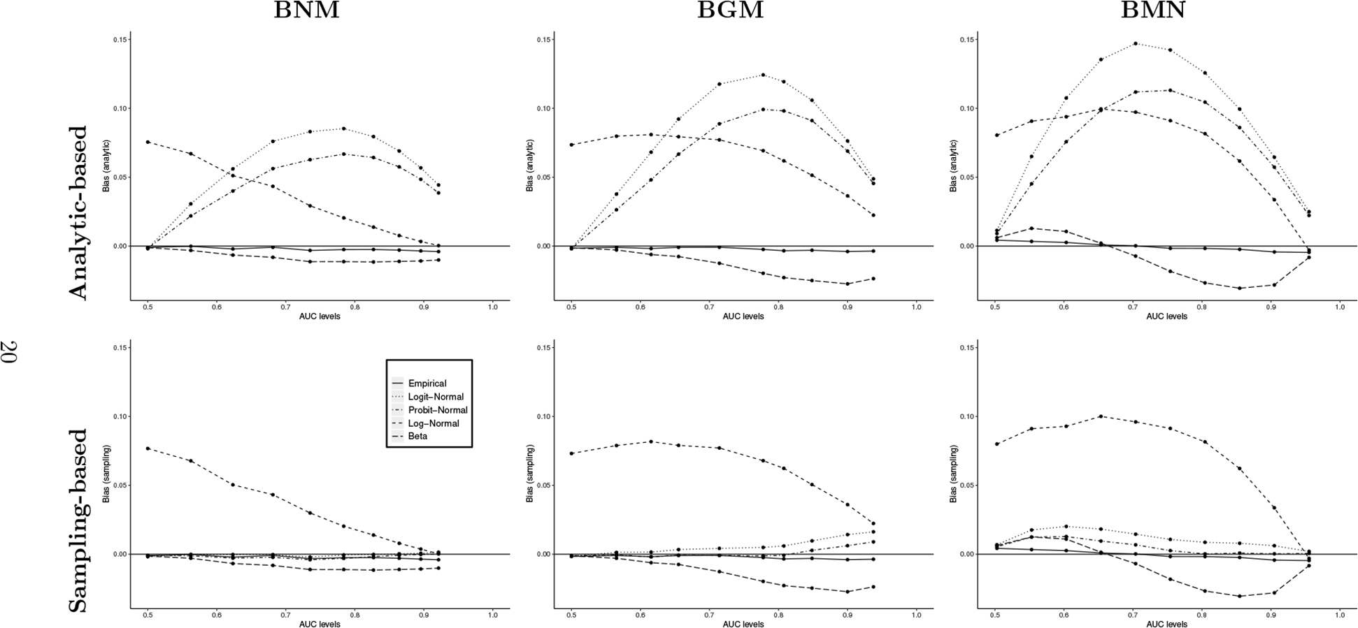
Biases of AUC estimates in the simulation study, n = 100.

With the other two fitting models (Log-Normal and Beta), there is virtually no difference in the results between analytic- and sampling-based AUC estimators. This is expected since, contrary to Logit- and Probit-Normal models, the Log-Normal and Beta models do not involve approximations in analytic-based estimators. The Log-Normal model has poor performance in all situations, except probably at very high AUCs. The high biases (as much as 0.1) essentially renders it useless in practice. The fact that a Log-Normal distribution models a random variable unbounded from the above is the likely culprit. Interestingly, although it operates on the same scale of the data (i.e., no need to transform placement values), the Beta model exhibits larger biases than the duo of Logit/Probit-models. It still performs much better than the Log-Normal model. Finally, when using the PV sample mean to estimate AUC (“Empirical”), the biases are small. Similar findings are noted in Tables 2 and 3 where sample sizes of 200 and 400 are used.

Table 2:

Simulation results of AUCs, n = 200. Bias^s and Bias^a are Sampling- and Analytic-based AUC estimators, respectively, and MESE is mean estimated standard errors.

	True AUC	Empirical		Beta			Log-Normal			Logit-Normal			Probit-Normal
		Bias a	MESE	Bias s	Bias a	MESE	Bias s	Bias a	MESE	Bias s	Bias a	MESE	Bias s	Bias a	MESE
BNM	0.500	0.001	0.0203	0.001	0.001	0.0192	0.087	0.087	0.0473	0.001	0.002	0.0306	0.002	0.002	0.0274
	0.562	−0.001	0.0201	−0.003	−0.003	0.0190	0.073	0.073	0.0438	0.000	0.032	0.0296	−0.001	0.023	0.0268
	0.623	−0.001	0.0195	−0.005	−0.005	0.0185	0.059	0.059	0.0396	0.001	0.062	0.0268	−0.001	0.044	0.0248
	0.681	0.000	0.0185	−0.006	−0.006	0.0175	0.046	0.045	0.0351	0.002	0.083	0.0226	−0.001	0.061	0.0219
	0.735	−0.001	0.0173	−0.009	−0.009	0.0163	0.035	0.034	0.0312	0.001	0.092	0.0181	−0.002	0.069	0.0184
	0.784	−0.001	0.0158	−0.009	−0.009	0.0148	0.023	0.024	0.0268	0.001	0.093	0.0138	−0.001	0.073	0.0148
	0.827	−0.001	0.0142	−0.009	−0.010	0.0131	0.016	0.015	0.0229	0.000	0.087	0.0101	0.000	0.070	0.0114
	0.864	−0.002	0.0125	−0.010	−0.010	0.0112	0.010	0.010	0.0193	0.000	0.076	0.0071	0.001	0.064	0.0084
	0.896	−0.001	0.0107	−0.008	−0.008	0.0093	0.005	0.005	0.0157	0.002	0.064	0.0049	0.003	0.055	0.0060
	0.921	−0.002	0.0091	−0.008	−0.008	0.0076	0.002	0.002	0.0130	0.002	0.050	0.0034	0.003	0.044	0.0042
BGM	0.500	0.000	0.0203	−0.001	0.000	0.0192	0.086	0.086	0.0475	0.000	0.000	0.0307	0.000	0.000	0.0275
	0.565	−0.001	0.0210	−0.002	−0.002	0.0197	0.089	0.089	0.0496	0.002	0.041	0.0321	−0.001	0.028	0.0287
	0.615	−0.001	0.0211	−0.004	−0.004	0.0196	0.093	0.092	0.0505	0.003	0.075	0.0307	−0.001	0.053	0.0282
	0.655	0.000	0.0210	−0.006	−0.006	0.0194	0.090	0.090	0.0498	0.005	0.102	0.0279	0.001	0.073	0.0267
	0.714	−0.001	0.0205	−0.011	−0.011	0.0187	0.084	0.085	0.0485	0.005	0.129	0.0216	0.001	0.097	0.0228
	0.778	−0.002	0.0194	−0.017	−0.017	0.0175	0.074	0.075	0.0455	0.007	0.137	0.0136	0.001	0.109	0.0165
	0.808	−0.002	0.0185	−0.019	−0.019	0.0166	0.069	0.069	0.0431	0.009	0.132	0.0100	0.003	0.110	0.0131
	0.848	−0.002	0.0170	−0.022	−0.022	0.0151	0.058	0.058	0.0390	0.012	0.116	0.0061	0.006	0.101	0.0087
	0.900	−0.002	0.0144	−0.024	−0.024	0.0123	0.042	0.042	0.0323	0.019	0.084	0.0026	0.012	0.077	0.0042
	0.938	−0.002	0.0117	−0.022	−0.022	0.0093	0.027	0.026	0.0255	0.021	0.054	0.0012	0.014	0.051	0.0020
BMN	0.503	0.001	0.0204	0.002	0.002	0.0193	0.088	0.089	0.0478	0.003	0.006	0.0312	0.002	0.004	0.0278
	0.553	0.001	0.0217	0.013	0.013	0.0204	0.097	0.097	0.0518	0.017	0.068	0.0360	0.012	0.046	0.0316
	0.603	0.002	0.0225	0.013	0.013	0.0206	0.104	0.104	0.0548	0.023	0.120	0.0344	0.015	0.083	0.0317
	0.654	0.002	0.0226	0.007	0.007	0.0203	0.109	0.108	0.0563	0.022	0.152	0.0286	0.014	0.110	0.0289
	0.704	0.001	0.0223	−0.003	−0.003	0.0197	0.107	0.109	0.0565	0.019	0.163	0.0216	0.011	0.124	0.0242
	0.754	0.000	0.0213	−0.013	−0.014	0.0187	0.103	0.102	0.0541	0.016	0.158	0.0150	0.007	0.127	0.0187
	0.804	0.000	0.0197	−0.023	−0.023	0.0172	0.089	0.089	0.0494	0.013	0.138	0.0098	0.005	0.116	0.0132
	0.855	−0.002	0.0173	−0.029	−0.030	0.0150	0.070	0.069	0.0425	0.010	0.108	0.0061	0.003	0.094	0.0086
	0.905	−0.002	0.0135	−0.027	−0.027	0.0115	0.039	0.039	0.0309	0.008	0.071	0.0034	0.004	0.064	0.0048
	0.955	−0.002	0.0063	−0.006	−0.006	0.0047	0.000	−0.001	0.0084	0.004	0.030	0.0017	0.004	0.027	0.0021

The results regarding ROC curve estimation are reported in Figures 2–4 for the three sample sizes respectively. Similar to what we observe in AUC estimations, both Logit- and Profit-Normal models estimate ROC curves very well and very closely. Log-Normal model has high empirical mean squared errors (EMSE) under all three data generating mechanisms, especially at low AUC levels. Beta model has satisfactory performance under Bi-Normal data generating mechanism but exhibits elevated EMSEs under the other two, more pronounced at high AUCs.

Figure 2:

Simulation results of ROC curves when the sample size is n = 100. EMSE stands for empirical mean squared error.

Figure 4:

Simulation results of ROC curves when the sample size is n = 400. EMSE stands for empirical mean squared error.

Overall, the simulation study findings are as follows:

1. Log-Normal model is consistently worse than the other models. The large biases make theuse of it questionable in any practice.

2. Probit- and Logit-Normal models perform the best when sampling-based AUC estimatorsare used. The bootstrap approach can be used to obtain a standard error measure.

3. The Beta model has reasonable performance overall, but still fares worse than Probit- or Logit-Normal models. It does produce a standard error without bootstrap.

4. Applications

For illustration, we analyze data from the Successive Small-for-Gestational Age Births Study (Bakketeig et al., 1993) that investigated abnormal fetal growth and its risk factors. The study participants consist of 1879 pregnant women who underwent ultrasound examinations during pregnancy at four scheduled weeks of gestation: 17, 25, 33, and 37. Measures from these ultrasound results, including head and abdominal circumferences and femur length of the fetus, were then used to derive the estimated fetal weight (EFW) (Hadlock et al., 1985). At birth, an infant was classified as large-for-gestational age (LGA) if the birth weight is above the 90th percentile for gestational (Bjerkedal and Skjaerven, 1980). In obstetrics, it is of clinical interest to understand the discriminatory ability of EFW at different times of gestation in distinguishing LGA and non-LGA births, as these information can facilitate maternal diet management and aid delivery routes decision, among others.

Using EFW as test score and LGA/non-LGA as diseased/healthy status, we estimate ROC curves and AUCs separately at the four scheduled weeks of gestation. The placement values are first estimated using a normal model of healthy EFWs (with a quad-root transformation) at each gestation, and are then fed to the four models in Section 2 as well as the Empirical approach.

Table 4 contains estimated AUCs while Figure 5 presents the estimated ROC curves. Standard errors in sampling-based AUC estimates are obtained by bootstrap method.

Table 4:

AUC estimates (standard error) of the Scandinavian Study data under different models.

Estimation	Model	Weeks of gestation
		17	25	33	37
Empirical		0.536 (0.0210)	0.663 (0.0202)	0.773 (0.0171)	0.841 (0.0142)
Analytic	Logit Normal	0.579 (0.0360)	0.742 (0.0280)	0.874 (0.0175)	0.940 (0.0106)
	Probit Normal	0.561 (0.0300)	0.719 (0.0256)	0.850 (0.0178)	0.921 (0.0121)
	Log-Normal	0.591 (0.0412)	0.700 (0.0360)	0.787 (0.0254)	0.845 (0.0182)
	Beta	0.548 (0.0205)	0.665 (0.0201)	0.774 (0.0168)	0.844 (0.0142)
Sampling	Logit Normal	0.548 (0.0232)	0.666 (0.0238)	0.770 (0.0187)	0.831 (0.0199)
	Probit Normal	0.543 (0.0211)	0.665 (0.0217)	0.774 (0.0186)	0.842 (0.0162)
	Log-Normal	0.591 (0.0396)	0.700 (0.0297)	0.787 (0.0202)	0.845 (0.0189)
	Beta	0.548 (0.0222)	0.665 (0.0197)	0.774 (0.0176)	0.844 (0.0129)

Figure 5:

Estimated ROC curves of the Scandinavian Study data under different models.

As expected, Log-Normal and Beta models produce almost identical analytic- and sampling-based AUC estimates while Probit- and Logit-Normal models substantially overestimate the AUCs at all four gestation weeks in analytic-based estimates. Focusing on sampling-based results, we see that the estimates are mostly similar between Probit-, Logit-normal and Beta models and are also close to the Empirical ones. Overall, EFWs from ultrasound examinations closer to delivery have higher AUC values. Take the Probit-Normal model as an example. While EFWs at 17 weeks of gestation can barely predict LGA (AUC = .54, se = .021), it has an excellent discriminatory ability at 37 weeks (AUC = .84, se = .016).

5. Discussion

In this paper, we compared several parametric models for analyzing placement values, a relatively new and promising concept for ROC analysis. We found that both normal models based on logit and probit transformation work very well, with Probit-Normal edging out slightly than Logit-Normal. The Beta model works relatively well with slight negative bias in most situations, except when AUC values are high where biases are more noticeable. Log-Normal model performs poorly in all scenarios, except in the trivial cases of very low AUC values. The inferior performance of Log-Normal is probably related to the fact that an unbounded link function is used with a bounded support.

All four models perform the best under the Bi-Normal mechanism and worst under the Bi-Mixture-Normal mechanism. This calls for more robust approaches such as semi- and nonparametric approaches where the parametric distributional assumptions on the error term is relaxed.

The work in this paper focused on the case of no covariates. As the appeal of PV-based approach to ROC analysis lies in its ability to assess covariate effects, a future work is to investigate these models in the context of the regression framework. While we expect that the findings from unadjusted analysis will hold in adjusted analysis, surprises can arise in complicated situations such as when the test scores have censored values.

Although not directly relevant for the purpose of this paper, the estimation of F₀ and hence the placement value Z are an inherent component of a complete analysis of ROC curves. Quantile regression has been suggested in the literature to estimate F₀. Competing approaches and their performances can be evaluated in future studies.

There has been recent interest in ROC surfaces when three ordinal populations are to be classified by test scores (Li et al., 2012; Xiong et al., 2006). The PV-based approach has been extended accordingly (de Carvalho et al., 2018). A future work is to investigate similar models considered in this manuscript when ROC surfaces and volumes under the surface are of interest.

In light of early work in literature on the robustness of the Bi-Normal model (Hanley, 1988, 1996; Swets, 1986), our simulation study findings are not surprising. However, the PV-based approach expands alternative models (e.g., the Beta model) and provides a platform to consider model robustness in the presence of covariates in future work. Moreover, some of our findings, especially the less than ideal performance of both normal models in select range of AUCs when data are generated from Bi-Gamma and Bi-Mixture-Normal models (Figure 5), suggest a need of further investigation.

Figure 3:

Simulation results of ROC curves when the sample size is n = 200. EMSE stands for empirical mean squared error.

References

- Alonzo T and Pepe M (2002). Distribution-free ROC analysis using binary regression techniques. Biostatistics, 3(3):421–432. [DOI] [PubMed] [Google Scholar]
- Bakketeig L, Jacobsen G, Hoffman H, Lindmark G, Bergsjo P, Molne K, and Rodsten J (1993). Prepregnancy risk-factors of small-for-gestational-age births among parous women in scandinavia. Acta Obstetricia et Gynecologica Scandinavica, 72(4):273–279. [DOI] [PubMed] [Google Scholar]
- Bandos AI, Guo B, and Gur D (2017). Estimating the area under ROC curve when the fitted binormal curves demonstrate improper shape. Academic Radiology, 24(2):209–219. [DOI] [PMC free article] [PubMed] [Google Scholar]
- Bjerkedal T and Skjaerven R (1980). Percentiles of birth weight and crown-heel length for single live births. Tidsskrift for den Norke Laegeforening, 100:1008–1091. [PubMed] [Google Scholar]
- Cai T (2004). Semi-parametric ROC regression analysis with placement values. Biostatistics, 5(1):45–60. [DOI] [PubMed] [Google Scholar]
- Dass SC and Kim SW (2011). Multivariate binormal mixtures for semi-parametric inference on ROC curves. Journal of the Korean Statistical Society, 40(4):397–410. [Google Scholar]
- de Carvalho VI, de Carvalho M, and Branscum A (2018). Bayesian bootstrap inference for the receiver operating characteristic surface. Stat, 7(1):e211. [Google Scholar]
- Dodd L and Pepe M (2003). Semiparametric regression for the area under the receiver operating characteristic curve. Journal of the American Statistical Association, 98(462):409–417. [Google Scholar]
- Dorfman D, Berbaum K, Metz C, Lenth R, Hanley J, and AbuDagga H (1997). Proper receiver operating characteristic analysis: The bigamma model. Academic Radiology, 4(2):138–149. [DOI] [PubMed] [Google Scholar]
- Hadlock F, Harrist R, Sharman R, Deter R, and Park S (1985). Estimation of fetal weight with the use of head, body, and femur measurements - A prospective-study. American Journal of Obstetrics and Gynecology, 151(3):333–337. [DOI] [PubMed] [Google Scholar]
- Hanley J (1988). The robustness of the “Binormal” assumptions used in fitting roc curves. Medical Decision Making, 8:197–203. [DOI] [PubMed] [Google Scholar]
- Hanley J (1996). The use of the “Binormal” model for parametric roc analysis of quantitative diagnostic tests. Statistics in Medicine, 15:1575–85. [DOI] [PubMed] [Google Scholar]
- Hanley J and HajianTilaki K (1997). Sampling variability of nonparametric estimates of the areas under receiver operating characteristic curves: An update. Academic Radiology, 4(1):49–58. [DOI] [PubMed] [Google Scholar]
- Heagerty PJ and Pepe MS (1999). Semiparametric estimation of regression quantiles with application to standardizing weight for height and age in us children. Applied Statistics, 48:533–51. [Google Scholar]
- Li J, Zhou X, and Fine JP (2012). A regression approach to ROC surface, with applications to Alzheimer’s disease. Science China-Mathematics, 55(8):1583–1595. [DOI] [PMC free article] [PubMed] [Google Scholar]
- Metz CE (1986). ROC methodology in radiologic imaging. Investigative Radiology, 21(9):720–733. [DOI] [PubMed] [Google Scholar]
- Pepe M and Cai T (2004). The analysis of placement values for evaluating discriminatory measures. Biometrics, 60(2):528–535. [DOI] [PubMed] [Google Scholar]
- Pepe MS (1997). A regression modelling framework for receiver oerating characteristic curves in medical diagnostic testing. Biometrika, 84:595–608. [Google Scholar]
- Pepe MS (2003). Statistical Evaluation of Medial Tests for Classification and Prediction. Oxford University Press, New York. [Google Scholar]
- Rodriguez-Alvarez MX, Tahoces PG, Cadarso-Suarez C, and Jose Lado M (2011). Comparative study of ROC regression techniques-Applications for the computer-aided diagnostic system in breast cancer detection. Computational Statistics & Data Analysis, 55(1):888–902. [Google Scholar]
- Stanley S and Tubbs J (2018). Beta regression for modeling a covariate adjusted ROC. Science Journal of Applied Mathematics and Statistics, 6(4):110–118. [Google Scholar]
- Swets JA (1986). Indices of discrimination or diagnostic accuracy: their rocs and implied models. Psychological Bulletin, 99:100–17. [PubMed] [Google Scholar]
- Xiong C, van Belle G, Miller J, and Morris J (2006). Measuring and estimating diagnostic accuracy when there are three ordinal diagnostic groups. Statistics in Medicine, 25(7):1251–1273. [DOI] [PubMed] [Google Scholar]
- Zhou X, McClish DK, and Obuchowski N (2002). Statistical Methods in Diagnostic Medicine. Wiley, New York. [Google Scholar]