Partial correlation coefficient for a study with repeated measurements

Abstract

Repeated data are increasingly collected in studies to investigate the trajectory of change in measurements over time. Determining a link between one repeated measurement with another that is considered as the biomarker for disease progression, may provide a new target for drug development. When a third variable is associated with one of the two measurements, partial correlation after eliminating the effect of that variable is able to provide reliable estimate for association as compared to the existing raw correlation for repeated data. We propose using linear regression models to compute residuals by modeling a relationship between each measurement and a third variable. The computed residuals are then used in a linear mixed model (implemented by SAS Proc Mixed) to compute partial correlation for repeated data. Alternatively, the partial correlation may be computed as the average of partial correlations at each visit. We provide two real examples to illustrate the application of the proposed partial correlation, and conduct extensive numerical studies to compare the proposed partial correlation coefficients.

1. Introduction

Executive dysfunction plays an important role in memory deficits in neurodegenerative diseases (Parkinson’s Disease (PD), and Alzheimer’s Disease (AD)) [1, 2, 3]. Executive functions are found to be associated with learning impairments [4]. Cross-sectional studies traditionally use Pearson correlation coefficient to estimate the association between these measurements, such as executive function measurements and learning measurements [5, 6, 7].

In clinical research studies, each patient is often followed over time during the course of a clinical trial to study the change in measurements [8, 9, 10]. Such longitudinal studies provide us with more information regarding the course of the symptoms within chronic diseases. For example, the Parkinson’s Progression Markers Initiative (PPMI) study is a multi-site study aiming at determining progression markers in PD by collecting data from each participant for several years. Recently, Bayram et al. [11] studied the association between repeated cognition, mood and dopaminergic binding measurements in PD using the PPMI database. The traditionally used Pearson correlation coefficient may not be appropriate in a longitudinal study due to the dependence of observations within each participant.

For a study with repeated measurements, Bland and Altman [12, 13] were among the first to study the correlation for repeated data. In their approaches, they used analysis of covariance to control for the subject effect. We refer correlation for repeated data as the raw correlation in the presence of repeated measures. Later, Lam et al. [14] developed a framework to calculate raw correlation based on mixed model under the assumption of a compound symmetry covariance structure for repeated measurements, and Hamlett et al. [15] developed SAS codes for raw correlation calculation. Roy [16] then studied a difference covariance structure, AR(1). In the study reported by Bayram et al. [11], raw correlations with repeated measurements were calculated by using the SAS macros developed by Hamlett et al. [15] and Irimata et al. [17] based on the method proposed by Lam et al. [14].

Previous studies have shown associations between motor impairment (.Unified Parkinson’s Disease Rating Scale Part III scores (UPDRS-III)). and both executive functions and verbal learning in PD [18]. When a third variable is associated with either of the two repeated measurements, partial correlation for repeated measurements after controlling for that variable should be computed and reported [19, 20]. Partial correlation is more likely to produce a reliable estimate for association between two measurements. In partial correlation calculation, we first compute residuals of the repeated measurements after adjusting for a third variable. Then we use these repeated residuals to compute partial correlation. We propose using linear regression models to compute residuals to avoid the model over-fitting issue when a linear mixed model (LMM) with the same covariance structure is used twice to compute both residuals and correlation coefficient. Alternatively, the partial correlation may be computed as the average of partial correlations at each visit. We conduct extensive numerical studies to study the performance of the proposed partial correlation coefficient.

We organize this article as follows. In Section 2, we first briefly introduce the LMM method to compute raw correlation coefficient for repeated measurements, then propose a new method to calculate partial correlation coefficient after controlling for a third variable that is associated with these measurements. In Section 3, we illustrate the application of the proposed partial correlation with two real examples, followed by extensive numerical studies. Lastly, we provide some comments in Section 4.

2. Methods

In contemporary clinical trials, it is very common that a study follows patients for a period of time, sometimes lasting many years. During the follow-up, patients are assessed repeatedly as scheduled, e.g., yearly visit. Suppose a trial has n patients and the number of visits for the i-th patient are m_i, i = 1, 2, ⋯, n. Let two repeated measurements U_ij and W_ij be the j-th observations from the i-th participant, j = 1, 2, ⋯, m_i. The parameter of interest is the correlation between U and W.

2.1. Raw correlation for two repeated measurements

Lam et al. [14] were among the first to propose using linear mixed model to calculate raw correlation coefficient for repeated data under the assumption of a compound symmetry (CS) covariance structure for repeated measurements.

Let $Y_i=\left(U_{i1},W_{i1},U_{i2},W_{i2},\cdots ,U_{i{m}_i},W_{i{m}_i}\right)$ be the vector of observations from the i-th participant, with the vector length of 2m_i.

The LMM statistical model is presented as

$$Y_i=X_i\beta +Z_i{b}_i+{ò}_i,$$

where X_i abd Z_i are the design matrices for the fixed effect and the random effect, respectively. The fixed effect is β = (β₀, β_U, β_W)′, where β₀ is the intercept, and β_U and β_W are the fixed effects of U and W, respectively. Then, the design matrix X_i is a 2m_i × 3 matrix, which is presented as

$$X_i={\left(\begin{array}{ccc}1& 1& 0\\ 1& 0& 1\\ .& .& .\\ 1& 1& 0\\ 1& 0& 1\end{array}\right)}_{2m_i\times 3},$$

where the first column referents the intercept, the second column is for the fixed effect U, and the last column is for the fixed effect W.

Following Lam et al. [14], correlation between U_ij and W_ij is independent of visit:

$$\mathit{\text{Corr}}\left(U_{ij},W_{ij}\right)={\rho }_{UW}.$$

Under a CS covariance structure, two parameters in the covariance structure are: correlation within U as Corr(U_ij, U_ij′) = ρ_U, and the correlation within W as Corr(W_ij, W_ij′ = ρ_W. In addition, correlation between U and W at different visits is Corr(U_ij, W_ij′) = δρ_UW. It is assumed that Corr(U_ij, W_ij′) is often less than Corr(U_ij, W_ij′), which leads to δ < 1. Therefore, the variance covariance matrix for Y_i is calculated as

$$V_i=\mathit{\text{cov}}\left(Y_i\right)={\left(\begin{array}{ccccc}{\sigma }_U^2& {\sigma }_{UW}& \cdots & {\sigma }_U^2{\rho }_U& {\sigma }_{UW}\delta \\ {\sigma }_{UW}& {\sigma }_W^2& \cdots & {\sigma }_{UW}\delta & {\sigma }_W^2{\rho }_W\\ {\sigma }_U^2{\rho }_U& {\sigma }_{UW}\delta & \cdots & {\sigma }_U^2{\rho }_U& {\sigma }_{UW}\delta \\ {\sigma }_{UW}\delta & {\sigma }_W^2{\rho }_W& \cdots & {\sigma }_{UW}\delta & {\sigma }_W^2{\rho }_W\\ \cdots & \cdots & \cdots & \cdots & \cdots \\ {\sigma }_U^2{\rho }_U& {\sigma }_{UW}\delta & \cdots & {\sigma }_U^2& {\sigma }_{UW}\\ {\sigma }_{UW}\delta & {\sigma }_W^2{\rho }_W& \cdots & {\sigma }_{UW}& {\sigma }_W^2\end{array}\right)}_{2m_i\times 2m_i},$$ (1)

where ${\rho }_U^2$ and ${\rho }_W^2$ are the variances of U and W, respectively. The variance covariance matrix can be obtained by using the RANDOM statement and the REPEATED statement in the LMM (e.g., Proc Mixed in SAS). More details on using these two statements in computing raw correlation for repeated data may be found in Hamlett et al. [15] and Irimata et al. [17].

2.2. Partial correlation coefficient for two repeated measurements

When two repeated measurements have a relationship with a third variable (e.g., disease progression in PD may be associated with executive function and verbal learning), partial correlation coefficient between two repeated measurements after controlling for a third variable or a set of variables, is more practically relevant than raw correlation to produce a reliable correlation estimate.

In a cross sectional study, a linear regression model is used to fit each measurement on a third variable, and the residuals from these two separate regression models are used to compute partial correlation coefficient. In a study with repeated measurements, residuals may be computed by fitting a LMM with each measurement as the outcome, and a third variable as the predictor. Then, the computed residuals from the two LMMs are used as the outcome in a LMM as described in the previous subsection to compute partial correlation coefficient. As the same model structure is used twice, the first two LMMs may already remove or partially remove the variation of two measurements from the computed residuals, which leads to the estimate variance being zero in the last LMM.

To overcome the model over-fitting issue, we propose using a simple linear regression model to compute residuals in two steps. In the first step, the baseline measurements are used as outcome in a simple linear regression model with a third variable (G) as the predictor:

$$U_{i1}={\alpha }_{U1}+{\beta }_{U1}{G}_{i1},$$

and

$$W_{i1}={\alpha }_{W1}+{\beta }_{W1}{G}_{i1},$$

where G_i1 is the third variable of the i-th participant at baseline. Suppose a_U1, b_U1, a_W1, and b_W1 are the estimates for α_U1, β_U1, α_W1, and β_W1, respectively. In the second step, the intercept and slope estimates from the fitted models in the first step are then used to compute the predicted value for the measurements at each visit:

$${\widehat{U}}_{ij}=a_{U1}+b_{U1}{G}_{ij},$$

and

$${\widehat{W}}_{ij}=a_{W1}+b_{W1}{G}_{ij},$$

where i = 1, 2, ⋯, n, and j = 1, 2, ⋯, m_i. It follows that the residuals at each visit are computed as.

$$e_{ij}(U)=U_{ij}-{\widehat{U}}_{ij},$$

and

$$e_{ij}(W)=W_{ij}-{\widehat{W}}_{ij}.$$

As suggested by one of the reviewers, residuals can be alternatively computed from the fitted regression models using data at each visit, with the simple linear regression models at the j-th visit as:

$$U_{ij}={\alpha }_{Uj}+{\beta }_{Uj}{G}_{ij},$$

and

$$W_{ij}={\alpha }_{Wj}+{\beta }_{Wj}{G}_{ij}.$$

In this approach, the total number of linear regression models is 2 × max{m_i, i = 1, 2, ⋯, n}, as compared to two regression models in the aforementioned approach by using baseline visit. It should be noted that a study with missing data at later visits would reduce the number of sample size in the regression models that could affect the residual estimates.

2.3. Dependent assumption

The calculated residuals are the outcomes after eliminating the effect of G. Let

$$E_i=\left(e_{i1}\left(U\right),e_{i1}\left(W\right),e_{i2}\left(U\right),e_{i2}\left(W\right),\cdots ,e_{i{m}_i}\left(U\right),e_{i{m}_i}\left(W\right)\right)$$

be the residual vector of Y_i after controlling for a third variable. We then use E_i to replace Y_i in the subsection 2.1 to compute the variance covariance matrix by fitting a LMM. Partial correlation coefficient between U and W after controlling for a third variable G can be computed as

$$\rho =\frac{{\sigma }_{UW}\left(E\right)}{\sqrt{{\sigma }_U^2\left(E\right){\sigma }_W^2\left(E\right)}},$$

where σ_UW(E), ${\sigma }_U^2\left(E\right)$, and ${\sigma }_W^2\left(E\right)$ can be found from the estimated variance covariance matrix of V_i(E), and E represents that these variance, covariance, and partial correlation are computed by using residuals e_i as outcomes.

We refer to the partial correlation under the dependent assumption with residuals computed from baseline regression models or regression models for each visit as ρ_Db and ρ_De, respectively. The difference between them lies on the data used in linear regression models.

2.4. Independent assumption

As suggested by the reviewers, we also include the average of correlations across all visits in this articles. The computed residuals are used to compute correlations at each visit, and the simple average of these correlations are the correlation under the independent assumption that ignore the repeated nature of such data. We use ρ_Ib and ρ_Ie for the partial correlation under independent assumption for residuals computed from linear regression models using baseline data and data at each visit, respectively. We compare these four partial correlations (ρ_Ib, ρ_Ie, ρ_Db and ρ_De) in the following section.

3. Results

We first use two real examples to illustrate the application of the proposed partial correlation coefficient. The first example is from a study to test association between blood-gas analysis and intramural pH from critically ill patients. This example has been frequently used to illustrate the application of correlation for repeated measurements [12, 13, 15, 16]. The second example is from the PPMI database to study correlation between executive function and verbal learning.

3.1. Examples

The first example is from a study with repeated measurements to test the association between blood-gas analysis and intramural pH from critically ill patients enrolled in intensive care units [21]. Data of eight patients from that study are presented in Table 1. The measurements of pH and PaCO₂ are available from Bland and Altman [22], and age of these patients are obtained from the article by Boyd et al. [21]. We identify age by matching the baseline pH measurement from Boyd et al. [21] and that from Bland and Altman [22].

Table 1.

Data for intramural pH and PaCO₂ in a longitudinal correlation study.

Patient	pH	PaCO2	Age	Patient	pH	PaCO2	Age	Patient	pH	PaCO2	Age
1	6.68	3.97	81	4	7.36	5.67	67	6	7.38	4.78	54
1	6.53	4.12	81	4	7.33	5.10	67	6	7.30	4.73	54
1	6.43	4.09	81	4	7.29	5.53	67	6	7.29	5.12	54
1	6.33	3.97	81	4	7.30	4.75	67	6	7.33	4.93	54
2	6.85	5.27	69	4	7.35	5.51	67	6	7.31	5.03	54
2	7.06	5.37	69	5	7.35	4.28	62	6	7.33	4.93	54
2	7.13	5.41	69	5	7.30	4.44	62	7	6.86	6.85	62
2	7.17	5.44	69	5	7.30	4.32	62	7	6.94	6.44	62
3	7.40	5.67	73	5	7.37	3.23	62	7	6.92	6.52	62
3	7.42	3.64	73	5	7.27	4.46	62	8	7.19	5.28	73
3	7.41	4.32	73	5	7.28	4.72	62	8	7.29	4.56	73
3	7.37	4.73	73	5	7.32	4.75	62	8	7.21	4.34	73
3	7.34	4.96	73	5	7.32	4.99	62	8	7.25	4.32	73
3	7.35	5.04	73					8	7.20	4.41	73
3	7.28	5.22	73					8	7.19	3.69	73
3	7.30	4.82	73					8	6.77	6.09	73
3	7.34	5.07	73					8	6.82	5.58	73

Correlation between pH at baseline and age is −0.46400, and correlation between PaCO₂ at baseline and age is −0.22885, which indicate a relatively strong negative correlation between these two measurements and age. In this data, we only have one patient with 9 visits. For this reason, the residual at the 9th visit is computed by using the fitted regression model from the 8th visit.

After controlling for age, partial correlation coefficients between repeated pH and PaCO₂ are presented in Table 2. As compared to the reported raw correlation with repeated data is −0.0100 [15], ρ_Ib and ρ_Ie under the independent assumption are close to the raw correlation. However, the partial correlations under the dependent assumption ρ_Db and ρ_De indicate that pH and PaCO₂ have a strong negative correlation. The partial correlation ρ_Db is very close to ρ_De. The difference between partial correlations under the dependent assumption and raw correlation is substantial.

Table 2.

Partial correlation between intramural pH and PaCO₂ after controlling for age.

Independent assumption		Dependent assumption
ρIb	ρIe	ρDb	ρDe
−0.0388	0.0193	−0.2388	−0.2460

The second example is from the PPMI study to investigate the association between executive function measures and verbal learning measurements after controlling for Movement Disorders Society-UPDRS Part III (MDS-UPDRS3). In this application, we utilize Semantic Fluency (SF) and Hopkins Verbal Learning Test-Revised total learning (HVLTRN) for executive function and verbal learning, respectively. From the PPMI database, 424 PD patients with the first 5 visits are used in the calculation.

Correlation between SF and MDS-UPDRS3 is calculated as −0.131, while correlation between HVLTLRN and MDS-UPDRS3 is slightly stronger, as −0.212. In this example, the third variable is not a constant as that in the first example. The computed partial correlations are presented in Table 3. The partial correlations between memory and executive functioning after controlling for MDS-UPDRS3, ρ_Db and ρ_De, are 0.0980 and 0.0993, which are slightly lower than the raw correlation coefficient of 0.1064. Our findings support that throughout the disease progression; motor symptoms contribute to both domains as shown by correlations between each measure and MDS-UPDRS3. More interestingly, motor symptoms appear to add on to the relationship between executive function and learning. More severe motor impairment may increase the influence of executive function on learning, leading to more severe cognitive impairments.

Table 3.

Partial correlation between executive function measures and verbal learning measurements after controlling for motor impairment.

Independent assumption		Dependent assumption
ρIb	ρIe	ρDb	ρDe
0.1062	0.1064	0.0980	0.0993

3.2. Simulation studies

We conduct simulation studies to compare the performance of partial correlation with raw correlation for a study with repeated measurements. We use dopaminergic binding ratios in caudate and putamen from the PPMI data to estimate mean and variance covariance matrix in the simulation studies.

From the fitted LMM model to compute raw correlation between repeated caudate and putamen measurements, the parameters of the variance covariance matrix are estimated as

$${\sigma }_U^2=0.3367,{\sigma }_W^2=0.08717,{\rho }_U=0.6980,{\rho }_W=0.6028,{\sigma }_{UW}=0.1713{\rho }_{UW},\text{and}\delta \text{=}0.5609/{\rho }_{UW}.$$

Suppose the primary parameter of interest ρ_UW is 0.3, 0.5, 0.7, and 0.9. For a given ρ_UW, the variance covariance matrix V_i in Equation (1) can be computed by using the parameter estimates. We assume each participant has 4 visits. Thus, the size of V_i is 8 × 8. The mean vector Y_i = (U_i1, W_i1, U_i2, W_i2, U_i3, W_i3, U_i4, W_i4,) is estimated as

$$\mu =\left(1.98,0.84,1.80,0.71,1.70,0.67,1.48,0.56\right).$$

We use an R function mvrnorm from the R library MASS to generate random samples of Y_i’s. The values of ρ_UW are chosen to be 0.3 or above in the simulation because the variance covariance matrix should be positive definite in order to utilize the R function mvrnorm to generate samples. A third variable (e.g, age, MDS-UPDRS3) is simulated to have a given correlation with the average of all measurements (8 measurements in Y_i). We assume that each patient is scheduled to visit a clinic once every year. In our simulation study, we use age as a third variable that follows a normal distribution with a mean of 60 and a standard deviation of 10. The baseline value of age is simulated from the correlation model with the average of all measurements. We refer this correlation to be ρ₃, with a range from −0.8 to 0.8 in the simulation studies.

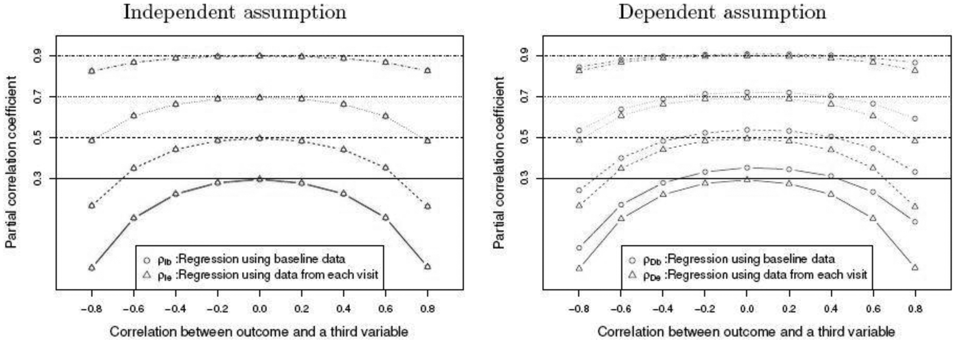
We present the simulated partial correlation coefficients in Figure 1 when sample size is n = 20 and the raw correlation ρ_UW=0.3, 0.5, 0.7, and 0.9. For each configuration, partial correlation coefficient is calculated as the average of 2,000 simulated partial correlation coefficients. It can be seen from the figure that the four partial correlation are much less than the raw correlation ρ_UW, when the correlation |ρ₃| is medium to high. Their difference becomes larger when the pre-specified correlation ρ_UW is medium (e.g, 0.3, 0.5). When a third variable is not correlated with the outcomes (ρ₃ = 0), the partial correlations ρ_De and ρ_Ie using residuals from each visit are generally closer to the raw correlation as compared to the other two partial correlations, ρ_Db and ρ_Ib. When ρ₃ = 0, the true partial correlations should be the same as or at least very close to the raw correlation which is zero. Under this condition, ρ_De and ρ_Ie perform better than the other two correlations. Partial correlation ρ_Db is always larger than ρ_De.

Fig. 1.

Simulated partial correlation between two repeated measurements after controlling for age given the raw correlation between these two measurements from 0.3 to 0.9 when n = 20. Correlations between age and the average of measurements from −0.8 to 0.8 are studied.

Similar results are observed as sample size is increased from n = 20 to n = 60 (see, Figure 2). There is negligible difference between ρ_Ib and ρ_Ie, while the difference for the partial correlations under dependent assumption is still substantial.

Fig. 2.

Simulated partial correlation between two repeated measurements after controlling for age given the raw correlation between these two measurements from 0.3 to 0.9 when n = 60. Correlations between age and the average of measurements from −0.8 to 0.8 are studied.

When the standard deviation of the third variable is increased from 10 to 40 (see, Figure 3), the difference between ρ_De and ρ_Ie becomes bigger. The increasing variation in the third variable would affect the partial correlation estimate. The partial correlations under the independent assumption are very similar to each other for the cases with different standard deviations.

Fig. 3.

Simulated partial correlation between two repeated measurements after controlling for age given the raw correlation between these two measurements from 0.3 to 0.9 when n = 20. Correlations between age and the average of measurements from −0.8 to 0.8 are studied. The standard deviation of age is 10 (left) and 40 (right) under the dependent assumption.

4. Discussion

Partial correlation coefficient for a study with repeated measurements would be proper for use in practice when any third variables are found to be substantially associated with either of the measurements. Although we illustrate the proposed partial correlation methods with two real examples from clinical trials, the developed partial correlations can be applied to other studies. For example, we could apply the proposed methods to compute partial correlation between cost of care and complications after controlling for comorbidities of patients [23, 24].

In this article, we propose using a linear regression model to compute residuals that control for the effect of a third variable under the assumption that the correlation is independent of visit. In a LMM, correlation for each measurement within each participant is assumed to follow a CS covariance matrix structure. Roy [16] considered an AR(1) covariance structure for the repeated measurement. The correlation in the AR(1) structure declines with the distance of visits, while in the CS covariance structure, a constant correlation is assumed. Partial correlation coefficient between memory and executive functioning after controlling for MDS-UPDRS3 is ρ_De = 0.0925 under the AR(1) covariance structure, which is very close to that under the CS covariance structure, ρ_De = 0.0933 in the second example. While, in the first example, the difference between two partial correlation coefficients is substantial: ρ_De = −0.2383 as compared to ρ_De −0.1500 under the AR(1) structure. The choice of covariance matrix (e.g., CS, AR(1), UN) could affect partial correlation calculation in some cases. For that reason, we provide SAS macros that allow users to choose the covariance matrix structure in the calculation. When multiple variables are associated with the two measurements, we would suggest using a multiple linear regression model to calculate residuals [25]. The computed residuals are then used in a LMM to compute partial correlation coefficient [8].

In addition to point estimate for partial correlation coefficient, confidence interval for partial correlation is another important topic. Irimata et al. [17] reviewed several methods to construct confidence interval for raw correlation for repeated measurements and they provided SAS macros for calculation. The delta method can be used to calculate the standard error of the developed partial correlation coefficient [17]. The SAS macros developed by Irimata et al. [17] can be adopted to compute the confidence interval for partial correlation coefficient based on the normal approximation using Fisher’s z transformation. The computed 95% confidence interval based on normal approximation using the SAS macro developed by Irimata et al. [17], is [−0.7484,0.2719] for partial correlation between pH and PaCO₂ after controlling for age in the first example. In addition, bootstrapping is another approach for confidence interval calculation [17].

References

- [1].Cummings JL. Cholinesterase inhibitors for treatment of dementia associated with Parkinson’s disease. Journal of Neurology, Neurosurgery & Psychiatry. 2005;76(7):903–904. [DOI] [PMC free article] [PubMed] [Google Scholar]
- [2].Swanberg MM, Tractenberg RE, Mohs R, Thal LJ, Cummings JL. Executive dysfunction in Alzheimer disease. Archives of Neurology. 2004;61(4):556–560+. [DOI] [PMC free article] [PubMed] [Google Scholar]
- [3].Bondi MW, Kaszniak AW, Bayles KA, Vance KT. Contributions of frontal system dysfunction to memory and perceptual abilities in Parkinson’s disease. Neuropsychology. 1993;7(1):89. [Google Scholar]
- [4].O’Brien TJ, Wadley V, Nicholas AP, Stover NP, Watts R, Griffith HR. The contribution of executive control on verbal-learning impairment in patients with Parkinson’s disease with dementia and Alzheimer’s disease. Archives of clinical neuropsychology: the official journal of the National Academy of Neuropsychologists. 2009. may;24(3):237–244. Available from: http://view.ncbi.nlm.nih.gov/pubmed/19587066. [DOI] [PMC free article] [PubMed] [Google Scholar]
- [5].Bayram E, Banks SJ, Shan G, Kaplan N, Caldwell JZK. Sex Differences in Cognitive Changes in de Novo Parkinson’s Disease. Journal of the International Neuropsychological Society. 2020. feb;26(2):241–249. [DOI] [PMC free article] [PubMed] [Google Scholar]
- [6].Bayram E, Shan G, Cummings JL. Associations between Comorbid TDP-43, Lewy Body Pathology, and Neuropsychiatric Symptoms in Alzheimer’s Disease. Journal of Alzheimer’s Disease. 2019. may;Preprint(Preprint):1–9. Available from: https://www.medra.org/servlet/aliasResolver?alias=iospress&doi=10.3233/JAD-181285. [DOI] [PMC free article] [PubMed] [Google Scholar]
- [7].Zhang H, Shan G. Letter to the Editor: A novel confidence interval for a single proportion in the presence of clustered binary outcome data (SMMR, 2019). SAGE Publications Ltd; 2020. [DOI] [PubMed] [Google Scholar]
- [8].Shan G, Banks S, Miller JB, Ritter A, Bernick C, Lombardo J, et al. Statistical advances in clinical trials and clinical research. Alzheimer’s & Dementia: Translational Research & Clinical Interventions. 2018;4:366–371. [DOI] [PMC free article] [PubMed] [Google Scholar]
- [9].Shan G Two-stage optimal designs based on exact variance for a single-arm trial with survival endpoints. Journal of Biopharmaceutical Statistics. 2020. mar;p. 1–9. Available from: https://www.tandfonline.com/doi/full/10.1080/10543406.2020.1730869. [DOI] [PMC free article] [PubMed] [Google Scholar]
- [10].Shan G Accurate confidence intervals for proportion in studies with clustered binary outcome. Statistical Methods in Medical Research. 2020. apr;p. 096228022091397. Available from: http://journals.sagepub.com/doi/10.1177/0962280220913971. [DOI] [PubMed] [Google Scholar]
- [11].Bayram E, Kaplan N, Shan G, Caldwell JZK. The longitudinal associations between cognition, mood and striatal dopaminergic binding in Parkinson’s Disease. Aging, Neuropsychology, and Cognition. 2019. aug;p. 1–14. [DOI] [PMC free article] [PubMed] [Google Scholar]
- [12].Bland JM, Altman DG. Calculating correlation coefficients with repeated observations: Part 1-Correlation within subjects. BMJ (Clinical research ed). 1995. feb;310(6977):446. Available from: http://www.ncbi.nlm.nih.gov/pubmed/7873953http://www.pubmedcentral.nih.gov/articlerender.fcgi?artid=PMC2548822. [DOI] [PMC free article] [PubMed] [Google Scholar]
- [13].Bland JM, Altman DG. Calculating correlation coefficients with repeated observations: part 2-correlation between subjects. Bmj. 1995;310(6980):446. [DOI] [PMC free article] [PubMed] [Google Scholar]
- [14].Lam M, Webb KA, Donnell. Correlation between two variables in repeated measures. In: PROCEEDINGS-AMERICAN STATISTICAL ASSOCIATION BIOMETRICS SECTION; 1999. p. 213–218. [Google Scholar]
- [15].Hamlett A, Ryan L, Wolfinger R. On the use of PROC MIXED to estimate correlation in the presence of repeated measures. Proc Statistics and Data Analysis. 2004;p. 129–198. [Google Scholar]
- [16].Roy A Estimating correlation coefficient between two variables with repeated observations using mixed effects model. Biometrical journal Biometrische Zeitschrift. 2006. apr;48(2):286–301. Available from: http://view.ncbi.nlm.nih.gov/pubmed/16708779. [DOI] [PubMed] [Google Scholar]
- [17].Irimata K, Wakim P, Li X. Estimation of correlation coefficient in data with repeated measures. In: SAS Paper; 2018. p. 2424. [Google Scholar]
- [18].Wang YXX, Zhao J, Li DKK, Peng F, Wang Y, Yang K, et al. Associations between cognitive impairment and motor dysfunction in Parkinson’s disease. Brain and behavior. 2017. jun;7(6). Available from: http://view.ncbi.nlm.nih.gov/pubmed/28638722. [DOI] [PMC free article] [PubMed] [Google Scholar]
- [19].Shan G Exact confidence limits for the response rate in two-stage designs with over or under enrollment in the second stage. Statistical Methods in Medical Research. 2018. apr;27(4):1045–1055. Available from: http://view.ncbi.nlm.nih.gov/pubmed/27389669. [DOI] [PMC free article] [PubMed] [Google Scholar]
- [20].Jiang T, Cao B, Shan G. Accurate confidence intervals for risk difference in meta-analysis with rare events. BMC medical research methodology. 2020. apr;20(1):98. [DOI] [PMC free article] [PubMed] [Google Scholar]
- [21].Boyd O, Mackay CJ, Lamb G, Bland JM, Grounds RM, Bennett ED. Comparison of clinical information gained from routine blood-gas analysis and from gastric tonometry for intramural pH. Lancet (London, England). 1993. jan;341(8838):142–146. Available from: http://view.ncbi.nlm.nih.gov/pubmed/8093745. [DOI] [PubMed] [Google Scholar]
- [22].Bland JM, Altman DG. Statistics Notes: Correlation, regression, and repeated data. BMJ. 1994;308(6933):896. Available from: https://www.bmj.com/content/308/6933/896. [DOI] [PMC free article] [PubMed] [Google Scholar]
- [23].Shen JJ, Shan G, Kim PC, Yoo JW, Dodge-Francis C, Lee YJ. Trends and Related Factors of Cannabis-Associated Emergency Department Visits in the United States. Journal of Addiction Medicine. 2019. may;13(3):193–200. Available from: http://journals.lww.com/01271255-201906000-00006. [DOI] [PubMed] [Google Scholar]
- [24].Shan G, Gerstenberger S. Fisher’s exact approach for post hoc analysis of a chi-squared test. PLOS ONE. 2017. dec;12(12):e0188709+. Available from: 10.1371/journal.pone.0188709. [DOI] [PMC free article] [PubMed] [Google Scholar]
- [25].Shan G, Bayram E, Caldwell JZK, Miller J, Shen J, Gerstenberger S. Partial correlation coefficient for a study with repeated measurements. Statistics in Biopharmaceutical Research. 2020;p. Revision. [DOI] [PMC free article] [PubMed] [Google Scholar]