

Abstract
The hyperfine coupling between an electron spin and a nuclear spin depends on the Fermi contact coupling aiso and, through dipolar coupling, the distance r between the electron and the nucleus. It is measured with electron–nuclear double resonance (ENDOR) spectroscopy and provides insight into the electronic and spatial structure of paramagnetic centers. The analysis and interpretation of ENDOR spectra is commonly done by ordinary least-squares fitting. As this is an ill-posed, inverse mathematical problem, this is challenging, in particular for spectra that show features from several nuclei or where the hyperfine coupling parameters are distributed. We introduce a novel Tikhonov-type regularization approach that analyzes an experimental ENDOR spectrum in terms of a complete non-parametric distribution over r and aiso. The approach uses a penalty function similar to the cross entropy between the fitted distribution and a Bayesian prior distribution that is derived from density functional theory calculations. Additionally, we show that smoothness regularization, commonly used for a similar purpose in double electron–electron resonance (DEER) spectroscopy, is not suited for ENDOR. We demonstrate that the novel approach is able to identify and quantitate ligand protons with electron–nucleus distances between 4 and 9 Å in a series of vanadyl porphyrin compounds.
Graphical Abstract
ENDOR spectra are analyzed using a non-parametric approach that yields multidimensional distributions of hyperfine coupling parameters. This provides insight into the electronic and geometric structure of spin centers.

1. Introduction
Hyperfine interactions, the magnetic couplings between unpaired electron spins and nearby nuclear spins, provide insight into the spatial distribution of the electron spin density and the geometric structure of paramagnetic spin centers. Hyperfine interactions are probed by high-resolution electron–nuclear double resonance (ENDOR) spectroscopy in solids1 and solutions2,3. ENDOR directly measures nuclear resonance frequencies from which hyperfine couplings are extracted. Among the many pulse ENDOR techniques4, Davies ENDOR5 and Mims ENDOR6 are the two most common. ENDOR is extensively used, often in combination with isotope labeling, to determine the presence of magnetic nuclei near unpaired electron spins7–9, the extent of electron spin density delocalization10–13, and the distance and location of magnetic nuclei relative to an unpaired electron14–19. Electron–nucleus distances of up to 15 Å have been measured20.
The analysis of ENDOR spectra heavily relies on spectral simulation using ordinary least-squares fitting (LSQ) to fit a spin Hamiltonian model to th experimental spectrum. For spin-1/2 nuclei, the hyperfine parameters from this model uniquely determine the ENDOR spectrum, which can be calculated from them in a straightforward fashion. The hyperfine interaction between an electron and a nucleus is represented by a hyperfine tensor that depends on up to six parameters: the isotropic Fermi contact coupling constant aiso, the axial dipolar coupling constant T (which determines the effective distance r), the rhombicity , and three parameters that describe the orientation of the tensor within the spin center. The number of parameters is reduced for nuclei distant from the electron spin density (aiso ≈ 0, ≈ 0) and in the case of non-orientation-selective ENDOR, where the three orientational parameters do not affect the ENDOR spectrum. The hyperfine coupling parameters contain information about the extent to which electron spin density is present at the nucleus, about the effective distance between the nucleus and the delocalized electron, and in orientation-selective situations, the location of the nucleus relative to the delocalized electron spin distribution.
Ordinary LSQ works reasonably well if the ENDOR spectrum contains non-overlapping features of only one or a few magnetic nuclei. It is more challenging for spin centers with many nuclei with overlapping ENDOR signatures and in the presence of substantial spread in the hyperfine couplings due to structural disorder (strain effects). In this case, extracting hyperfine parameters from the spectrum is a mathematically ill-posed problem in the sense that no unique solution exists, and that the solution is extremely sensitive to noise in the data.
A similar problem exists in double electron–electron resonance (DEER) spectroscopy. Like ENDOR, DEER probes magnetic dipolar couplings between pairs of spins, both electrons in this case. Experimental situations in DEER are usually such that contact couplings are negligible, the distances are relatively large, and orientation selection is absent. Therefore, the only coupling parameter that affects the dipolar spectrum is the effective inter-spin distance. In DEER, one common solution to the inversion problem of analyzing the data is Tikhonov regularization21, yielding a distribution of distances r between the two electrons22–25.
Here, we present a novel regularization-based method that analyzes an experimental ENDOR spectrum in terms of a complete non-parametric distribution over hyperfine parameters. We first show that ordinary LSQ fails, and that Tikhonov regularization, widely employed in DEER spectroscopy, is inadequate. We then introduce a regularization approach that augments the LSQ objective function with a penalty term that measures the dissimilarity between the distribution and a prior probability distribution that is obtained from computational-chemistry predictions. This term penalizes regions in hyperfine parameter space that are deemed nonphysical for the molecules under investigation, based on the calculations. We demonstrate and evaluate the method on non-orientation-selective ligand 1H ENDOR spectra of a series of vanadyl porphyrin compounds. These pose a particularly challenging problem, as they have a large number of protons with strongly overlapping ENDOR spectra, as well as protons with significant distributions of hyperfine parameters.
2. The ENDOR spectrum
ENDOR provides a spectrum of nuclear resonance frequencies νn of the spin center. For a spin-1/2 nucleus interacting with a spin-1/2 electron with an isotropic g value, they are26
| (1) |
where , indicates the Euclidean norm, zL is the unit vector along the applied laboratory magnetic field B0, 1 is the 3 × 3 identity matrix, and is the nuclear Larmor frequency, with the nuclear g factor gn, the nuclear Bohr magneton μN, the applied magnetic field magnitude B0, and the Planck constant h.
A is the molecule-fixed hyperfine coupling tensor, in frequency units. It is a 3 × 3 matrix consisting of a sum of two main physical contributions
| (2) |
The first term is the isotropic Fermi contact coupling constant
| (3) |
Here, μ0 is the magnetic constant, μB the Bohr magneton, ge is the electron g value, and is the (positive or negative) electron spin density at R, the location of the nucleus. This term captures the interaction between the nucleus and the electron spin density at its position. The second term in eqn (2) is the dipolar coupling tensor, with elements
| (4) |
where is the electron location, ni and nj are components of the unit vector along the nucleus–electron direction, and δij is the Kronecker delta. This term captures the anisotropic through-space magnetic dipolar coupling of the nucleus with the electron averaged over the electron spin density distribution. Note the inverse-cube dependence on the electron–nucleus distance.
In its principal-axis system, the dipolar tensor is diagonal, and the hyperfine tensor is
| (5) |
where the dipolar coupling constant T describes the strength of the dipolar interaction and the rhombicity parameter quantifies the deviation of from cylindrical symmetry around the n axis.
In this work, we mostly restrict ourselves to the situation where the nucleus and the electron spin density distribution are far enough apart such that the point-dipole approximation holds, i.e. the electron–nucleus distance is much larger than the spread of the spin density. In this case, rhombicity is negligible (), and T becomes
| (6) |
where r is the effective distance between nucleus and electron.
Through eqn (1), the ENDOR spectrum depends on the orientation of the spin center relative to the applied field. The ENDOR spectrum for a powder or frozen-solution sample with a uniform distribution of spin center orientations is the integral of these spectra over all orientations of the spin center. The shape and width of the resulting “powder” spectrum strongly depend on aiso and T.
When using Mims ENDOR to measure the ENDOR spectrum, spectral intensities are subject to a frequency-dependent suppression that depends on τ, the delay between the first two pulses in the Mims ENDOR pulse sequence28. It results in blind spots, i.e. frequencies of maximal suppression, at , where n = 0,1,2,.... This suppression effect is illustrated in Fig. 1a. The Mims ENDOR spectra (color) are overlaid on the unsuppressed ENDOR spectra (dashed, gray lines). The hyperfine parameters used for the simulations are shown in Fig. 1b. The suppression effect has a significant impact on the shape of the ENDOR spectrum; narrow spectra in particular end up resembling pairs of Gaussians due to the central blind spot at ν = νI (n = 0; the ‘hole in the middle’29).
Fig. 1.

(a) Simulated powder Mims ENDOR spectra (colored) of protons with typical axial hyperfine tensors, with τ = 150ns, together with simulated spectra without τ suppression (gray). The shape and the width of the spectrum depend on aiso and T. Spectra are centered around the nuclear Larmor frequency of the proton , were simulated at 344 mT, and are scaled to maximum 1. (b) Hyperfine parameters used for the spectra in (a), in addition to = 0. The top and bottom horizontal axes show the dipolar coupling constant T and the associated effective electron–nucleus distance r. The vertical axes show aiso and the associated contact electron spin density , expressed as a fraction in relation to the contact spin density in a hydrogen atom, ρ0, corresponding to aiso,0 =1420MHz27.
Besides magnetic nuclei that are part of the spin center, ENDOR also reveals interactions with nuclei from the solvent matrix and from other spin centers. These nuclei are spatially uniformly distributed and lead to a narrow peak in the ENDOR spectrum centered at the Larmor frequency that can have significant intensity despite the τ-dependent suppression. The appearance of this matrix peak has been studied in detail30,31, and an excluded-volume model similar to one used in DEER can be applied32. Since all data in this paper were acquired at low concentrations in fully deuterated solvents, the overall proton density is low. Therefore, we model the matrix peak as a Lorentzian
| (7) |
were δ describes the width of the Lorentzian. Other choices of matrix line shapes are possible.
3. Model compounds
We demonstrate our method with the four uncoordinated vanadyl porphyrin compounds shown in Fig. 2a. They all have an identical porphin core with close protons (pyrrole and meso), and differ in the substitution patterns that provide a large number of distant protons. We investigate the effect of meso substituents on the ENDOR spectrum by using vanadyl tetraphenylporphyrin (VO-TPP; no meso protons) and vanadyl diphenylporphyrin (VO-DPP; two meso protons). In vanadyl octaethylporphyrin (VO-OEP) and vanadyl etioporphyrin (VO-EP), the pyrrole protons are all substituted with ethyl groups (VO-OEP) or a mix of methyl and ethyl groups (VO-EP), but the protons at the four meso positions are preserved. The large number of protons with similar small hyperfine couplings makes it particularly challenging to analyze the associated ENDOR spectra.
Fig. 2.
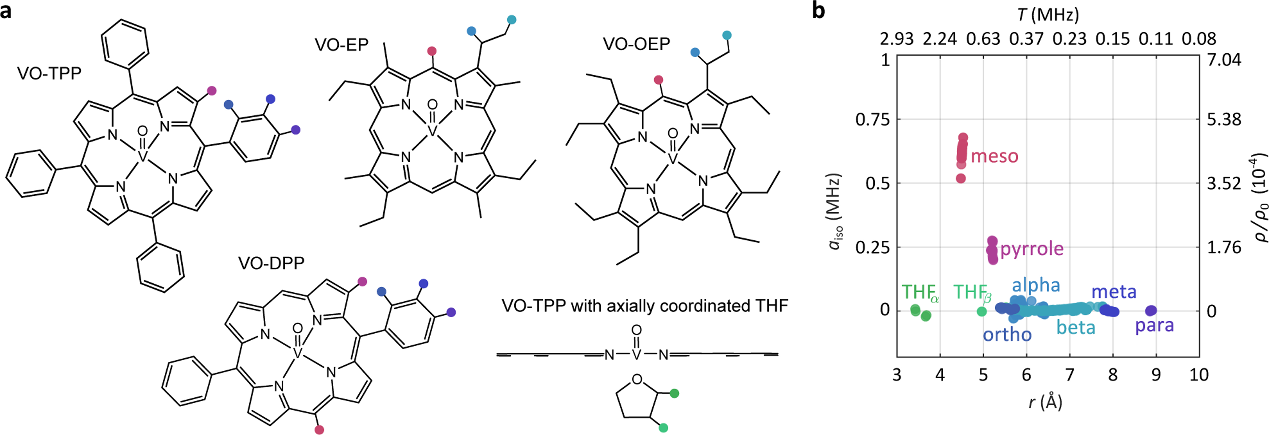
(a) Lewis structures of the four model compounds examined in this study, plus VO-TPP axially coordinated by tetrahydrofuran (THF). The different types of protons are indicated in color. (b) Hyperfine coupling parameters determined from DFT calculations for protons from all structures.
We use density functional theory (DFT) calculations to predict all 1H hyperfine tensors for all five complexes in Fig. 2a. The results are shown in Fig. 2b. Different types of protons appear in distinct regions of the (r,aiso) plane. Protons directly attached to the tetrapyrrole ring (meso and pyrrole) have non-negligible and positive aiso. In contrast, all protons from aliphatic and aromatic substituents and from the THF ligand have aiso values close to zero, but of either sign. The DFT calculations also predict that all proton hyperfine tensors are essentially axial, with ≈ 0.07 for the meso protons and < 0.04 for all others (data not shown). The distinction between protons from THF and ortho protons from VO-TPP and VO-DPP is difficult, as both have aiso close to zero and r in the range of about 5Å. In general, distant protons from larger axial ligands and closer protons on ring substituents are not distinguishable based on aiso and r alone.
4. Ordinary least-squares analysis
The calculation of the ENDOR spectrum S(ν) for a given hyperfine parameter distribution is straightforward:
| (8) |
Here, S is the ENDOR spectrum in vector form, and P is the vector form of a histogram representation of discretized over a sufficiently fine grid of r and aiso, i.e. . K is a kernel matrix where column i contains the simulated ENDOR spectrum for the parameter combination . These spectra form the basis functions of the problem. To model the matrix peak, one column is added to K that contains the Lorentzian line from eqn (7), and the P vector is augmented by one element to provide the amplitude of the matrix peak basis function.
Inverting eqn (8) consists of estimating P from the measured spectrum S. One possible approach is to use ordinary least-squares fitting
| (9) |
where P ≥ 0 indicates that all values in the distribution vector must be nonnegative. This constitutes a mathematically ill-posed problem, since the condition number of K is very large (on the order of 1018 in our case). In other words, the set of ENDOR basis spectra in K have very similar shapes and are almost linearly dependent. This is illustrated in Fig. 3, which shows that a spectrum from a proton with medium r and small aiso can be fit by a proton with long r and a wide distribution of aiso. This means small changes in the spectrum (such as noise) can lead to large changes in the fitted distribution, and a measured noisy spectrum may be fit equally well by several different P.
Fig. 3.

Demonstration of linear dependence within the basis set of Mims ENDOR spectra. (a) An anisotropic spectrum (aiso = 0.62MHz, T = 0.64MHz), simulated at B0 = 350mT, is fit accurately by a linear combination of basis spectra with a small dipolar contribution and large variation in contact coupling (aiso = −0.1–1.6MHz, T = 0.079MHz). The resulting superposition (red) reproduces the anisotropic spectrum almost perfectly. The combinations or r and aiso are shown in (b). Color saturation of the dots for the basis spectra indicates relative weights in the linear combination.
Fig. 4a top shows the experimental spectrum of VO-TPP in red and the fitted spectrum obtained using eqn (9) in blue, together with the residual vector. The bottom panel shows the fitted as well as its projections onto the r and aiso dimensions. For reference, the results of the DFT calculations from Fig. 2 are shown as gray circles. The fit to the spectrum is excellent, with the residuals not displaying any noticeable systematic deviations. However, the fitted strongly deviates from the physical predictions obtained from DFT.
Fig. 4.
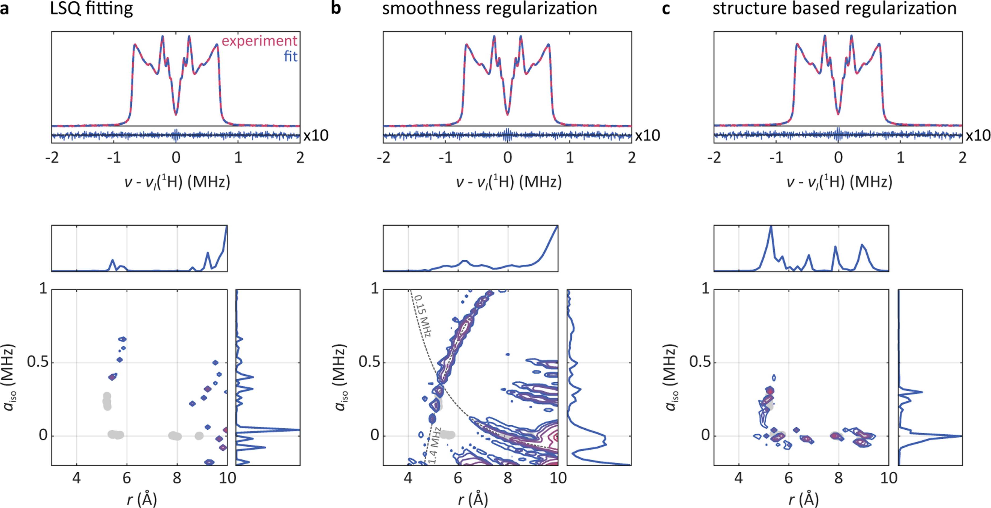
(a) The solution for the ordinary least square fitting approach for VO-TPP, eqn (9). (b) The same data analyzed with smoothness regularization as shown in eqn (11). (c) Regularization with penalty function based on the shown in Fig. 5 and using eqn (12). For (b) and (c) the regularization parameters were selected via the AIC method. The top panels show the experimental spectrum in red and the fit to it in blue, as well as the residuals with a magnification factor of 10. The bottom panels show the density distribution over distance r and contact coupling aiso that was fit to the spectrum, with contour levels at 0.02, 0.05, 0.1, 0.2, 0.5, 0.75, and 0.9 of the distribution maximum. The DFT results for the protons in VO-TPP (pyrrole, ortho, meta, and para) are shown as gray dots. The dotted lines in the lower panel of (b) indicate locations of constant MHz and of constant MHz.
Clearly, the LSQ approach is unsatisfactory. This is a consequence of the severe ill-posedness of the problem. Additional information must be included in the analysis to obtain a unique and stable solution.
5. Regularized least-squares analysis
To include additional information, we use Tikhonov regularization21. This is a well-established method that augments the objective function with a P-dependent quadratic penalty term:
| (10) |
with a regularization operator and a regularization parameter α. This second term helps to stabilize the solution. Various choices for the regularization operator exist: The identity operator minimizes the amplitude of each basis function and avoids spikes in the target distribution. The first and second differential operators can be good choices if the probability distributions are expected to be smooth. Other operators are possible as well.
The regularization parameter α controls the balance between data agreement and regularization; a large value for α prioritizes the regularization and will tolerate a discrepancy between fit and data. What exactly constitutes a large or small value for α depends on the number of data points, the scale of the spectrum, and the regularization operator. Various approaches exist for the selection of an α value, based on various conceptions of optimality33. To select appropriate regularization parameters, we used the Akaike information criterion (AIC)34. For DEER spectroscopy, AIC has been shown to be one of the most reliable selection methods33.
The second term in eqn (10) represents additional information, and from a Bayesian perspective, it represents a prior, i.e. information about the spin center that is available prior to taking the ENDOR spectrum into account.
We examine two choices for . First, we utilize the second derivative, corresponding to a smoothness prior, and show that it does not work. Then, we introduce an operator that calculates the dissimilarity to a physically expected distribution, obtained from structure-based DFT calculations.
5.1. Smoothness regularization
We first examine the use of the second derivative for the regularization operator in eqn (10). This choice is very common in DEER spectroscopy22–25. There, a one-dimensional distance distribution P(r) is fitted to the experimental signal. In contrast, in our case the target distribution is two-dimensional. We therefore include separate regularization terms along the r dimension and the aiso dimensions:
| (11) |
Here, and are matrices representing the second derivative along aiso and r, respectively, and αa and αr are the associated independently selectable regularization parameters.
An analysis of the ENDOR spectrum of VO-TPP using this approach, combined with AIC for the selection of both regularization parameters, is shown in Fig. 4b. The fit to the spectrum is excellent, as in the case of ordinary LSQ. However, the fitted distribution is starkly different. There is significant density at nonphysical combinations of long r and large aiso, inconsistent with the expectations from the DFT calculations (Fig. 2b). Also, the fitted distribution in Fig. 4b shows extended ridges. The more vertical ridge runs along locations of constant MHz and corresponds to a set of spectra with equal overall width (see Fig. 1a). Peaks at some locations along this ridge are also visible in the LSQ fit. The more horizontal ridge runs along locations of constant MHz. The associated set of spectra have identical locations of their inner peaks (see Fig. 1a). Both ridges are a consequence of the smoothness requirement imposed by the second term in eqn (11). Varying αr and αa or using the identity or the first derivative as regularization operators does not improve the situation.
The reason this approach fails is that the added requirement of smoothness along the r and aiso dimensions is not entirely physical. While it might be reasonable to expect some distribution of aiso for the meso protons as a result of structural flexibility of the molecule, the distribution of aiso for more distant protons is expected to be much narrower. Imposing a uniform smoothness requirement over the entire range of aiso is therefore not representative of the physical expectation. A similar argument holds for distributions along the r dimension, where different nuclei will have vastly different distributions of r, depending on the local structural flexibility in the molecule.
5.2. Structure-based regularization
Since we have information from DFT that enables us to distinguish physical from nonphysical solutions, it is advantageous to incorporate this information directly and quantitatively into the objective function. To do this, we solve the regularized minimization problem
| (12) |
with a regularization operator that penalizes P in (r,aiso) regions that are deemed non-realistic based on structural information from quantum-chemical calculations. One form of that achieves this is the multiplicative operator
| (13) |
where is a probability distribution over r and aiso that captures physical expectations about . Unphysical regions in the domain have small values of and therefore large values of ΓP, and increase the value of the objective function. With this operator, the discretized form of the norm in the regularization term in eqn (12) is
| (14) |
This is similar to the cross entropy35–37 of relative to P, . Although it is possible to use the cross entropy directly as a regularization term, we utilize the squared form to keep the objective function of the general quadratic form in eqn (10).
The distribution for the application case in this paper is shown in Fig. 5. It is constructed using the results from the DFT calculations shown in Fig. 2. Mathematical details are given in the Methods section below. It is designed to have significant amplitude at and near locations of DFT predictions, and very small but non-zero amplitude everywhere else, thereby representing our expectation about P. Significant broadening is added to represent uncertainty that accounts for potential errors in the DFT calculations or the underlying structures. One possible alternative to this structure-based is to completely exclude basis functions from the kernel that lie in physically unrealistic regions, equivalent to setting to zero in these regions. In principle, excluding basis functions could also be applied to the LSQ and smoothness approaches, which is just another way of incorporating additional information. However, a that is non-zero everywhere has a crucial advantage, as it does not categorically exclude any region from being included in the fit. With as defined, the method is able to identify protons with large r and aiso if there is strong evidence for them in the data. In general, it is important to keep diffuse enough not to categorically exclude any region.
Fig. 5.

The probability distribution , overlaid on the results from the DFT calculations (gray). Contour levels are at 0.05, 0.1, 0.2, 0.5, 0.75, and 0.9 of the distribution maximum.
The result of analyzing the VO-TPP spectrum using eqn (12) with AIC-selected regularization parameter αP is shown in Fig. 4c. The fit to the data is as excellent as with the other methods. The fact that all three methods result in excellent fits to the spectra that are more or less identical despite gross differences among the fitted distributions illustrates the strong ill-posedness of the problem and the importance of including additional information via regularization. Importantly, however, now the fitted distribution is more physical: it contains very little intensity outside the expected regions, and extended ridges are absent.
As in any regularization approach, the selection of a value for αP plays an important role. If αP is chosen too small, the effect of regularization is reduced, leading to density in areas of nonphysical . On the other hand, large values of αP lead to Pfit with very narrow spikes at some of the maxima of the prior probability function .
6. Results for all compounds
The results for the analysis of all four model compounds are shown in Fig. 6. All ENDOR spectra are fitted very accurately, with all residual vectors showing no significant systematic deviations from zero. All fitted hyperfine distributions are physically reasonable. The method recovers the expected hyperfine couplings well for all investigated compounds: it correctly determines that meso protons are absent in VO-TPP and present in all other complexes, and that there are no pyrrole protons in VO-OEP and VO-EP, in contrast to VO-TPP and VO-DPP.
Fig. 6.

Analysis of the four model vanadyl porphyrin compounds, (a) VO-TPP, (b) VO-DPP, (c) VO-OEP, and (d) VO-EP. The top panels show the experimental spectrum in red and the fit to it in blue, as well as the residuals with a magnification factor of 10. The bottom panels show the distance r vs. contact coupling aiso distribution that was fit to the spectrum, with contour levels at 0.02, 0.05, 0.1, 0.2, 0.5, 0.75, and 0.9 of the distribution maximum, as well as its projections along aiso and r. Results from the DFT simulations for protons of the same type as in the individual compounds are shown as gray dots.
From the contour plots of the fitted , it appears that for VO-DPP and VO-OEP the meso protons are barely present. This is due to the broad distribution of aiso values for these protons. This manifests in the spectra in the form of broad humps in the range between 0.75 to 1.2MHz for VO-DPP and 0.5 to 1.25MHz for VO-OEP and VO-EP. For comparison, the line shape of a meso proton with sharp aiso is shown in Fig. 1a in red. The origin of this distribution is a distribution of ring distortions, which affect the amount of spin density that leaks from the V ion to the meso protons.
Also noticeable in all four cases is non-zero density at slightly negative aiso mostly around 6 Å. DFT calculations indeed predict negative aiso in this area for some of the aliphatic protons (see. Fig. 2). However, VO-TPP only has aromatic protons with aiso very close to zero, which indicates that the experimental spectra do not have sufficient spectral resolution and sensitivity to resolve aiso to less than 0.05 MHz.
VO-OEP and VO-EP show density at aiso ≈ 0 and r ≈ 9 Å, even though there are no protons with these parameters in these compounds. This indicates that the resolving power of ENDOR for these long distances is limited. Two reasons for this are that the associated very narrow spectra have very low intensity due to the suppression of intensity close to νI in Mims ENDOR, and that every other proton contributes intensity around νI as well, leading to spectral congestion. Therefore, the analysis for this region of is unreliable in these examples.
The fitted distributions make it possible to determine the relative abundance of the various types of protons. For this, specific areas of Pfit attributed to each proton type are integrated. The integration areas are based on the 0.05 contour line of and are shown in Fig. 7a using the contour plot of VO-DPP as an example. Probability mass outside of these areas is designated as unassigned.
Fig. 7.
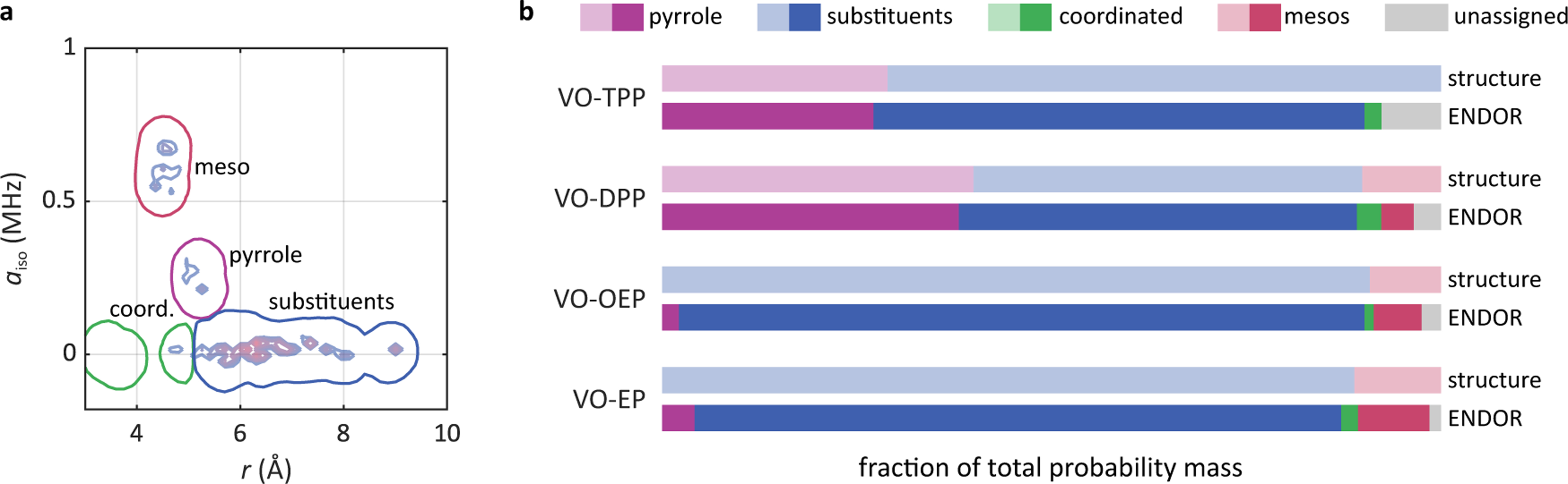
Ligand proton quantitation. (a) Integration areas that were used to calculate the relative abundances of the proton types. For better illustration, the contour plot of Pfit for VO-EP is shown as well. (b) Relative proton abundances for each compound. The upper bar for each compound shows the expected stoichiometric ratios, obtained from the Lewis structure, and the lower bar shows the ones obtained from integration of the fitted hyperfine parameter distribution.
The results of this analysis for all compounds are shown in Fig. 7b. Expected values from the Lewis structures are shown in the upper bar, and integrated intensities obtained from Pfit in the lower bar. Overall, the relative intensities are recovered well, particularly for the pyrrole and substituent protons. About 5–10 % of intensity results unassigned. Meso protons are underestimated most in VO-DPP, where a small fraction is attributed to coordinated protons. Even though the samples did not contain an axial ligand, Fig. 6b shows small values for the area around 4.5 Å. This is due to the fact that protons from axial ligands and the ortho protons from DPP have similar r, as discussed in Sec. 3.
7. Three-dimensional distributions
It is straightforward to extend the approach introduced in this work to situations where the hyperfine tensors can have significant rhombicity . This requires a three-dimensional hyperfine parameter distribution , discretized over a 3D grid such that , and an associated three-dimensional prior, . To demonstrate this, we analyzed VO-EP with a three-dimensional prior, constructed in the same fashion as the 2D prior from the same DFT calculation, but without neglecting . To avoid an explosion of the number of basis functions, it was necessary to halve the kernel resolution along r and aiso.
Figure 8a shows the fit to the spectrum. To visualize , its projections along , aiso, and r are shown in Fig. 8b, c, and d, respectively. The projection along produces a two-dimensional distribution that matches the results from the two-dimensional prior (Fig. 6d) very well. This indicates that the choice of a two-dimensional prior was justified. Analysis of the spectra with the three-dimensional prior yields similar results and in all cases the relative integrals ratios are roughly the same as in the two-dimensional case (data not shown). One significant challenge when going from the 2D to the 3D model is the much larger number of basis functions required in the kernel, resulting in computations with significantly larger memory requirements and slower performance.
Fig. 8.

Analysis of the ENDOR spectrum of VO-EP using a three-dimensional distribution over r, aiso, and the rhombicity parameter . Shown in (a) is the spectrum (red) and the fit (blue) to it, including the residuals. The projection of the fitted three-dimensional distribution P(r,aiso,η) along is displayed in b). Panels c) and d) show the integrals of P(r,aiso,η) along aiso and r, respectively. Contour levels are drawn at 0.02, 0.05, 0.1, 0.2, 0.5, 0.75, and 0.9 of the maximum of the distribution. The DFT results for protons in VO-EP are shown as gray circles. The regularization parameter αP was determined via the AIC method, and 7440 basis functions were used.
8. Discussion and conclusions
In this work we demonstrated a novel approach to qualitatively and quantitatively analyze ENDOR spectra that uses a model based on a two-dimensional hyperfine parameter distribution. We showed that smoothness regularization fails at recovering the correct target distributions. To overcome this, we regularized the problem with a term that penalizes dissimilarity to a prior distribution based on DFT calculations. We demonstrated the method with four model vanadyl porphyrin molecules. The fitted distance vs. contact coupling distributions quantitatively reproduce the spectra and are in good agreement with the physical expectations based on DFT predictions. We also showed that the approach can be extended to extract three-dimensional distributions of distances, contact couplings, and rhombicities. Although demonstrated here for Mims ENDOR only, this method can be applied to other ENDOR experiments (Davies, continuous-wave), as long as the ENDOR line shape for a given hyperfine coupling can be accurately modelled.
The problem discussed here shares the same physical basis as DEER spectroscopy, but several key differences relevant to the analysis exist: (1) In most systems investigated by DEER, contact couplings (exchange couplings) are negligible. This is not the case in ENDOR. Therefore, ENDOR requires a two-dimensional distribution , whereas DEER needs only P(r). (2) In DEER, typically only one other electron spin is significantly coupled to the probed electron spin, whereas in ENDOR there can be many coupled protons. This can lead to significant spectral overlap in ENDOR and aggravates the inversion problem. (3) Whereas in DEER, the dipolar coupling can be distributed due to flexibility of spin labels, in ENDOR it is more often the isotropic coupling that is distributed as a result of structural variability.
We expect distance vs. contact coupling distributions to facilitate analysis and interpretation of ENDOR spectra particularly in difficult cases with significant spectral overlap due to many nuclei in the same distance range and with appreciable hyperfine parameter distributions for some nuclei. One particular application could be the speciation of vanadyl petroporphyrins in crude oil38–41. However, this ENDOR analysis method is applicable to other families of paramagnetic compounds for which DFT calculations can be obtained or where additional information is available that allows the generation of a non-flat prior distribution . The structure-based prior can be extended to include published and validated spectroscopic data from the class of compounds under investigation.
Given that the results show distributions for aiso, in particular for the meso protons of VO-DPP, VO-OEP, and VO-EP, it would be reasonable to include an additional smoothing term for aiso in the objective function. Even though we were able to obtain somewhat smoother results by combining the structure-based regularization with smoothness regularization along aiso and r, in our opinion the benefits are outweighed by the fact that values for one (for smoothing only aiso) or two (smoothing for r and aiso) additional hyperparameters need to be selected. Methods for determination of multiple regularization parameters in a generalized L-curve framework exist42, but it is unclear what the best procedure for regularization parameter selection would be.
As presented, the approach does not allow the determination of the absolute number of protons contributing to the spectrum. To achieve this, the ENDOR amplitude needs to be calibrated, for example via an internal standard. Quantification will be more difficult for protons with small aiso and large r, since the associated narrow ENDOR spectra are very weak due to the suppression hole at ν ≈ νI.
This approach can also be used for orientation-selective ENDOR spectra, or for a set of orientation-selective ENDOR spectra acquired as a function of magnetic field, by utilizing an appropriate kernel K that includes basis functions from a higher-dimensional hyperfine parameter space.
The signal-to-noise ratio plays an important role in the analysis. The structure-based regularization is fairly stable with respect to more elevated noise levels. However, the method starts fitting the noise if the noise is very strong. This will result in spikier distributions.
The structure-based regularization discussed here requires additional knowledge in the form of DFT simulations based on known structures. If the structure of the spin center is unknown, then the approach with still can be used by constructing it such that it represents less specific prior knowledge, for example that it is unlikely to observe a large aiso for long r.
In conclusion, the approach presented here makes congested ENDOR spectra more analyzable, in particular for longer electron–nucleus distances where spectral crowding is typical. However, care must be exercised not to over-interpret the results.
9. Materials and methods
Samples.
All model vanadyl complexes were purchased from Frontier Scientific. The deuterated solvents were obtained from Cambridge Isotope Laboratories. Samples were prepared with ≈1 mM concentration in 1:1 (v/v) toluene-d8/CDCl3, filled into 4mm o.d. quartz tubes and flash-frozen by immersion into liquid nitrogen.
ENDOR.
ENDOR spectra were measured at X-band on a Bruker EleXsys E580 spectrometer with an MD4 probe. For the ENDOR measurements, the magnetic field was set to about 340 mT, so that the microwave was resonant with the mS = −1/2 ↔ +1/2 transition of VO2+. The resonance frequency of this transition is essentially orientation-independent and therefore excludes orientation selection effects41. The temperature was 41–44K. The Mims ENDOR pulse sequence was used with microwave π/2 pulses of 10 ns. The radio frequency π pulse length was 30 μs, to assure narrow-band excitation of the nuclear transitions and prevent power broadening in the ENDOR spectra. We set τ = 150 ns, which puts the first set of suppression points (“blind spots”) with n = ±1 at ±3.3 MHz, outside the spectral range of interest. Before analysis, all spectra were phase corrected, symmetrized, and the amplitude normalized to 1. All measured spectra are provided in the ESI†.
DFT.
DFT calculations were carried out using ORCA 4.1.143,44. The B3LYP45–49 functional was used with the EPR-II50 basis set on all atoms except the vanadium which was modeled with the CP-PPP51 basis set. The integration grid of size 4 was used throughout.
Data analysis.
All data analysis scripts were written in MATLAB and are available in the ESI†. ENDOR basis functions were computed using EasySpin 652 for a 47×61 grid (2867 points) with r ranging from 3 to 9.9 Å with a 0.15 Å step size and aiso ranging from −0.2 to 1 MHz with a 0.02 MHz step size, and a convolutional Gaussian broadening with a full width at half maximum (FWHM) of 30 kHz. The resolution of the kernel was chosen to be high enough to avoid artifacts when fitting a spectrum generated with r, aiso values that fall between two grid points. Suppression envelopes were added according to the experimental parameters. For modeling the matrix peaks, we used a Lorentzian with width δ = 0.32 MHz as per eqn (7). For regularization parameter selection, we used the AIC method25,34. It compares solutions with different regularization parameters by comparing relative amounts of information lost for each and selects the one that retains the most information. The relative abundances of the various proton types were calculated via integration of the fitted distribution Pfit over regions where the prior distribution for that proton had a value of ≥ 0.05 (see Fig. 7a).
Construction of .
We construct as
| (15) |
where is a bi-variate unnormalized Gaussian
| (16) |
where r0,i is the distance (based on the dipolar coupling) and a0,i the contact hyperfine coupling for proton i. Both values are taken directly from the DFT calculations. The widths σr and account for uncertainties in the structure and in the DFT calculations. We used values σr = 0.2Å and = 0.04 MHz.
When choosing the width of the Gaussians it is important to choose them large enough to accommodate for uncertainty of the DFT simulations. If the width is chosen too small the method will provide narrow, potentially spiky distributions, and possibly a bad fit. In contrast, if widths for construction of are chosen too wide, the penalty for unphysical parameter combinations will be too weak and the method will run into similar issues as with least-squares fitting and smoothness regularization.
In eqn (15) we use max instead of a sum for two reasons. First, it allows functions to be placed close to each other without creating unrealistic ridges, e.g. a ridge between the meso and pyrrole protons in Fig. 5b). Second, the amplitudes for all can be set to one, to avoid artificially increasing bias for areas that have a higher density of DFT predictions, such as the region of the aliphatic and aromatic substituents. Other ways of constructing are possible; they are all valid as long they represent the DFT predictions (or any other prior information) acceptably.
For construction of the three-dimensional prior we used a 24×31×10 grid (7440 points) with r ranging from 3 to 9.9 Å with a 0.3 Å step size, aiso ranging from −0.2 to 1 MHz with a 0.04 MHz step size, and ranging from 0 to 0.09 with a 0.01 step size. The prior was constructed in a similar fashion as the two-dimensional one, using tri-variate Gaussians that include the results for from the DFT calculations. For the width along the dimension we used .
Supplementary Material
Acknowledgements
This work was funded by the American Chemical Society Petroleum Research Fund (grant 54860-DNI4), by the National Science Foundation (CHE-1452967), and by the National Institutes of Health (GM125753).
Footnotes
Conflicts of interest
There are no conflicts to declare.
An Electronic Supplementary Information (ESI) is available that contains all experimental data shown in this work, and the MATLAB scripts necessary for analysis.
Notes and references
- 1.Feher G, Physical Review, 1956, 103, 834–835. [Google Scholar]
- 2.Hyde JS and Maki AH, The Journal of Chemical Physics, 1964, 40, 3117–3118. [Google Scholar]
- 3.Hyde JS, The Journal of Chemical Physics, 1965, 43, 1806–1818. [Google Scholar]
- 4.Harmer JR, eMagRes, John Wiley & Sons, Ltd, Chichester, UK, 2016, pp. 1493–1514. [Google Scholar]
- 5.Davies ER, Physics Letters A, 1974, 47, 1–2. [Google Scholar]
- 6.Mims WB, Proceedings of the Royal Society of London. Series A, Mathematical and Physical Sciences, 1965, 283, 452–457. [Google Scholar]
- 7.Nick TU, Lee W, Koßmann S, Neese F, Stubbe J. and Bennati M, Journal of the American Chemical Society, 2015, 137, 289–298. [DOI] [PMC free article] [PubMed] [Google Scholar]
- 8.Rao G, Tao L, Suess DLM and Britt RD, Nature Chemistry, 2018, 10, 555–560. [DOI] [PMC free article] [PubMed] [Google Scholar]
- 9.Rao G, Tao L. and David Britt R, Chemical Science, 2020, 11, 1241–1247. [DOI] [PMC free article] [PubMed] [Google Scholar]
- 10.Scholes CP, Lapidot A, Mascarenhas R, Inubushi T, Isaacson RA and Feher G, Journal of the American Chemical Society, 1982, 104, 2724–2735. [Google Scholar]
- 11.Harmer J, Van Doorslaer S, Gromov I, Bröring M, Jeschke G. and Schweiger A, The Journal of Physical Chemistry B, 2002, 106, 2801–2811. [Google Scholar]
- 12.Baute D. and Goldfarb D, The Journal of Physical Chemistry A, 2005, 109, 7865–7871. [DOI] [PubMed] [Google Scholar]
- 13.Peeks MD, Tait CE, Neuhaus P, Fischer GM, Hoffmann M, Haver R, Cnossen A, Harmer JR, Timmel CR and Anderson HL, Journal of the American Chemical Society, 2017, 139, 10461–10471. [DOI] [PMC free article] [PubMed] [Google Scholar]
- 14.Babcock GT, El-Deeb MK, Sandusky PO, Whittaker MM and Whittaker JW, Journal of the American Chemical Society, 1992, 114, 3727–3734. [Google Scholar]
- 15.Lee H-I, Dexter AF, Fann Y-C, Lakner FJ, Hager LP and Hoffman BM, Journal of the American Chemical Society, 1997, 119, 4059–4069. [Google Scholar]
- 16.Yang TC, Wolfe MD, Neibergall MB, Mekmouche Y, Lipscomb JD and Hoffman BM, Journal of the American Chemical Society, 2003, 125, 7056–7066. [DOI] [PubMed] [Google Scholar]
- 17.Brecht M, van Gastel M, Buhrke T, Friedrich B. and Lubitz W, Journal of the American Chemical Society, 2003, 125, 13075–13083. [DOI] [PubMed] [Google Scholar]
- 18.Horitani M, Offenbacher AR, Carr CAM, Yu T, Hoeke V, Cutsail GE, Hammes-Schiffer S, Klinman JP and Hoffman BM, Journal of the American Chemical Society, 2017, 139, 1984–1997. [DOI] [PMC free article] [PubMed] [Google Scholar]
- 19.Hoeke V, Tociu L, Case DA, Seefeldt LC, Raugei S. and Hoffman BM, Journal of the American Chemical Society, 2019, 141, 11984–11996. [DOI] [PMC free article] [PubMed] [Google Scholar]
- 20.Meyer A, Dechert S, Dey S, Höbartner C. and Bennati M, Angewandte Chemie International Edition, 2020, 59, 373–379. [DOI] [PMC free article] [PubMed] [Google Scholar]
- 21.Tikhonov AN, Doklady akademii nauk, 1963, 151, 501–504. [Google Scholar]
- 22.Bowman MK, Maryasov AG, Kim N. and DeRose VJ, Applied Magnetic Resonance, 2004, 26, 23. [Google Scholar]
- 23.Jeschke G, Panek G, Godt A, Bender A. and Paulsen H, Applied Magnetic Resonance, 2004, 26, 223–244. [Google Scholar]
- 24.Chiang Y-W, Borbat PP and Freed JH, Journal of Magnetic Resonance, 2005, 172, 279–295. [DOI] [PubMed] [Google Scholar]
- 25.Ibáñez L. Fábregas, Jeschke G. and Stoll S, Magnetic Resonance, 2020, 1, 209–224. [DOI] [PMC free article] [PubMed] [Google Scholar]
- 26.Iwasaki M, Journal of Magnetic Resonance (1969), 1974, 16, 417–423. [Google Scholar]
- 27.Karshenboim SG, Physics Reports, 2005, 422, 1–63. [Google Scholar]
- 28.Schweiger A. and Jeschke G, Principles of Pulse Electron Paramagnetic Resonance, Oxford University Press, Oxford, UK; New York, 2002. [Google Scholar]
- 29.Doan PE, Lees NS, Shanmugam M. and Hoffman BM, Applied Magnetic Resonance, 2009, 37, 763. [DOI] [PMC free article] [PubMed] [Google Scholar]
- 30.Dikanov SA, Tsvetkov YD and Astashkin AV, Chemical Physics Letters, 1982, 91, 515–519. [Google Scholar]
- 31.Astashkin AV and Kawamori A, Journal of Magnetic Resonance, 1998, 135, 406–417. [DOI] [PubMed] [Google Scholar]
- 32.Kattnig DR, Reichenwallner J. and Hinderberger D, The Journal of Physical Chemistry B, 2013, 117, 16542–16557. [DOI] [PubMed] [Google Scholar]
- 33.Edwards TH and Stoll S, Journal of Magnetic Resonance, 2018, 288, 58–68. [DOI] [PMC free article] [PubMed] [Google Scholar]
- 34.Akaike H, IEEE Transactions on Automatic Control, 1974, 19, 716–723. [Google Scholar]
- 35.Shannon CE, The Bell System Technical Journal, 1948, 27, 379–423. [Google Scholar]
- 36.Good IJ, Proceedings of the IEE - Part C: Monographs, 1956, 103, 200–204. [Google Scholar]
- 37.Kullback S. and Leibler RA, Annals of Mathematical Statistics, 1951, 22, 79–86. [Google Scholar]
- 38.Goulon J, Retournard A, Friant P, Goulon-Ginet C, Berthe C, Muller J-F, Poncet J-L, Guilard R, Escalier J-C and Neff B, Journal of the Chemical Society, Dalton Transactions, 1984, 0, 1095–1103. [Google Scholar]
- 39.Qian K, Mennito AS, Edwards KE and Ferrughelli DT, Rapid Communications in Mass Spectrometry, 2008, 22, 2153–2160. [DOI] [PubMed] [Google Scholar]
- 40.McKenna AM, Purcell JM, Rodgers RP and Marshall AG, Energy & Fuels, 2009, 23, 2122–2128. [Google Scholar]
- 41.Mannikko D. and Stoll S, Energy & Fuels, 2019, 33, 4237–4243. [Google Scholar]
- 42.Belge M, Kilmer ME and Miller EL, Inverse Problems, 2002, 18, 1161–1183. [Google Scholar]
- 43.Neese F, WIREs Computational Molecular Science, 2012, 2, 73–78. [Google Scholar]
- 44.Neese F, WIREs Computational Molecular Science, 2018, 8, e1327. [Google Scholar]
- 45.Becke AD, Physical Review A, 1988, 38, 3098–3100. [DOI] [PubMed] [Google Scholar]
- 46.Stephens PJ, Devlin FJ, Chabalowski CF and Frisch MJ, The Journal of Physical Chemistry, 1994, 98, 11623–11627. [Google Scholar]
- 47.Lee C, Yang W. and Parr RG, Physical Review B, 1988, 37, 785–789. [DOI] [PubMed] [Google Scholar]
- 48.Becke AD, The Journal of Chemical Physics, 1993, 98, 5648–5652. [Google Scholar]
- 49.Becke AD, The Journal of Chemical Physics, 1993, 98, 1372–1377. [Google Scholar]
- 50.Rega N, Cossi M. and Barone V, The Journal of Chemical Physics, 1996, 105, 11060–11067. [Google Scholar]
- 51.Neese F, Inorganica Chimica Acta, 2002, 337, 181–192. [Google Scholar]
- 52.Stoll S. and Schweiger A, Journal of Magnetic Resonance, 2006, 178, 42–55. [DOI] [PubMed] [Google Scholar]
Associated Data
This section collects any data citations, data availability statements, or supplementary materials included in this article.