First ICON-FUV Nighttime NmF2 and hmF2 Comparison to Ground and Space-Based Measurements

Abstract

The Far Ultra Violet (FUV) ultraviolet imager onboard the NASA-ICON mission is dedicated to the observation and study of the ionosphere dynamics at mid and low latitudes. We compare O⁺ density profiles provided by the ICON FUV instrument during nighttime with electron density profiles measured by the COSMIC-2 constellation (C2) and ground-based ionosondes. Co-located simultaneous observations are compared, covering the period from November 2019 to July 2020, which produces several thousands of coincidences. Manual scaling of ionogram sequences ensures the reliability of the ionosonde profiles, while C2 data are carefully selected using an automatic quality control algorithm. Photoelectron contribution coming from the magnetically conjugated hemisphere is clearly visible in FUV data around solstices and has been filtered out from our analysis. We find that the FUV observations are consistent with the C2 and ionosonde measurements, with an average positive bias lower than 1 × 10¹¹e/m³. When restricting the analysis to cases having an N_mF₂ value larger than 5 × 10¹¹e/m³, FUV provides the peak electron density with a mean difference with C2 of 10%. The peak altitude, also determined from FUV observations, is found to be 15 km above that obtained from C2, and 38 km above the ionosonde value on average.

1. Introduction

On October 11, 2019, NASA’s ICON satellite was launched into a circular orbit at about 590 km altitude, inclined by 27°. The spacecraft carries four scientific instruments dedicated to the study of the coupling between the lower atmosphere, the upper atmosphere, and the solar wind. Besides the in-situ plasma measurement performed by the Ion Velocity Meter (IVM) (Heelis et al., 2017), the remaining three instruments remotely sense the neutral and ionized atmosphere at altitudes ranging from about 90–600 km by observing airglow emissions in several wavelength ranges. In the visible domain, the Michelson Interferometer for Global High-resolution Thermospheric Imaging (MIGHTI) observes the red and green oxygen airglow lines for wind speed retrieval and the O₂ A-band in the near-infrared to measure the thermospheric temperature (Englert et al., 2017; Harding et al., 2017; Stevens et al., 2017). O⁺ density profiles are retrieved at the 12-s measurement cadence by the two complementary instruments operating in the ultraviolet: the Far Ultra Violet Imaging Spectrograph (FUV) and the Extreme Ultra Violet Spectrograph (EUV). The first one simultaneously measures the OI–135.6 nm emission of atomic oxygen and the Lyman-Birge-Hopfield (LBH) band of N₂ near 157 nm (Mende et al., 2017). During nighttime, the 135.6-nm channel is used alone to infer the O⁺ density profile by observing the radiative recombination of oxygen ions with ambient electrons (Kamalabadi et al., 2018). On the dayside, both the 135.6 nm and LBH emissions are measured and combined to determine O and N₂ altitude profiles and column O/N₂, used to monitor the atmospheric composition changes (Stephan et al., 2018). The EUV spectrograph records limb altitude profiles of terrestrial emissions in the extreme ultraviolet spectrum from 54 to 88 nm (Sirk et al., 2017). Specifically, the OII–61.7 and 83.4 nm emissions are used to retrieve daytime O⁺ altitude profiles (Stephan et al., 2017).

The radio-occultation space mission program COSMIC-2 (C2) currently provides up to 3,000 electron density profiles on a daily basis since October 1, 2019, using six spacecraft orbiting above low latitudes at similar altitudes as ICON. Additionally, ground-based ionosondes allow retrieving precise and accurate measurements of the electron density profile up to the peak altitude. These two data sets provide a large and robust database against which we will compare the ICON measurements, for the purpose of determination of relative biases in the data sets when measuring the peak density and its height. In addition, they consist of valuable method-independent data sets as they rely on radio waves, whose propagation in the ionosphere is different from that of airglow ultraviolet emission. Radio observations offer an advantage for this study in that they are weather and illumination conditions independent, so that they are available at any time of day and night. However, the radio-occultation technique does not provide observations at a regular cadence and spacing because it depends on the location where the transmitters are occulting. This is not the case of ICON FUV instrument which provides mostly instantaneous measurements every 12 s along the orbit.

Recently, Bust and Immel (2020) simulated the ingestion of ICON FUV and EUV density profiles into the Ionospheric Data Assimilation Four-Dimensional (IDA4D) assimilative model and demonstrated their improvement by assimilating airglow data in models that already make use of GNSS radio-occultation and ionosonde data. In this framework, it is important to estimate the agreement level between the different data sets to assimilate them while taking into account their differences to minimize any conflicts in the measurements. For instance, it is well known that ionosondes are blind to some density depletions, like the so-called “valley” between the E and F1-layers, as well as to the ionospheric topside. Additionally, depletions due to gravity waves or hidden secondary maxima would not be seen by ionosondes, which is not the case of airglow measurements like those provided by the ICON-FUV instrument. Perfect agreement between airglow data and ionosonde profiles is therefore not expected during the occurrence of significant gravity wave disturbances, for instance. This is the reason why the following study focuses on the peak parameters only, namely N_mF₂ and h_mF₂ for peak density and altitude, respectively. In this study, we provide the first comparison of ICON airglow-derived O⁺ density profiles with ionosonde and C2 electron density profiles during nighttime conditions. First, data are detailed and carefully selected based on strict criteria to ensure a highly reliable study. The methodology for identifying co-located simultaneous observations, called conjunctions, is detailed, in addition to the data quality control. Next, we compare the peak altitude (h_mF₂) and density (N_mF₂) from the different data sets on statistical grounds. Differences are found and discussed, and several research perspectives are drawn for future work.

2. Data and Methodology

The ICON observatory was turned to science mode on November 16, 2019, and the mission has produced FUV data on a daily basis. We analyze therefore the data produced since then.

2.1. Nighttime FUV

The main production mechanism of nighttime OI–135.6 nm photons in the Earth ionosphere is the radiative recombination of O⁺ ions:

$${\text{O}}^{+}+\text{e}\to {\text{O}}^{*}\to \text{O}+hv$$ (1)

with h being the Planck constant and v the radiation frequency. The other production mechanism of OI–135.6 nm photons is the mutual neutralization of atomic oxygen ions O⁺ and O⁻ in the F-region which, according to Qin et al. (2015), can contribute up to 38% of the total nighttime OI–135.6 nm emission. Loss of OI–135.6 nm photons is due to multiple scattering and pure absorption, the latter being the dominant effect below the altitude of 110 km. Radiative recombination, mutual neutralization, pure absorption and resonant scattering are included into the radiative transfer model used to convert brightness measurements into vertical O⁺ density profiles (Kamalabadi et al., 2018). The profile retrieval algorithm consists in minimizing the difference between the forward model and the observations, including a Tikhonov regularization scheme. The forward model simulates the radiative transfer of the 135.6 nm emission by dividing the ionosphere in several spherical layers with boundaries determined by the tangent altitudes and inside which the total volume emissivity is considered as a constant. Solving integrated emission for each line of sight for the electron density profile, which is considered as equal to O⁺ density, is achieved through the Tikhonov quadratic regularization method. The optimal regularization parameter computation is based on the L-curve criterion, ensuring an optimal smooth estimation of the whole O⁺ profile. The FUV inversion algorithm uses the spherical symmetry hypothesis like for a classical Abel inversion. This has to be taken into account when comparing FUV data with external data sources for which inversion is needed: for instance, as discussed in the next section, COSMIC-2 (C2) relies on an improved Abel inversion formulation that accounts for possible gradients based on the climatological maps constructed from previous observations (Chou et al., 2017).

The FUV O⁺ density profiles are enclosed in the ICON mission data product L2.5 which consists of six profiles resulting from the inversion of OI–135.6 nm limb brightness profiles measured in six sections along the horizontal field of view of the imager every 12 s. The processing chain of FUV L2.5 includes calibration and quality control that ensures a precise profile. They include the dynamic background subtraction algorithm, which makes use of an unused region of the FUV detector to characterize the dark current background along the altitude pixels. Another important step of the level-1 to level-2 processing is the implementation of a star-removal algorithm to filter out the bright signal due to stars present in the FUV field of view. In addition to estimates of the O⁺ density profile, the nighttime data product L2.5 comes with a standard error assigned to each of these values. These statistical error values result from detector count rate error propagation implemented into the inversion algorithm. The uncertainties do not reflect model inaccuracies such as possible neutral density mismodeling nor include systematic errors due to the Tikhonov regularization used in the inversion algorithm. We integrate along a line of sight that can be longer than 1,000 km around the limb and thus covers a large region. A large range of geographic locations corresponds therefore to each tangent altitude, so that we need to select one geographic location to compute the distance between other measurements location and that of ICON profiles. Ideally, the reference location of each profile should be located in the region where the maximum contribution to the brightness is expected. In this study, we chose to geolocate the profile at the tangent altitude corresponding to the peak height h_mF₂ deduced from ICON-FUV observation. The version number of L2.5 NetCDF files used for this study is v03 and the revision number corresponds to that of the last file available at the time of writing these lines.

2.2. Ionosonde

The principle of the ionospheric sounding is simple: an emitting antenna sends radio pulses with frequency ranging from 1 to 30 MHz in the vertical direction while another antenna receives the reflected signals. One can therefore compute the travel time of the different pulses, which allows to associate a reflecting height with each frequency. These observations are then presented on a graphical plot called an ionogram, which illustrates the vertical structure of the ionosphere, mainly from the E-region to the F₂-peak. The ionograms actually show the travel time of the pulsed signal, translated in distance units, from the transmitter to the receiver and considering a vertical incidence. As this signal always travels more slowly in the ionosphere and back to the receiver than in free space, the observed altitudes, called virtual heights, always exceed the true reflection heights. An inversion algorithm is therefore needed to retrieve the true heights and derive, for instance, that of the peak, that is, h_mF₂. In the frame of this study, we use the SAO-X software developed by Lowell Digisonde International (LDI), Massachusetts. The manual scaling of ionograms consists in graphically selecting its important features to allow the inversion algorithm to properly retrieve the electron density profile (Piggot & Rawer, 1978). Each ionogram considered in this study has been manually scaled by considering a time sequence of ionograms to help the interpretation and reduce the uncertainty level. The expected precision depends however on both the scaler skill and on the ionogram itself. Indeed, the presence of some features prevents an easy and unambiguous scaling, like the presence of range or frequency spread, a blanketing sporadic E-layer, forked traces due to the presence of tilts or strong absorption. In such cases, the ionogram is declared not suitable for the purpose of this study and discarded from our analysis. However, even considering a perfect, noiseless ionogram, the error on the critical frequency still depends on the scaler’s ability to correctly interpret the ionogram. Under optimal conditions, the uncertainty on the critical frequency f_oF₂ due to user’s pointing and interpretation, or σ_f, can be estimated to about 0.1 MHz, which can be translated in electron density error σ_Ne using error propagation theory by σ_Ne = σ_f f_oF₂/40.25, expressed in e/m³. At last, let us note that, unlike FUV instrument onboard ICON, ionosondes provide the electron density profile N_e instead of the O⁺ density profile, which can be significantly different at low altitudes where other ions such as NO⁺ and ${\text{O}}_2^{+}$ contribute to N_e or in the topside F-region, where H⁺ density becomes significant. It is also worth reminding that ionosondes are not able to sense the ionosphere above the F-peak, so that topside profiles provided by ionosonde measurements are extrapolated values and should not be used in our comparisons. The location of ionosonde stations used in this study is shown in Figure 1.

Figure 1.

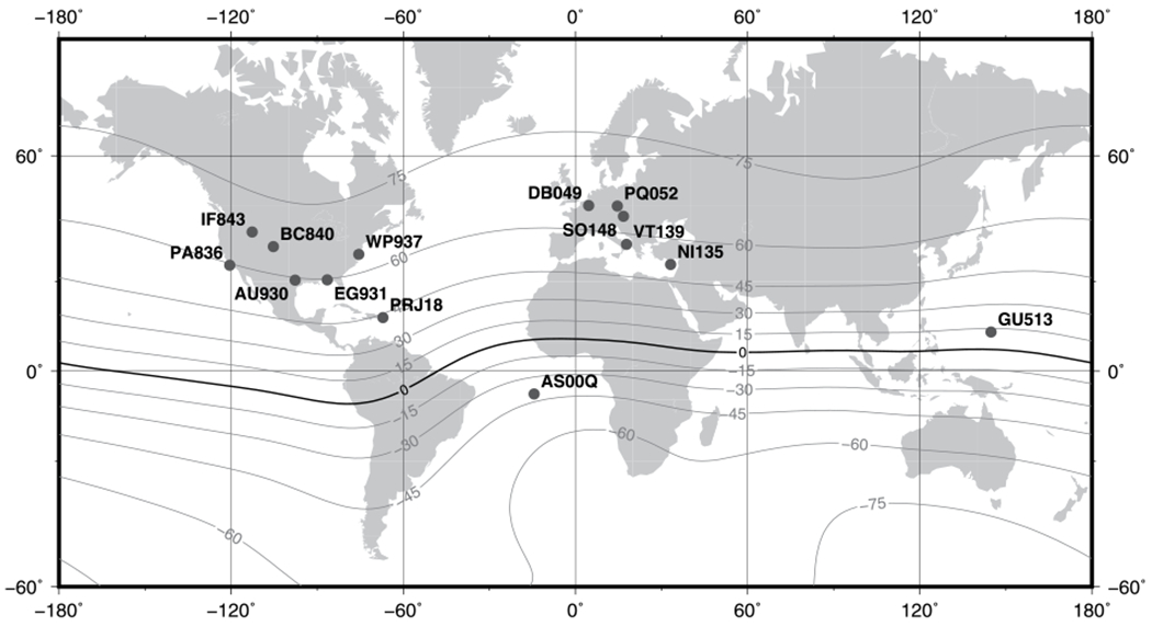
Map of ionosonde stations used in this study. Contour lines correspond to dip inclination derived from the International Geomagnetic Reference Frame (IGRF) 13 (Thébault et al., 2015), expressed in degrees.

2.3. COSMIC-2

The US Air Force Space Test Program successfully launched six FORMOSAT-7/COSMIC-2 (F7C2) satellites into a 24° inclination low Earth orbit on June 25, 2019. The primary F7C2 mission objective is to continuously and uniformly collect atmospheric and ionospheric data to be used as input to daily near real-time weather forecasts, climate studies, and space weather research (Straus et al., 2020). Ionospheric electron density profiles result from the inversion of GNSS Total Electron Content (TEC) observations performed by the COSMIC-2 (C2) spacecraft, assuming a local symmetry of the electron density along the lines of sight (LoS) between the GPS or GLONASS satellites and the C2 spacecraft. As horizontal gradients exist in the ionosphere, and particularly within the equatorial anomaly, this assumption is generally not strictly valid and the retrieved profile corresponds rather to a mapping of the gradients than to an actual vertical profile at the peak location. Therefore, the main error in the electron density profiles retrieval using radio-occultation is due to the assumption of spherical symmetry made by the Abel inversion method, which gives relatively large errors in the low-latitude region and at low altitudes (Yue et al., 2011). Yue et al. (2010) showed that this assumption results in overestimates of the electron density in the north and south of the equatorial ionization anomaly (EIA) crests and underestimates of the electron density surrounding the EIA crests. To take into account the horizontal gradients, recent studies aimed at adding asymmetry factors into the Abel inversion process. The resulting “Ne-aided Abel” inversion method improves the electron density profiles by mitigating the artificial plasma caves and negative electron density in the daytime E-region, in addition to making the F-region EIA crests more distinct (Chou et al., 2017). This algorithm, which provides the COSMIC-2 electron density profiles used in this study, relies on three-dimensional time-dependent electron density measurements based on the climatological maps constructed from previous observations.

The geographic extent related to the different tangent points of a single C2 profile, called the smear, ranges from about 100 km to more than 5,000 km, depending on the occultation geometry. The smaller the smear, the closer to a vertical profile. The larger the smear, the larger the gradients crossed by the LoS. To decrease the influence of such gradients, C2 smear values have to be consistent with those of the observations that are compared with, which is discussed in the next paragraph. As for ionograms, quality control is here of crucial importance as we need to rely on smooth and outlier-free C2 profiles. We therefore fit each C2 profile with a four-parameter Chapman function:

$$N_e={\text{N}}_{\text{m}}{\text{F}}_2{e}^{\alpha \left[1-\frac{(h-{\text{h}}_{\text{m}}{\text{F}}_2)}{H}-e^{-\frac{(h-{\text{h}}_{\text{m}}{\text{F}}_2)}{H}}\right]}$$

with N_e the electron density, N_mF₂ the electron density at the F₂ peak, α the Chapman parameter, h the altitude, h_mF₂ the altitude of the F₂ peak and H the scale height.

The fitted values are then compared to the observations: if the fitted values of N_mF₂ and h_mF₂ are significantly different from the observed values, the profile is discarded from our database (see next section for the thresholds). We therefore reduce the uncertainty on both N_mF₂ and h_mF₂ by rejecting values that do not correspond to actual data but rather to values coming from a robust adjustment. In addition, unrealistic fitted values for α and H also result in the exclusion of the corresponding profile. The values of the rejection thresholds are discussed in the next section. Note that electron density profiles extracted from the C2 “IonPrf” product are provisional data at the time of writing this study and that no error bar is available for the density values. Finally, we must be aware, just as for ionosonde data, that C2 provide electron density profiles instead of O⁺ density profiles retrieved from ultraviolet airglow observations.

2.4. Methodology

The comparison proposed in this study needs quasi co-located simultaneous observations from the ICON-FUV instrument and other data sources. We chose to set the maximum distance between the observations to 500 km and the maximum time difference to 15 min. Each conjunction is carefully selected by applying several selection criteria.

1. To avoid peak altitudes to be illuminated during FUV nighttime observations, we fix the Solar Zenith Angle (SZA) to be equal to or larger than 110°, which ensures that the Sun is below the horizon for altitudes lower than about 400 km.

2. We only keep the FUV profiles for which the quality variable available in the L2.5 files is equal to 1, meaning that no systematic error or inaccuracy was identified by the inversion algorithm.

3. To ensure consistent geometry between C2 and ICON data, C2 smear values have been kept smaller than 2,200 km, which mostly correspond to the smear of FUV limb profiles between the altitudes of 150 and 550 km.

4. The threshold values for C2 profile quality control are the following: (N_mF₂ obs. − N_mF₂ f it) < 1 x 10¹⁰e/m³, (h_mF₂ obs. − h_mF₂ f it) < 10 km, H ≤ 100 km, and α ≤ 2. This selection leads to the exclusion of 20% of the total amount of FUV-C2 comparison cases.

As already stated, all matched ionograms are manually scaled and validated, which is time consuming and explains the limited number of profile matches between ICON and ionosondes. In addition, the IRI 2016 model (Bilitza et al., 2017) is computed at the FUV profile location, at the measurement epoch. IRI is also computed for each match either for C2 or ionosonde data, at their respective retrieval location and time. IRI-to-IRI comparisons allow the estimation of the expected variation in ionospheric parameters due to the natural, climatological, gradients and the time difference between the observations which are not perfectly synchronized. However, IRI does not reproduce the day-to-day variability, and therefore underestimates the degree to which the ionosphere varies.

3. Results

Figure 2 shows the number of daily matches between ICON and ionosonde (a) or C2 (b) profiles. Note that the time scale used for ionosonde-related plot is different from that of C2, because only two months of data were used for ionosonde comparisons, against more than six for C2. Let us specify that a single ionosonde or C2 profile corresponds to a large number of ICON measurements, due to the fact that FUV performs six measurements simultaneously every 12 s. This is the reason why the number of matches is always larger than the number of valid ionograms. Both time series of Figure 2 show a seasonality, which is quite easy to understand for ionosonde comparison. Indeed, as ionosondes are fixed ground stations, the repeated pattern is linked to the ICON effective orbit precession period, which corresponds to about 45 days. This period appears once in the 2-month period analyzed in this study, which explains the single peaks observed. Turning to C2, the seasonality exhibits the value of about 45 days during the first months of the comparison, but becomes less obvious from May. This seasonal pattern results from the combination of the ICON and C2 precession periods. The C2 constellation configuration evolved during the analyzed time period, as the six spacecraft have been transferred from their parking orbit at 720 km altitude down to their final orbit at 550 km. Because the orbit lowering was performed for several months starting in July 2019, the constellation was not in Full Operational Capability (FOC) during our comparison study. For instance, on January 1, 2020, only two C2 spacecraft were on their attributed final orbit, for which the precession is quite different from that of the initial orbit. Therefore, at the beginning of the C2 mission, all spacecraft were orbiting in the same plane, explaining that the number of matches with ICON was fluctuating regularly. As deployment progresses, the C2 spacecraft will be more uniformly distributed over the globe, which will result in smoothing out the seasonality in the number of matches. Figure 2 reflects this quite complex observational bias, which has to be taken into account to avoid misinterpreting the results.

Figure 2.

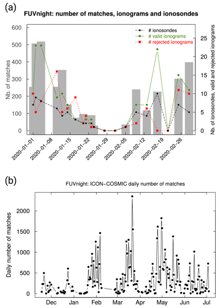
(a) Daily number of matches (gray shade) between FUV and ionosonde profiles. The green and red lines show the daily number of valid and rejected ionograms, while the black line represents the daily number of distinct ionosonde stations (right axis). (b) Daily number of matches between FUV and C2.

3.1. Conjugate Photoelectron Impact

The (a) and (c) panels of Figure 3 correspond to scatter plots of ICON and C2/ionosonde N_mF₂ values, binned in hexagonal cells so that counts are reported, instead of single values, which has the advantage to highlight the plot region where the point density is the largest (light blue)

Figure 3.

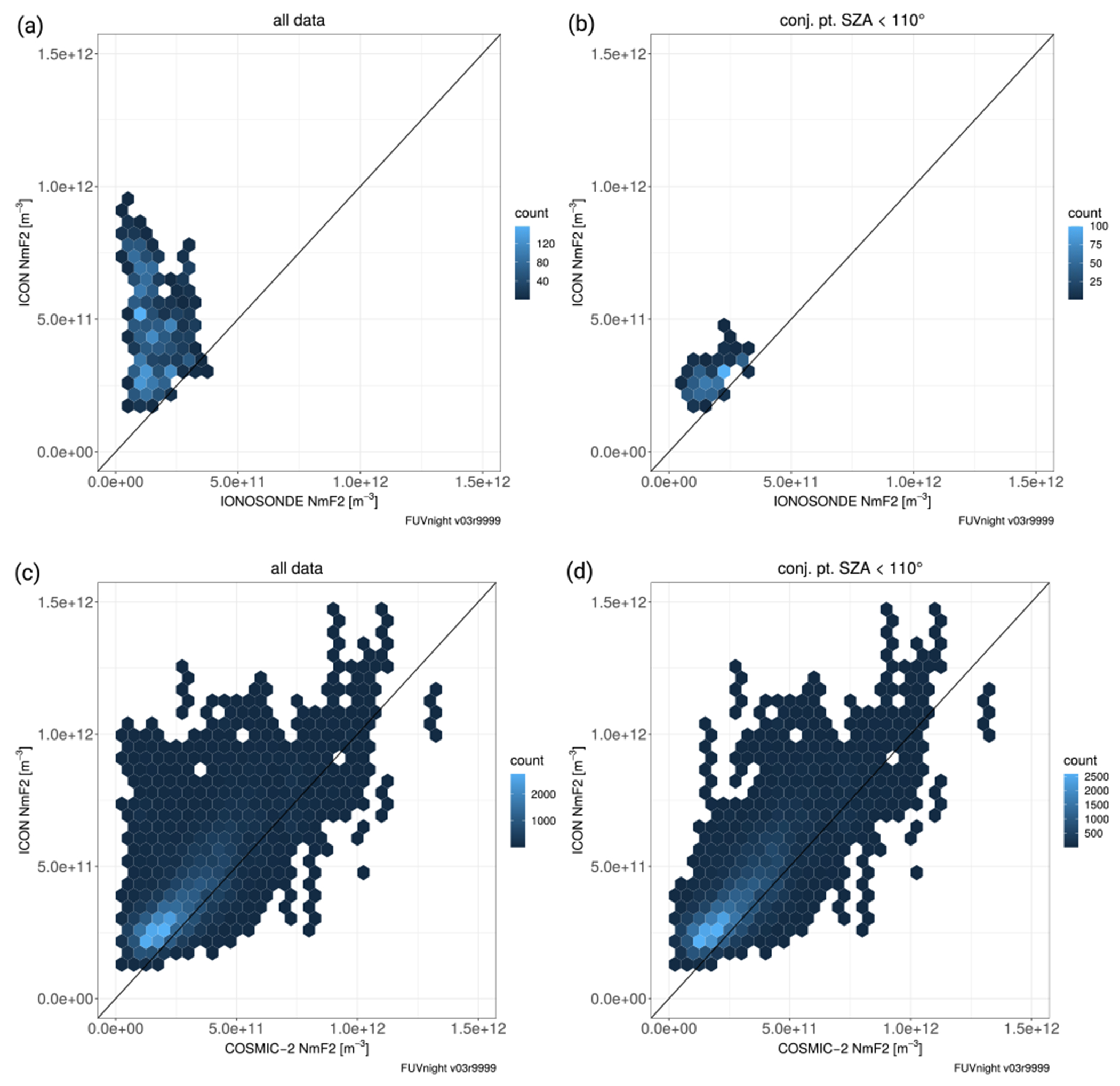
Scatter plots of N_mF₂ before (a) and (c) and after (b) and (d) filtering of conjugate photoelectrons for ionosonde (a) and (b) and C2 (c) and (d) comparisons.

They show that on average the FUV measurements show a larger N_mF₂ value than C2 and ionosondes. This is particularly true for ionosonde comparison where data are not distributed around the y = x bisector line. The largest disagreement between FUV and ionosondes is found to be correlated to an FUV brightness excess which can be caused by photoelectrons originating from areas of the conjugate hemisphere which are still illuminated. These electrons are transported along the magnetic field lines and precipitate into the nighttime atmosphere, where they excite atoms and molecules which, in turn, emit in the ultraviolet OI–135.6 nm line, among others. This mechanism has been known for years (Meier, 1971) and recent studies observed its effect from Defense Meteorological Satellite Program (DMSP) spacecraft and Global-scale Observations of the Limb and Disk (GOLD) observatory (Kil et al., 2020; Solomon et al., 2020). To avoid contamination of FUV data by this physical mechanism, we also exclude data for which the SZA at the conjugate point is smaller than 110°, which ensures that the latter is located in darkness, from the Earth’s surface up to about 400 km altitude. The updated scatter plots that discard conjugate photoelectrons are displayed in panels (b) and (d) of Figure 3. With respect to (a) and (b) panels, the updated data set shows a dramatic change of the distribution in the case of the ionosonde comparison while only some data points disappear for C2 case. This is due to the fact that the ionosonde data set period spans over January and February only, against several months for C2 (see above). Indeed, because the angle between the solar terminator and a meridian is larger around solstices, the conditions for which FUV conjugate points are illuminated are clustered during the winter months. Let us specify that the angle between the solar terminator and magnetic meridian is declination-dependent, and so the contribution of conjugate photoelectrons. In this study, all ionosondes are located in geographic areas where magnetic declination is low (around 10°), meaning that magnetic and geographic meridians are approximately parallel so that solstices mostly correspond to the epoch of the year when the angle between the terminator and the meridian is the largest. In a more general way, it is important to compute the angle between the magnetic meridian and the terminator to better assess the importance of photoelectron contribution. We note that conjugate photoelectron filtering significantly reduces the size of the ionosonde data set, with a total number of matches decreasing from 3278 to 563. On the other hand, the C2 data set only sees its size dropping from 63,684 to 59,997.

3.2. COSMIC-2 Difference Maps

Because of the mostly uniform distribution of FUV-C2 matches at the global scale, it is straightforward to map the differences using a binning technique to represent the information on a regular grid. This technique cannot be applied to the ionosonde data set because of the fixed location of the facilities. Figure 4 shows maps of N_mF₂ and h_mF₂ differences, further referred to as ΔN_mF₂ and Δh_mF₂.

Figure 4.

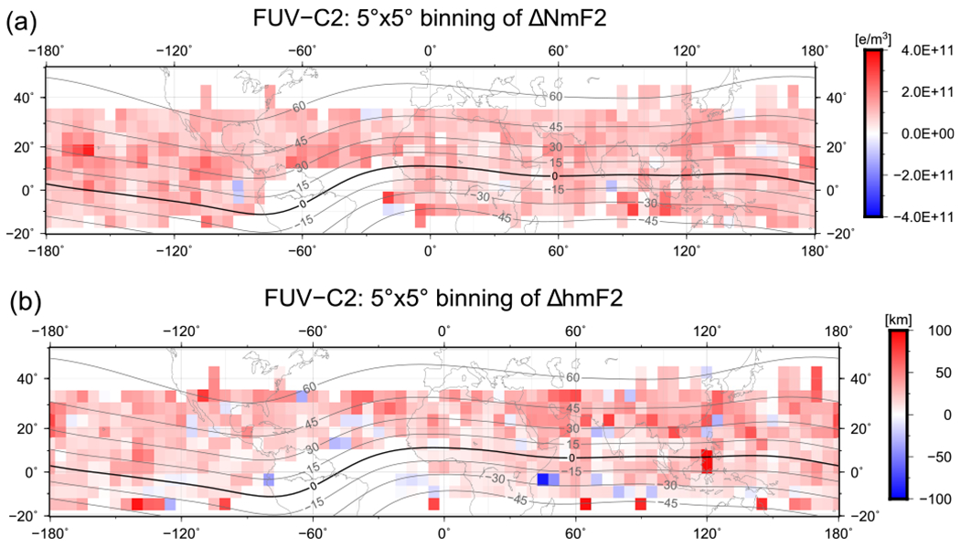
5° × 5° bins of averaged ΔN_mF₂ (a) and Δh_mF₂ (b) for FUV-C2 comparison. Contour lines correspond to geomagnetic inclination. Note the data gap around the South Atlantic Anomaly (SAA) over South America which results from shutting down the instrument to protect it from energetic particles.

The aggregating function used for the 5° × 5° binning is the average. The analysis of Figure 4 indicates that FUV N_mF₂ and h_mF₂ values are generally larger than the C2 ones (positive difference). N_mF₂ differences seem to be uniformly distributed on the map, while h_mF₂ differences are larger at midlatitudes in the northern hemisphere. On the contrary, there is no observational evidence of any longitudinal dependence of the differences, despite the existence of some clusters (e.g., Caribbean, Hawaii, and East Pacific sectors).

3.3. Summary Statistics

Figure 5 shows the histograms of ΔN_mF₂ and Δh_mF₂ between FUV and radio-sounding data sets. In addition, mean and standard deviation in both absolute and relative values are available in Table 1. It is also important to mention the absolute values of N_mF₂ and h_mF₂ which are related to the differences analyzed in this work. The density mean values of 4.1 × 10¹¹ (±2 × 10¹¹) [m⁻³] , 3 × 10¹¹ (±1.8 × 10¹¹) [m⁻³] and 1.7 × 10¹¹ (±0.6 × 10¹¹) [m⁻³] for FUV, C2, and ionosonde data sets, respectively, are typical of very low solar conditions encountered during the analysis period. Peak height mean values are normally distributed around 302 (±33) km, 287 (±37) km, and 270 (±21) km for FUV, C2, and ionosonde data sets, respectively.

Figure 5.

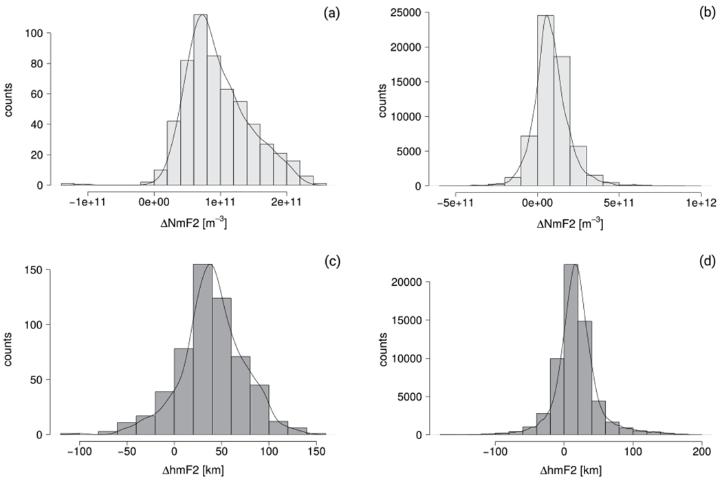
Histograms and their related kernel density estimation of ΔN_mF₂ between FUV and ionosondes (a), ΔN_mF₂ between FUV and C2 (b), and the estimation of Δh_mF₂ between FUV and ionosondes (c) and the estimation of Δh_mF₂ between FUV and C2 (d).

Table 1.

Mean and Standard Deviation of Ionospheric Parameter Differences Between FUV and Ionosonde and C2 Data

	N	ΔNmF2[m−3]	ΔNmF2 [%]	ΔhmF2 [km]
FUV-COSMIC-2	59,997	9.6 × 1010	55	15
		±1.1 × 1011	±104	±31
FUV-ionosonde	563	9.6 × 1010	72	38
		±5.1 × 1010	±60	±35

On average, ΔN_mF₂ is approximately equal to 9.6 × 10¹⁰e/m³ for both comparison data sets with FUV, meaning that the ionosonde and C2 peak densities are consistent with each other during nighttime. The standard deviation of ΔN_mF₂ is smaller for the ionosonde data set than for C2, probably because manually scaled ionosonde profiles are more precise and accurate. The preliminary C2 cal/val report for space-weather data (Straus et al., 2020) points out that the difference in ionospheric critical frequency f_oF₂ between ionosondes and C2 at midlatitudes is lower than 0.5 MHz, which represents an electron density difference of 6.2 × 10¹⁰ e/m³ for a typical nighttime f_oF₂ value of 5 MHz. This difference is compatible with our results, even if the mean statistics seem to indicate that ionosonde and C2 very strongly agree on the average.

The relatively large difference values of about 55% and 72% for C2 and ionosonde data sets respectively can be due to the very small density values that were observed during the first months of the ICON mission, that is, during the current, historically deep solar minimum. Indeed, a very dim airglow leading to a very faint signal in the FUV detector would severely impact relative values. This effect is expected to be mitigated when larger N_mF₂ values will occur, as a consequence of the increase of the solar activity. This can be demonstrated in Figure 6a representing the average FUV-C2 ΔN_mF₂ (ordinate axis) for all conjunctions having a C2 N_mF₂ value larger than a given threshold (abscissa axis). Similar plots can be produced based on the ionosonde data set and lead to similar conclusions.

Figure 6.

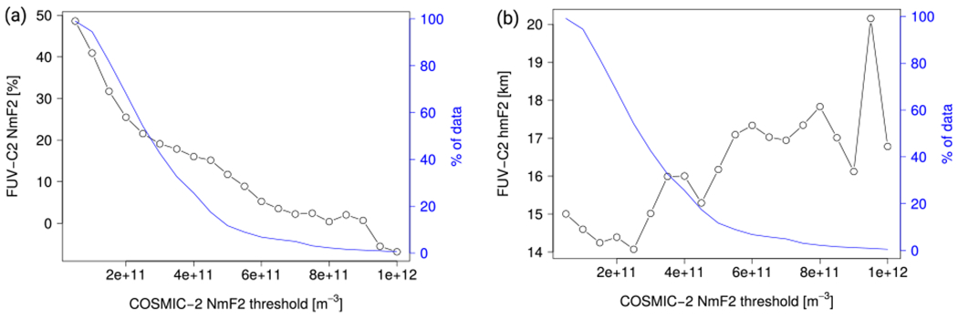
Relative ΔN_mF₂ (a) and absolute Δh_mF₂ values (b) with respect to C2. The x-axis represents the C2 N_mF₂ threshold used to compute the mean relative difference, that is, all measurements for which N_mF₂ is larger than this given threshold are participating to the average plotted on the y-axis. The right axis represent the fraction of the measurements participating to each data point.

Figure 6a shows that, as the density threshold increases, the relative difference drops from about 50% to negative values ranging between −10% and −20%. We can also observe that the number of observations participating to the data points (right axis) drops with increasing threshold, as most of the conjunctions are related to weak to moderate N_mF₂ values under the low solar activity conditions prevailing here. For density values ranging between about 5 × 10¹¹ and 1 × 10¹², we can observe that the mean difference in N_mF₂ lies within ±10%. This means that, if we are considering observations in a given signal range corresponding to an N_mF₂ background of at least 5 × 10¹¹e/m³, the FUV performance during nighttime allows for reliable electron density measurement. It comes that reliable O⁺ density measurement performances can be expected when the nighttime electron and ion densities are larger than those of a deep, prolonged solar minimum.

Turning to h_mF₂, Figure 5 and Table 1 indicate that FUV provides larger values than ionosondes and C2, with a mean difference of about 15 km for C2 and 38 km for ionosondes. Note that the 23 km difference between the two radio-sounding comparison data sets is significant, and roughly corresponds to one half of the ionospheric scale height at the peak altitude under low solar activity conditions. Both the FUV-C2 and FUV-ionosonde comparisons therefore lead to Δh_mF₂ average values representing a substantial fraction of the scale height. The influence of the FUV sensitivity on h_mF₂ can also be discussed based on Figure 6b. The h_mF₂ value is not very sensitive to the absolute N_mF₂ value, despite a clear slight increase with increasing N_mF₂ values. The ionospheric peak height difference with respect to radio-sounding data sets remains therefore independent on the background conditions, meaning that sensitivity is not a limiting factor for this variable.

In addition, we investigated the Solar Local Time (SLT) and SZA dependence on both N_mF₂ and h_mF₂ differences. The complete analysis and related figure can be found in Figure S1 in Supporting Information S1. We found that SZA and SLT results are consistent with each other but C2 and ionosonde data sets lead to different conclusions. No statistical significant information can be extracted from both C2 and ionosonde data set analysis, but differences between the pre-dawn and post-dusk conditions are suggested.

4. Discussion and Future Work

In the methodology section, it has been chosen to set the maximum matching distance (ΔD) to 500 km. In Figure 7, we investigate how sensitive to this threshold are the mean and standard deviation values summarized in Table 1. Because the data set sample size is much larger for C2 than for the ionosondes, the following analysis relies on this single data set to ensure a sufficient statistical power to the results. It comes from Figure 7a that both mean and standard deviation values of ΔN_mF₂ slightly decrease with decreasing ΔD. These results are compatible with the natural spatial autocorrelation of the ionosphere: the closer the profile locations, the closer their related attribute. However, ΔN_mF₂ does not asymptotically decrease to zero with decreasing ΔD. There remains a positive difference, or bias, of 9.2 × 10¹⁰ e/m³ between the two data sets, FUV data providing larger N_mF₂ values than C2. The drop of the standard deviation values with decreasing ΔD was also expected and means that, on the average, profiles are closer to each other when the distance between their respective tangent points is smaller. On the contrary, the differences in h_mF₂ do not decrease as a function of decreasing ΔD: Figure 7b shows a slight increase of about 1.5 km between the original statistics (using a 500 km threshold) and ΔD = 50 km. The standard deviation also drops by 4 km for the smallest ΔD value, indicating that the mean Δh_mF₂ value is more precise, without a surprise. A similar study has been conducted to assess the influence of the time difference (ΔT), fixed at 15 min. We found that observations closer to each other from the ΔT point of view do not lead to a decrease of the mean and of the standard deviation of the differences. Indeed, taking observations closer in terms of time difference involve considering observations that are more distant from each other, which does not make the differences decrease. The spatial distance seems therefore to be the matching parameter that mostly influences the differences.

Figure 7.

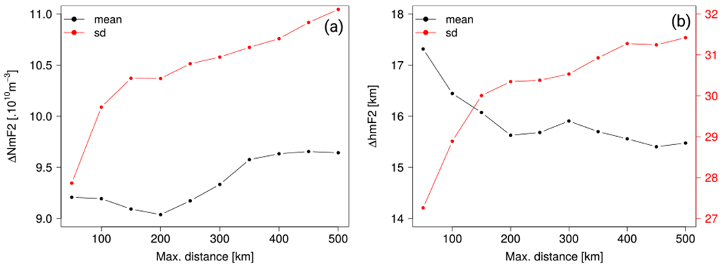
Influence of maximum matching distance on mean and standard deviation of ΔN_mF₂ (a) and Δh_mF₂ values (b).

As explained in the methodology section, the IRI model is also run for each conjunction. The difference between IRI runs at ICON location and observation time and at C2 (or ionosonde) location and observation time is therefore computed for each match, allowing us to assess the expected climatological difference between the two measurements. It comes that the mean and standard deviation of IRI-to-IRI comparisons are 0.8% (±15.6%) for the FUV-C2 data set and −2.1% (±6.9%) for the FUV-ionosonde data set. It comes that these mean differences are negligible compared to the observed differences discussed in the results section. However, the standard deviation values are here not negligible and future investigations may consider mitigating the climatological trends by removing the IRI-to-IRI differences to obtain even more precise statistics. These conclusions do not impact the work and results presented here, as the climatological differences are one order of magnitude smaller than the observed differences.

Concerning the comparisons between optical (FUV) and radio (C2) measurements, a perfect match is not expected as the physical phenomenon observed in both techniques is different. While the atmosphere is completely transparent to radio waves, the airglow emission is partially absorbed by molecular oxygen. This is particularly true for low tangent point altitudes. As a result, even for a perfectly spherical symmetric ionosphere and assuming an identical line of sight, the integrated quantities are not expected to exactly correspond to the same segment of the ionosphere. However, the way the retrieval algorithms take into account the plasma inhomogeneity and the partial absorption of airglow radiations is beyond the scope of this article but should be considered in future investigations.

The results of Section 3 aggregate the whole ICON data availability period but do not consider potential changes of the differences with time. Because of ICON and C2 orbit precession and of the change of solar illumination conditions throughout the year, we can not exclude the presence of unexpected trends with time of the mean statistics described in the previous section. Figure 8 shows time series of daily mean value of ΔN_mF₂ and Δh_mF₂, together with the daily mean geographic latitude of the tangent points. The first striking observation is the presence of obvious cycles in the mean conjunction latitude (Figure 8c). This means that, at a given observation period, the statistics mainly concern a particular latitude band. Because we previously demonstrated that latitude considerably impacts the summary statistics, it is expected that the daily mean ΔN_mF₂ and Δh_mF₂ follow the latitude pattern. ΔN_mF₂ is sometimes in phase (mid-December), sometimes in anti-phase (mid-January) with the mean latitude of the conjunctions (Figure 8a). The ΔN_mF₂ variability is lower from mid-April and onwards, with damped or even nonexistent cycles. This probably stems from the introduction of the dynamic background subtraction algorithm, set up from beginning of April, that better characterizes and subtracts the background emission in the 135.6 nm channel. The h_mF₂ differences of Figure 8b do not seem to be correlated with the location of the C2 conjunctions and are uniformly distributed around the mean value. No trend is visible in both the FUV density and height time series, meaning that summary statistics do correctly represent the mean behavior of the instrument.

Figure 8.

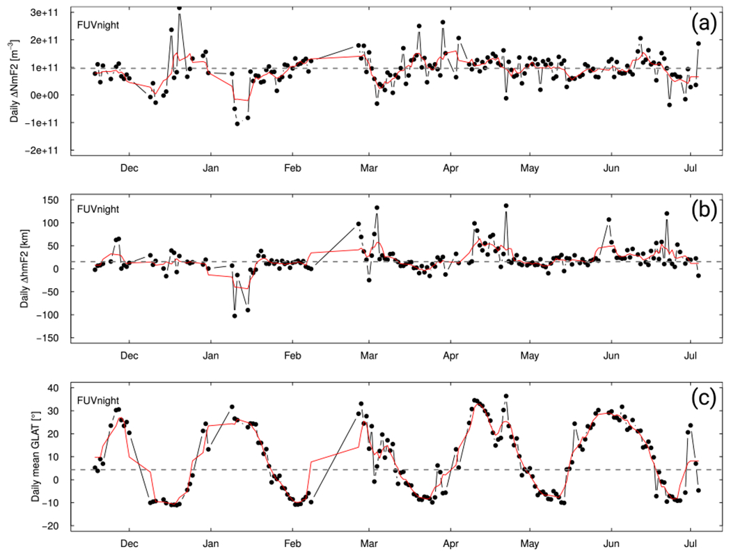
C2 comparison. Time series of FUV daily mean ΔN_mF₂, Δh_mF₂ and geographic latitude. The corresponding 5-day running mean is plotted with the solid red line. The mean values for the whole data sets are plotted with the dashed gray line and correspond to the values appearing in Table 1.

Another comparison source of interest are the Incoherent Scatter Radars (ISR) which provide the most accurate measurement of N_mF₂ and h_mF₂. An N_mF₂ comparison has been carried between the ISR of Millstone Hill and the ionosonde located in the vicinity of the ISR facility. As for the previous analyses, ionogram sequences have been manually scaled and validated. Two punctual comparison tests have been performed: the first, between 2020-01-29 and 2020-02-07, during nighttime hours and the second during daytime, from 2020-11-04 to 2020-11-13. Millstone Hill ISR provides observations at a sampling rate of several minutes, which is compatible with that of the ionosonde. For the two comparisons, the maximum time difference between ISR and ionosonde data is less than 3 min, meaning that observations can be considered as nearly simultaneous, in addition to be perfectly co-located. N_mF₂ mean differences are 1.2% (±3.3%) for nighttime hours and −3.1% (±3.3%) during daytime. These small differences demonstrate how accurate are the ionosonde measurements after manual scaling, which gives very high confidence in the statistics presented in Section 3. In the future, the FUV profile comparison with ISR, if possible for all latitude bands, would be a valuable way of characterizing the confidence to have in ICON ionospheric peak density and height measurements.

Another way of assessing the accuracy and the consistency between radio-sounding methods is to look for conjunctions between C2 and ionosondes. The existing literature already assessed in numerous studies the first COSMIC mission overall performance and the general conclusions converge toward a very good agreement between the two data sources. For instance, Lei et al. (2007), computed a correlation coefficient value of 0.85 in July 2006 between COSMIC and ionosonde N_mF₂. Cherniak and Zakharenkova (2014), based on comparison of COSMIC and the mid-latitude ISR of Kharkov (Ukraine) found that the correlation was larger when the radio occultation trace is oriented east-west rather than north-south, due to the fact that meridional gradients are generally larger than zonal ones. In addition, the authors observed a 2% mean N_mF₂ difference between ISR and COSMIC and 8 km in h_mF₂. Other studies computed correlation coefficient of 0.98 and 0.95 for N_mF₂ and h_mF₂, respectively, over the European region (Krankowski et al., 2011). Mean differences are less than 2% for both parameters, with standard deviation values being about 8% for N_mF₂ and 11 km for h_mF₂. Simulations at low-latitude point out an expected lower performance of radio occultation retrieval algorithms when the ionization crests are crossed by the line of sight (Yue et al., 2010). At the present time, very few studies characterize (e.g., Lin et al., 2020) the overall performance of the second generation of COSMIC constellation, namely COSMIC-2. Remember that COSMIC-2 electron density profiles are retrieved using the so-called Ne-aided Abel inversion method, which takes into account the three-dimensional heterogeneity of the electron density plasma (Chou et al., 2017), so that C2 is expected to provide more precise and accurate electron density profiles than the former COSMIC mission. Very recently, Cherniak et al. (2021) assessed the accuracy of C2 peak parameters under quiet geomagnetic conditions using manually scaled ionograms. The mean h_mF₂ difference is 5 and 2 km at low and middle latitudes, respectively. Concerning peak density, the authors show that the mean and RMS f_oF₂ difference is about 0.5 MHz, with corresponding relative values of 6%–9% from the reference ionosonde values. In this study, some conjunctions have the particularity to be a triple conjunction, that is, a special match where ICON, C2, and ionosonde provide simultaneous and synchronized observations. As a preliminary study, we analyze four triple conjunctions occurring in September 2020. They show that, on the average, C2 N_mF₂ values were 29% larger than those of ionosondes, which is significantly different from zero. Therefore, observed N_mF₂ differences do not seem to agree well with the existing literature related to the radio-occultation method and with the f_oF₂ RMS of about 0.5 MHz (Cherniak et al., 2021; Straus et al., 2020), which corresponds to much smaller differences than the observed 30%. On the contrary?, the h_mF₂ differences are about 6 km on the average, the lower values being always observed with ionosondes. This is compatible with the intrinsic altitude error measurement and with the results of Cherniak et al. (2021), in addition to the C2 and ionosonde altitude resolution of several km. In conclusion, C2 and ionosonde agree on peak height but significantly disagree on the density value for the small number of triple conjunctions analyzed in the framework of this study. Because such N_mF₂ differences, which can influence the final results of our comparison study, slightly disagree with the literature, future investigations should be carried on this topic. However, the final agreement between C2 and ionosondes is expected to be better as soon as final C2 space weather “ionPrf” product is available. Indeed, the C2 profiles considered in this study are related to the current “provisional” C2 data, which were the only space weather data available at the time this study was written.

The common point between ICON and C2 observations is the line of sight integration of a quantity, which is then inverted to get the O⁺ or electron density profiles. The comparison between two profiles coming from these two techniques should be, in principle, smaller when the two lines of sight are similar and cross the same ionospheric regions and gradients. Therefore, it is worth looking at similar line of sight azimuths to expect reducing the differences between ICON and C2. Selecting an azimuth difference of maximum 30° reduces drastically the sample size for which summary statistics similar to Table 1 have been computed. Despite a very slight absolute decrease in ΔN_mF₂, the other summary statistics remain very close to the values found without azimuth filtering. Then, contrary to our expectations, such geometry filtering does not improve significantly the precision and accuracy of our comparison study.

In this last paragraph, we attempt to find physical explanations for the differences that have been observed in Section 3 and discussed above. FUV density differences with respect to C2 and ionosondes are similar and consist of slighter larger values. In an airglow measurement, the existence of a density enhancement is inferred based on an excess in brightness measurement that could be due to several factors. We note that the bias represents about 50% of the smallest N_mF₂ values but can drop down to 10% if larger N_mF₂ values are observed. Let us also remind that the mutual neutralization, which is a loss mechanism for O⁺ ions, is already taken into account in the inversion algorithm (Kamalabadi et al., 2018) and cannot therefore explain the density differences. We also exclude the effect of particle precipitation occurring in regions that ICON cannot observe and that of conjugate photoelectrons that have been excluded from our data set (see Section 3.1). A constant bias may be related to an offset in the background characterization when raw counts are converted into brightness units, that is, Rayleigh. However, the dynamical background subtraction has already shown its efficiency by mitigating the variability in the N_mF₂ differences, as shown in Figure 8. It is also worth mentioning that several background subtraction algorithms have been tested and validated by the FUV team. Their comparison shows very little differences in the O⁺ density profiles, so that the choice of the algorithm does not significantly impact the results observed for N_mF₂ and h_mF₂ differences. Another source of brightness excess may be the presence of stars in the field of view. These stars are however filtered out by an appropriate algorithm based on a smoothing of the observations, which would have the opposite result, namely a lowering of N_mF₂ values. In future work, one should investigate the radiative transfer of the 135.6 nm emission, and particularly focus on scattering light that can produce additional scene illumination. The origin of light scattering can be off-axis solar or lunar radiation, reflected or partially transmitted into the optical parts of the instrument.

5. Conclusion

We present the first comparison of ICON-FUV O⁺ density profiles with ground and space-based measurements performed by ionosondes and the COSMIC-2 mission. The analysis period ranges from November 2019 to July 2020. Because of the need of ionogram manual validation and scaling, the size of the related data set is much smaller than that of C2 and only concerns January and February 2020. The impact of photoelectrons coming from the magnetically conjugate points can be easily detected with FUV, which opens perspectives for a detailed study of this phenomenon. FUV nighttime profiles provide generally larger N_mF₂ values than radio-sounding methods, which are characterized by a bias of less than 1 × 10¹¹ e/m³ whose relative importance decreases with increasing N_mF₂ value. The impact of this bias is however background dependent: the larger the N_mF₂ value, the smaller will be the contribution of the positive bias observed. Peak height differences are less than 20 km for C2 and around 38 km with respect to ionosondes, meaning that FUV data are more consistent with C2 than with ionosonde from the h_mF₂ point of view. Ingesting ICON-FUV density profiles into assimilative models or using them in the frame of comparative studies can therefore be performed considering the above-mentioned limitations and differences with respect to radio-sounding methods.

Key Points:

• We compare ICON-FUV NmF2 and hmF2 observations with those provided by COSMIC-2 and ionosondes

• Far Ultra Violet Imaging Spectrograph (FUV) observations are affected by conjugate photoelectrons mainly around solstices

• The FUV performance during nighttime allows for reliable electron density measurement

Data Availability Statement

ICON data are publicly available on ICON website, managed by the Space Sciences Laboratory, UC Berkeley, CA: https://icon.ssl.berkeley.edu/Data. Ionosonde data are available on the NOAA FTP archive: ftp.ngdc.noaa.gov/ionosonde/data/. COSMIC-2 “ionPrf” products are available at UCAR: https://doi.org/10.5065/t353-c093. Millstone Hill Incoherent Scatter Radar data are found on the Madrigal database of Millstone Hill: http://millstonehill.haystack.mit.edu/.

References

- Bilitza D, Altadill D, Truhlik V, Shubin V, Galkin I, Reinisch B, & Huang X (2017). International reference ionosphere 2016: From ionospheric climate to real-time weather predictions. Space Weather, 15(2), 418–429. 10.1002/2016SW001593 [DOI] [Google Scholar]
- Bust G, & Immel T (2020). IDA4D: Ionospheric data assimilation for the ICON mission. Space Science Reviews, 216. 10.1007/s11214-020-00648-z [DOI] [Google Scholar]
- Cherniak I, & Zakharenkova I (2014). Validation of FORMOSAT-3/COSMIC radio occultation electron density profiles by incoherent scatter radar data. Advances in Space Research, 53(9), 1304–1312. 10.1016/j.asr.2014.02.010 [DOI] [Google Scholar]
- Cherniak I, Zakharenkova I, Braun J, Wu Q, Pedatella N, Schreiner W, et al. (2021). Accuracy assessment of the quiet-time ionospheric F2 peak parameters as derived from COSMIC-2 multi-GNSS radio occultation measurements. Journal of Space Weather and Space Climate, 11, 18. 10.1051/swsc/2020080 [DOI] [Google Scholar]
- Chou MY, Lin CCH, Tsai HF, & Lin CY (2017). Ionospheric electron density inversion for global navigation satellite systems radio occultation using aided Abel inversions. Journal of Geophysical Research: Space Physics, 122(1), 1386–1399. 10.1002/2016JA023027 [DOI] [Google Scholar]
- Englert CR, Harlander JM, Brown CM, Marr KD, Miller IJ, Stump JE, et al. (2017). Michelson Interferometer for Global High-Resolution Thermospheric Imaging (MIGHTI): Instrument design and calibration. Space Science Reviews, 212(1), 553–584. 10.1007/s11214-017-0358-4 [DOI] [PMC free article] [PubMed] [Google Scholar]
- Harding BJ, Makela JJ, Englert CR, Marr KD, Harlander JM, England SL, & Immel TJ (2017). The MIGHTI wind retrieval algorithm: Description and verification. Space Science Reviews, 212(1), 585–600. 10.1007/s11214-017-0359-3 [DOI] [PMC free article] [PubMed] [Google Scholar]
- Heelis RA, Stoneback RA, Perdue MD, Depew MD, Morgan WA, Mankey MW, et al. (2017). Ion velocity measurements for the ionospheric connections explorer. Space Science Reviews, 212(1), 615–629. 10.1007/s11214-017-0383-3 [DOI] [PMC free article] [PubMed] [Google Scholar]
- Kamalabadi F, Qin J, Harding BJ, Iliou D, Makela JJ, Meier RR, et al. (2018). Inferring nighttime ionospheric parameters with the far ultraviolet imager onboard the ionospheric connection explorer. Space Science Reviews, 214(4), 70. 10.1007/s11214-018-0502-9 [DOI] [PMC free article] [PubMed] [Google Scholar]
- Kil H, Schaefer RK, Paxton LJ, & Jee G (2020). The far ultraviolet signatures of conjugate photoelectrons seen by the special sensor ultraviolet spectrographic imager. Geophysical Research Letters, 47(1), e2019GL086383. 10.1029/2019GL086383 [DOI] [Google Scholar]
- Krankowski A, Zakharenkova I, Krypiak-Gregorczyk A, Shagimuratov I, & Wielgosz P (2011). Ionospheric electron density observed by FORMOSAT-3/COSMIC over the European region and validated by ionosonde data. Journal of Geodesy, 85, 949–964. 10.1007/s00190-011-0481-z [DOI] [Google Scholar]
- Lei J, Syndergaard S, Burns AG, Solomon SC, Wang W, Zeng Z, et al. (2007). Comparison of COSMIC ionospheric measurements with ground-based observations and model predictions: Preliminary results. Journal of Geophysical Research, 112(A7). 10.1029/2006JA012240 [DOI] [Google Scholar]
- Lin C-Y, Lin CC-H, Liu J-Y, Rajesh PK, Matsuo T, Chou M-Y, et al. (2020). The early results and validation of FORMOSAT-7/COSMIC-2 space weather products: Global ionospheric specification and Ne-aided Abel electron density profile. Journal of Geophysical Research: Space Physics, 125(10), e2020JA028028. 10.1029/2020JA028028 [DOI] [Google Scholar]
- Meier RR (1971). Observations of conjugate excitation of the OI 1304-A airglow. Journal of Geophysical Research, 76(1), 242–247. 10.1029/ja076i001p00242 [DOI] [Google Scholar]
- Mende SB, Frey HU, Rider K, Chou C, Harris SE, Siegmund OHW, et al. (2017). The far ultra-violet imager on the ICON mission. Space Science Reviews, 212(1), 655–696. 10.1007/s11214-017-0386-0 [DOI] [PMC free article] [PubMed] [Google Scholar]
- Piggot W, & Rawer K (1978). U.R.S.I. handbook of ionogram interpretation and reduction, Revision of chapters 1-4 (Tech. Rep. No. UAG-23A). World data center A for Solar-Terrestrial Physics. (Revison Adopted by U.R.S.I. Commission III). [Google Scholar]
- Qin J, Makela JJ, Kamalabadi F, & Meier RR (2015). Radiative transfer modeling of the OI 135.6 nm emission in the nighttime ionosphere. Journal of Geophysical Research: Space Physics, 120(11), 10116–10135. 10.1002/2015JA021687 [DOI] [Google Scholar]
- Sirk MM, Korpela EJ, Ishikawa Y, Edelstein J, Wishnow EH, Smith C, et al. (2017). Design and performance of the ICON EUV spectrograph. Space Science Reviews, 212(1), 631–643. 10.1007/s11214-017-0384-2 [DOI] [PMC free article] [PubMed] [Google Scholar]
- Solomon SC, Andersson L, Burns AG, Eastes RW, Martinis C, McClintock WE, & Richmond AD (2020). Global-scale observations and modeling of far-ultraviolet airglow during twilight. Journal of Geophysical Research: Space Physics, 125(3), e2019JA027645. 10.1029/2019JA027645 [DOI] [Google Scholar]
- Stephan AW, Korpela EJ, Sirk MM, England SL, & Immel TJ (2017). Daytime ionosphere retrieval algorithm for the Ionospheric Connection Explorer (ICON). Space Science Reviews, 212(1), 645–654. 10.1007/s11214-017-0385-1 [DOI] [PMC free article] [PubMed] [Google Scholar]
- Stephan AW, Meier RR, England SL, Mende SB, Frey HU, & Immel TJ (2018). Daytime O/N2 retrieval algorithm for the Ionospheric Connection Explorer (ICON). Space Science Reviews, 214(1), 42. 10.1007/s11214-018-0477-6 [DOI] [PMC free article] [PubMed] [Google Scholar]
- Stevens MH, Englert CR, Harlander JM, England SL, Marr KD, Brown CM, & Immel TJ (2017). Retrieval of lower thermospheric temperatures from O2 A band emission: The MIGHTI experiment on ICON. Space Science Reviews, 214(1), 4. 10.1007/s11214-017-0434-9 [DOI] [PMC free article] [PubMed] [Google Scholar]
- Straus P, Schreiner W, Santiago J, Talaat E, & Lin C-L (2020). FORMOSAT-7/COSMIC-2 TGRS Space Weather Provisional Data Release 1. (Tech. Rep.). NOAA, USAF and NSPO. [Google Scholar]
- Thébault E, Finlay CC, Beggan CD, Alken P, Aubert J, Barrois O, et al. (2015). International geomagnetic reference field: The 12 th generation. Earth, Planets and Space, 67(1), 79. 10.1186/s40623-015-0228-9 [DOI] [Google Scholar]
- Yue X, Schreiner WS, Lei J, Sokolovskiy SV, Rocken C, Hunt DC, & Kuo Y-H (2010). Error analysis of Abel retrieved electron density profiles from radio occultation measurements. Annales Geophysicae, 28(1), 217–222. 10.5194/angeo-28-217-2010 [DOI] [Google Scholar]
- Yue X, Schreiner WS, Lin Y-C, Rocken C, Kuo Y-H, & Zhao B (2011). Data assimilation retrieval of electron density profiles from radio occultation measurements. Journal of Geophysical Research, 116(A3). 10.1029/2010JA015980 [DOI] [Google Scholar]
Associated Data
This section collects any data citations, data availability statements, or supplementary materials included in this article.
Supplementary Materials