Estimation of most effected cycles and busiest network route based on complexity function of graph in fuzzy environment

Abstract

Connectivity and strength has a major role in the field of network connecting with real world life. Complexity function is one of these parameter which has manifold number of applications in molecular chemistry and the theory of network. Firstly, this paper introduces the thought of complexity function of fuzzy graph with its properties. Second, based on the highest and lowest load on a network system, the boundaries of complexity function of different types of fuzzy graphs are established. Third, the behavior of complexity function in fuzzy cycle, fuzzy tree and complete fuzzy graph are discussed with their properties. Fourth, applications of these thoughts are bestowed to identify the most effected COVID-19 cycles between some communicated countries using the concept of complexity function of fuzzy graph. Also the selection of the busiest network stations and connected internet paths can be done using the same concept in a graphical wireless network system.

Introduction

Research background

Mathematics serves an essential and important requirement in many fields. One of the most significant role in the field of mathematics is being played by graph theory in various innovative methods, structural models in strategic decision making under different discipline, determination of shortest path, computer network modelling. If a structure is constructed by a large or huge number of parts which interact in a non-straight forward way under a voluntary loading scheme, then we can say that the structure is complex. Complexity function has an egregious role to measurement of complexity in many applications of crisp graph as well as fuzzy graph.

The initial work on molecular topological complexity was emerged on the utilization of information theory in the study of complexity of living system and was published in several leading paper in the journal “Bulletin Mathematical Biophysics" (the current of the journal is “Bulletin of Mathematical Biology"). The intuition behind this perception was reductionist: The complexity of the life course is mainly constructed by complexity of the component organic molecules. In 1956, Trucco (1956) formulated the complexity index in the automorphism group of molecules. Since the molecular topology was not sufficient, he used the graph theoretical elements in his work. Then Mowshowitz (1968) proposed the structural information related to the complexity of graphs. In 1975, Minoli (1975) first introduce the notion of the complexity function in molecular graph, where the vertices and edges represent the molecular atoms and their corresponding bounds respectively. The authors in Bertz (1987), Todeschini and Consonni (2000) tried to find qualified index which will account for the complexity in molecules, paths and this was set by Minoli. Also derive complexity indices from the representation of molecular graphs, independent on information theory. Dehmer et al. (2019) initiated the measure of the complexity in directed graphs.

In 1965, the revolution of Zadeh’s fuzzy set theory Zadeh (1965) deliver mathematics a global concept in which uncertainty can be measured. Due to presence of uncertainty in vertices and edges of graphs, Rosenfield (1975) in 1975 explained fuzzy graph theory. Also Yeh and Bang (1975) independently introduced the notion of fuzzy graphs and their many applications. Mordeson et al. (2018a, 2018b) established various properties of fuzzy relation, fuzzy graphs and applications. Mathew et al. (2018a, 2018b) explained several kind of fuzzy graphs and their saturation properties. Bhutani and Rosenfeld (2003a, 2003b) introduced end nodes and strong arcs of fuzzy graphs. Different types of arcs and operations of fuzzy graphs have been explained in Mathew and Sunitha (2009); Mordeson and Peng (1994). Nagoorgani and Hussain (2008) introduced total fuzzy domination and connected fuzzy domination on different types of fuzzy graphs. They also gave the notion of global and connected fuzzy domination number for some standards graphs. In Thirunavukarasu et al. (2016) Thirunavukarasu et al. introduced complex fuzzy graphs in which the membership values of vertices and edges are complex numbers. Many indices and their real applications of fuzzy graphs in human trafficking and illegal immigration are described in Binu et al. (2019, 2020). Concepts of cycle, trees and bridges in fuzzy graph have been explained in Mordeson and Nair (2000); Sunitha and Vijayakumar (1999). Degree of vertex and threshold graphs are established in Ghorai and Jacob (2019); Ghorai and Pal (2016). Certain types of index, nodes and their degree are examined in Poulik and Ghorai (2020a, 2020b, 2020c). Different types of degrees of bipolar fuzzy graphs are described in Borzooei and Rashmanlou (2016). Many concepts and operations of bipolar fuzzy graphs are examined in Dudek and Talebi (2016); Lakdashti et al. (2019). Rashmanlou et al. (2015, 2016) introduced different categorical properties and products of bipolar fuzzy graph. Talebi (2018) introduced Cayley fuzzy graphs. Talebi et al. (2020, 2021) defined different types of irregular intuitionistic fuzzy graphs and irregular single valued neutrosophic graphs. Poulik and Ghorai (2021) introduced Wiener index of bipolar fuzzy graph with application in journeys order. Application of interval-valued fuzzy graph in education system are described in Poulik et al. (2020).

Motivation

In crisp graph, the membership values of vertices and edges are either 0 or 1 which inform the presence of vertices and edges in the graph. But in a connected network field there always appeared some problems like natural disaster, mechanical disturbances, excessive users, etc. So in this type of network field, the signal becomes up-down i. e., the signal in the stations and its surrounding areas are uncertain. Then the fuzzy graph Rosenfield (1975) can be used to control the system. Since membership values of vertices and edges lie in the closed interval [0, 1], fuzzy graph gives an actual measure of the signal strength of the stations and nearer areas between stations. If the signal becomes slow, then we have to find out the total load on the system which depend on the strengths of all the path between every pair of network stations. To indicate most loaded network stations, the complexity function of various vertex deleted fuzzy subgraphs can be used. If the system can be divided into some cycles then it will be easy to find out the most defective cycles. This will help to repair the system. This is why we have to introduce the complexity function of fuzzy cycle and fuzzy trees.

Organization of the paper

This paper deals with complexity function of fuzzy graph, which provides the measure of the complexity of fuzzy graph and cover all the vertices and edges. Section 2 contains some basic definitions which have been used in the next sections. Section 3 establishes the notion of complexity function of fuzzy graph and fuzzy subgraph and their properties with examples. Section 4 develops various boundaries of complexity function of fuzzy graph, isomorphic properties and completeness with examples. Section 5 illustrates the properties of complexity function of fuzzy cycles, fuzzy trees and regular fuzzy graphs. Two applications of our research work are proposed in Sect. 6, the first one is to determine the communication cycles in which the chances of spread is most and the second one is to mention the strengthening paths in a wireless network system. This paper ending with some conclusions in Sect. 7.

Preliminaries

Here some basic concepts related to fuzzy graphs are given, which have been used in the next sections. Thus some definitions are given below. Most of the definitions are taken from Mordeson and Nair (2000), Sunitha and Vijayakumar (1999), Cary (2018), Gani and Ahamed (2003).

Definition 1

Let A be a set. A fuzzy graph $\zeta$ is a pair $(\mu ,\tau )$, where $\mu$ be a fuzzy subset of A and $\tau$ be a fuzzy subset of $A\times A$ such that $\tau (a_i{a}_j)\le min\{\mu (a_i),\mu (a_j)\}$. Here $\tau$ is called a fuzzy relation on $\mu$. The crisp graph of $\zeta =(\mu ,\tau )$ is denoted by ${\zeta }^{\ast }=({\mu }^{\ast },{\tau }^{\ast })$, such that ${\mu }^{\ast }=\{a_i\in A:\mu (a_i)>0\}$ and ${\tau }^{\ast }=\{a_i{a}_j\in A\times A:\tau (a_i{a}_j)>0\}$. An element $a_i\in {\mu }^{\ast }$ called a vertex and an element $a_i{a}_j\in {\tau }^{\ast }$ called an edge of $\zeta$.

• A fuzzy graph ${\zeta }^{\prime }=({\mu }^{\prime },{\tau }^{\prime })$ is said to be a partial fuzzy subgraph of $\zeta =(\mu ,\tau )$ if ${\mu }^{\prime }(a_i)\le \mu (a_i),\forall a_i\in {{\mu }^{\prime }}^{\ast }$ and ${\tau }^{\prime }(a_i{a}_j)\le \tau (a_i{a}_j),\forall a_i{a}_j\in {{\tau }^{\prime }}^{\ast }$. In this case ${\zeta }^{\prime }=({\mu }^{\prime },{\tau }^{\prime })$ is called a fuzzy subgraph of $\zeta$ if ${\mu }^{\prime }(a_i)=\mu (a_i),\forall a_i\in {{\mu }^{\prime }}^{\ast }$ and ${\tau }^{\prime }(a_i{a}_j)=\tau (a_i{a}_j),\forall a_i{a}_j\in {{\tau }^{\prime }}^{\ast }$.

• A sequence of distinct vertices $a_0,a_1,\dots ,a_d$ is called a path P of length d if $\tau (a_{i-1},a_i)>0,i=1,2,\dots ,d$. An edge on P is said to be weakest if membership value of the edge is the least of the membership values of all edges on P. The membership value of the weakest edges is called the strength of the path P.

• ${\zeta }^{x_1}=({\mu }^{x_1},{\tau }^{x_1})$ is called a $x_1$-cut fuzzy subgraph of $\zeta =(\mu ,\tau )$ if ${\zeta }^{x_1}$ is a partial fuzzy subgraph of $\zeta$, where ${\mu }^{x_1^{\ast }}=\{a_i;{\mu }^{x_1}(a_i)\ge x_1\}$ and ${\tau }^{x_1^{\ast }}=\{a_i{a}_j;{\tau }^{x_1}(a_i{a}_j)\ge x_1\}$, $0\le x_1\le 1$.

• Two fuzzy graphs $\zeta =(\mu ,\tau )$ and ${\zeta }^{\prime }=({\mu }^{\prime },{\tau }^{\prime })$ are isomorphic to each other if there exists a bijective mapping f from $\zeta$ to ${\zeta }^{\prime }$ such that $\mu (a_i)={\mu }^{\prime }(f(a_i)),\forall a_i\in {\mu }^{\ast }$ and $\tau (a_i{a}_j)={\tau }^{\prime }(f(a_i{a}_j)),\forall a_i{a}_j\in {\tau }^{\ast }$.

Definition 2

A connected fuzzy graph $\zeta =(\mu ,\tau )$ is said to be a fuzzy tree if $\zeta$ has a spanning fuzzy subgraph $F=({\mu }^{\prime },{\tau }^{\prime })$ which is a tree, such that for all $a_i{a}_j$ not in F, there exists a path between $a_i$ and $a_j$ in F whose strength is greater than $\tau (a_i{a}_j)$. In this case, F is called the unique maximum spanning tree of $\zeta$.

Here $\zeta$ is said to be complete if $\tau (a_i{a}_j)=min\{\mu (a_i),\mu (a_j),\forall a_i,a_j\in {\mu }^{\ast }\}$.

Definition 3

Let $\zeta =(\mu ,\tau )$ be a fuzzy graph.

• The size of a fuzzy graph $\zeta$ is $S=\sum _{i\ne j}\tau (a_i{a}_j)$.

• The degree of a vertex $a_i$ in $\zeta$ is $deg(a_i)=\sum _{a_i\ne a_j}\tau (a_i{a}_j)$ and $deg(a_i)+\mu (a_i)$ is called total degree of the vertex $a_i$.

• If degree of all the vertices of $\zeta$ are equal, then $\zeta$ is called a regular fuzzy graph. $\zeta$ is totally regular if the total degree of all the vertices of $\zeta$ are equal.

Definition 4

A fuzzy graph $\zeta$ is said to be perfectly regular if it is both regular and totally regular. For a perfectly regular fuzzy graph $\zeta$, $\mu$ must be a constant function i.e., membership values of each vertex are equal.

Complexity function of a fuzzy graph

The word “complexity" is derive from the Latin word “com" and “plectere". “com" means “together" and “plectere" means “to plait". Various topological functions and indices of molecular graph have an egregious role in facility location, communication, cryptology, internet routing, decision making, etc. All of these depend on the strength of each path between every pair of vertices in graph theory. But to maintain the system, total strength of each path with associated vertices is more important to avoid the internet traffic jam. Therefore derivation the complexity measure of the system is essential. Thus in this section the complexity function of fuzzy graph is introduced. The properties of complexity function in fuzzy subgraphs are explained with example.

Definition 5

Let $\zeta =(\mu ,\tau )$ be a fuzzy graph of the graph ${\zeta }^{\ast }=({\mu }^{\ast },{\tau }^{\ast })$ such that order of ${\mu }^{\ast }$ is $\mid {\mu }^{\ast }\mid =d$ and order of ${\tau }^{\ast }$ is $\mid {\tau }^{\ast }\mid =s$. The complexity function of $\zeta$ is denoted by $CF(\zeta )$ and is defined as

$$\begin{array}{c}\hfill CF(\zeta )=\frac{\mathit{ds}}{d+s}\sum _{\begin{array}{c}{a}_i,a_j\in {\mu }^{\ast }\\ i>j\end{array}}\mu (a_i)\mu (a_j)S{P}_{\mathit{ij}}\end{array}$$

where $S{P}_{\mathit{ij}}$ is the sum of the strengths of all paths between $a_i$ and $a_j$. $i>j$ means for a pair of vertices $a_i,a_j$ only $S{P}_{\mathit{ij}}$ will be taken but again $S{P}_{\mathit{ji}}$ is not consider.

Example 1

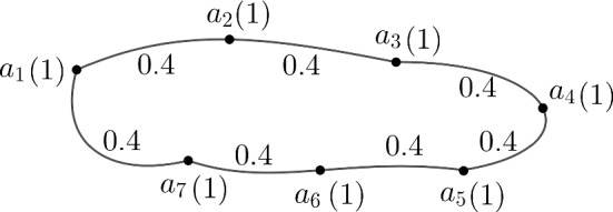
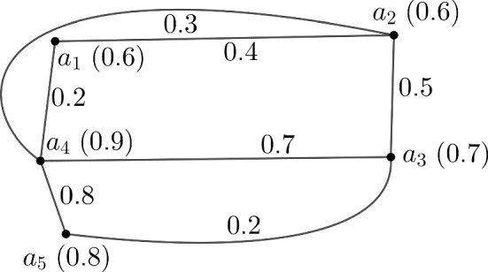
Consider a social network group of five friends $a_1,a_2,a_3,a_4,a_5$, shown in Fig. 1. Then ${\mu }^{\ast }=\{a_1,a_2,a_3,a_4,a_5\}$. A friend may active in the group between 0 hour to 24 hours. So, the activation time of each friend is uncertain. If a friend active 24 hours in a day then the membership value of the friend is 1 and if he/she can’t active then the membership value is 0. Suppose the $a_1$ active 9 hours 6 minutes in the group, then the membership value of $a_1$ is $\mu (a_1)=\frac{9.6}{24}=0.4$, Similarly, the membership values of the friends $a_2,a_3,a_4,a_5$ are $\mu (a_2)=0.3$, $\mu (a_3)=0.2$, $\mu (a_4)=0.5$, $\mu (a_5)=0.3$ respectively. Suppose the communication time between $a_1$ and $a_2$ is 2 hours 4 minutes. Then the membership value of the edge $a_1{a}_2$ is $\tau (a_1{a}_2)=\frac{2.4}{24}=0.1$. Similarly, the membership values of the edges $a_1{a}_3,a_1{a}_5,a_2{a}_3,a_3{a}_4,a_3{a}_5,a_4{a}_5$ are $\tau (a_1{a}_3)=0.2$, $\tau (a_1{a}_5)=0.2$, $\tau (a_2{a}_3)=0.1$, $\tau (a_3{a}_4)=0.2$, $\tau (a_3{a}_5)=0.1$, $\tau (a_4{a}_5)=0.2$ respectively. So, ${\tau }^{\ast }=\{a_1{a}_2,a_1{a}_3,a_1{a}_5,a_2{a}_3,a_3{a}_4,a_3{a}_5,a_4{a}_5\}$. Therefore, $\mid {\mu }^{\ast }\mid =d=5$ and $\mid {\tau }^{\ast }\mid =s=7$.

Fig. 1.

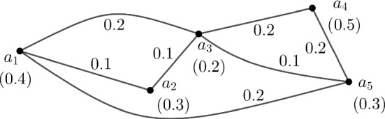
Representation of a social network group as a fuzzy graph $\zeta$

Now, $a_1-a_2$, $a_1-a_3-a_2$, $a_1-a_5-a_3-a_2$ and $a_1-a_5-a_4-a_3-a_2$ are the four paths between $a_1$ and $a_2$ with strengths 0.1, 0.1, 0.1, 0.1 respectively. So, $S{P}_{12}=0.1+0.1+0.1+0.1=0.4$, Similarly, $S{P}_{13}=0.6$, $S{P}_{14}=0.8$, $S{P}_{15}=0.7$, $S{P}_{23}=0.4$, $S{P}_{24}=0.6$, $S{P}_{25}=0.6$, $S{P}_{34}=0.6$, $S{P}_{35}=0.6$, $S{P}_{45}=0.6$.

$$\begin{array}{cc}\hfill CF(\zeta )=& \frac{5\times 7}{5+7}[0.048+0.048+0.16+0.084+0.024+0.09\hfill \\ \hfill & +0.054+0.06+0.036+0.09]=2.024.\hfill \end{array}$$

Theorem 1

Let ${\zeta }^{\prime }=({\mu }^{\prime },{\tau }^{\prime })$ be a partial fuzzy subgraph of the fuzzy graph $\zeta =(\mu ,\tau )$. Then $CF(\zeta )\ge CF({\zeta }^{\prime })$.

Proof

Let $\zeta =(\mu ,\tau )$ be a fuzzy graph with $\mid {\mu }^{\ast }\mid =d$, $\mid {\tau }^{\ast }\mid =s$ and ${\zeta }^{\prime }=({\mu }^{\prime },{\tau }^{\prime })$ be the partial fuzzy subgraph of $\zeta$ with $\mid {{\mu }^{\prime }}^{\ast }\mid =d^{\prime }$, $\mid {{\tau }^{\prime }}^{\ast }\mid =s^{\prime }$. Then ${{\zeta }^{\prime }}^{\ast }=({{\mu }^{\prime }}^{\ast },{{\tau }^{\prime }}^{\ast })$ must be a subgraph of the graph ${\zeta }^{\ast }=({\mu }^{\ast },{\tau }^{\ast })$. So, $d\ge d^{\prime }$, $s\ge s^{\prime }$ and hence

$$\begin{array}{c}\hfill \frac{\mathit{ds}}{d+s}\ge \frac{d^{\prime }{s}^{\prime }}{d^{\prime }+s^{\prime }}\dots \dots (I).\end{array}$$

Since the strength of any path lie on an edge in fuzzy graph, so the strength of a path in ${\zeta }^{\prime }$ must be less than or equal to the strength of that path in $\zeta$. Therefore, sum of the strengths of all paths between any two vertices $a_i$ and $a_j$ $(i.e.,S{P}_{\mathit{ij}}^{\prime })$ in ${\zeta }^{\prime }$ must be less than or equal to sum of the strengths of all paths between $a_i$ and $a_j$ $(i.e.,S{P}_{\mathit{ij}})$ in $\zeta$.

Thus, $S{P}_{\mathit{ij}}\ge S{P}_{\mathit{ij}}^{\prime }$, $\forall a_i,a_j\in {{\mu }^{\prime }}^{\ast }$

$$\begin{array}{cc}& \Rightarrow \mu (a_i)\mu (a_j)S{P}_{\mathit{ij}}\ge {\mu }^{\prime }(a_i){\mu }^{\prime }(a_j)S{P}_{\mathit{ij}}^{\prime },\forall a_i,a_j\in {{\mu }^{\prime }}^{\ast }\hfill \\ & \Rightarrow \sum _{\begin{array}{c}{a}_i,a_j\in {\mu }^{\ast }\\ i>j\end{array}}\mu (a_i)\mu (a_j)S{P}_{\mathit{ij}}\ge \sum _{\begin{array}{c}{a}_i,a_j\in {{\mu }^{\prime }}^{\ast }\\ i>j\end{array}}{\mu }^{\prime }(a_i){\mu }^{\prime }(a_j)S{P}_{\mathit{ij}}^{\prime }\dots \dots (II).\hfill \end{array}$$

Now, from (I) and (II), we have

$$\begin{array}{c}\hfill \frac{\mathit{ds}}{d+s}\sum _{\begin{array}{c}{a}_i,a_j\in {\mu }^{\ast }\\ i>j\end{array}}\mu (a_i)\mu (a_j)S{P}_{\mathit{ij}}\ge \frac{d^{\prime }{s}^{\prime }}{d^{\prime }+s^{\prime }}\sum _{\begin{array}{c}{a}_i,a_j\in {{\mu }^{\prime }}^{\ast }\\ i>j\end{array}}{\mu }^{\prime }(a_i){\mu }^{\prime }(a_j)S{P}_{\mathit{ij}}^{\prime }.\end{array}$$

Therefore $CF(\zeta )\ge CF({\zeta }^{\prime })$. $\square$

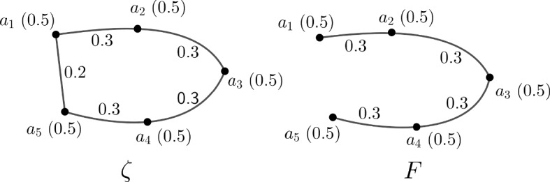
Example 2

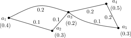
Consider the fuzzy graph ${\zeta }^{\prime }=({\mu }^{\prime },{\tau }^{\prime })$ of Fig. 2 with ${{\mu }^{\prime }}^{\ast }=\{a_1,a_2,a_3,a_4,a_5\}$. Here $a_1,a_2,a_3,a_4,a_5$ are communicated friends in a social network group like Example 1. ${{\tau }^{\prime }}^{\ast }=\{a_1{a}_2,a_1{a}_3,a_2{a}_3,a_3{a}_4,a_3{a}_5,a_4{a}_5\}$. Here $\mid {{\mu }^{\prime }}^{\ast }\mid =d^{\prime }=5$, $\mid {{\tau }^{\prime }}^{\ast }\mid =s^{\prime }=6$, ${\mu }^{\prime }(a_1)=0.4$, ${\mu }^{\prime }(a_2)=0.3$, ${\mu }^{\prime }(a_3)=0.2$, ${\mu }^{\prime }(a_4)=0.5$, ${\mu }^{\prime }(a_5)=0.3$ and ${\tau }^{\prime }(a_1{a}_2)=0.1$, ${\tau }^{\prime }(a_1{a}_3)=0.2$, ${\tau }^{\prime }(a_2{a}_3)=0.1$, ${\tau }^{\prime }(a_3{a}_4)=0.2$, ${\tau }^{\prime }(a_3{a}_5)=0.1$, ${\tau }^{\prime }(a_4{a}_5)=0.2$. Clearly ${\zeta }^{\prime }$ is partial fuzzy subgraph of the fuzzy graph $\zeta$ in Example 1.

Fig. 2.

A partial fuzzy subgraph ${\zeta }^{\prime }$ of the fuzzy graph $\zeta$ of Fig. 1

Now in ${\zeta }^{\prime }$, there are only two paths $a_1-a_2$ and $a_1-a_3-a_2$ between $a_1$ and $a_2$. Strengths of $a_1-a_2$ and $a_1-a_3-a_2$ are 0.1 and 0.1. Sum of the strengths of all the paths between $a_1$ and $a_2$ in ${\zeta }^{\prime }$ is $S{P}_{12}^{\prime }=0.2$. Similarly, $S{P}_{13}^{\prime }=0.3$, $S{P}_{14}^{\prime }=0.5$, $S{P}_{15}^{\prime }=0.5$, $S{P}_{23}^{\prime }=0.2$, $S{P}_{24}^{\prime }=0.4$, $S{P}_{25}^{\prime }=0.4$, $S{P}_{34}^{\prime }=0.3$, $S{P}_{35}^{\prime }=0.3$, $S{P}_{45}^{\prime }=0.3$. So, $CF({\zeta }^{\prime })=1.1154$ but from Example 1, we have $CF(\zeta )=2.024$. Therefore $CF(\zeta )\ge CF({\zeta }^{\prime })$.

Note that, here ${{\mu }^{\prime }}^{\ast }={\mu }^{\ast }$ and ${{\tau }^{\prime }}^{\ast }={\tau }^{\ast }\backslash \{a_1{a}_5\}$. Thus ${\zeta }^{\prime }$ is also a fuzzy subgraph of $\zeta$. Since any fuzzy subgraph is also a partial fuzzy subgraph, therefore we have the following Proposition.

Proposition 1

For any fuzzy subgraph ${\zeta }^{\prime }$ of a fuzzy graph $\zeta$, $CF(\zeta )>CF({\zeta }^{\prime })$.

Consider the fuzzy graph $\zeta =(\mu ,\tau )$ with $\mid {\mu }^{\ast }\mid =d$, $\mid {\tau }^{\ast }\mid =s$. Let ${\zeta }^{\prime }=\zeta \backslash \{a_i{a}_j\}$ with $\mid {{\mu }^{\prime }}^{\ast }\mid =d^{\prime }$ and $\mid {{\tau }^{\prime }}^{\ast }\mid =s^{\prime }$. Since $a_i{a}_j$ is an edge in $\zeta$, so there is at least one path between $a_i$ and $a_j$ in $\zeta$ which is absent in ${\zeta }^{\prime }$. Then the sum of the strengths of all paths between $a_i$ and $a_j$ in $\zeta$ must be strictly greater than the sum of the strengths of all paths between $a_i$ and $a_j$ in ${\zeta }^{\prime }$ i.e., $S{P}_{\mathit{ij}}>S{P}_{\mathit{ij}}^{\prime }$ and $s>s^{\prime }$.

Again if we delete a vertex from $\zeta$ and get a fuzzy subgraph ${\zeta }^{\prime }$, then $d>d^{\prime }$. Thus we have the following proposition.

Proposition 2

If a vertex or an edge is excluded from a fuzzy graph then its complexity function must be strictly reduces.

Suppose the contributions of all the vertices in a fuzzy graph are reached at the highest level i.e., $\mu (a_i)=1,\forall a_i$ and all the connectivity between the vertices are same i.e., $\tau (a_i{a}_j)$ are same for all edges $a_i{a}_j$. Then we can easily calculate the complexity function which is shown in Theorem 2.

Theorem 2

Let $\zeta =(\mu ,\tau )$ be a fuzzy graph such that $\mu (a_i)=1,\forall a_i\in {\mu }^{\ast },\tau (a_i{a}_j)=k,\forall a_i{a}_j\in {\tau }^{\ast }$. If there are equal number of path between every pair of vertices, $p\in \mathbb{N}$, then $CF(\zeta )=\frac{d^2(d-1)s}{2(d+s)}pk$.

Proof

Consider the fuzzy graph $\zeta =(\mu ,\tau )$ such that $\mid {\mu }^{\ast }\mid =d,\mid {\tau }^{\ast }\mid =s$. Since the number of paths between every pair of vertices is p and $\tau (a_i{a}_j)=k,\forall a_i{a}_j\in {\tau }^{\ast }$, then the sum of the strengths of all paths between each pair of vertices are same i.e., $S{P}_{\mathit{ij}}=k+k+\dots +k(p-times)=pk,\forall a_i,a_j\in {\mu }^{\ast }$. Again, since $\mid {\mu }^{\ast }\mid =d$, so there are ${}^d{C}_2$ pair of vertices. Therefore

$$\begin{array}{cc}\hfill CF(\zeta )=& \frac{\mathit{ds}}{d+s}\sum _{\begin{array}{c}{a}_i,a_j\in {\mu }^{\ast }\\ i>j\end{array}}\mu (a_i)\mu (a_j)S{P}_{\mathit{ij}}\hfill \\ \hfill =& \frac{\mathit{ds}}{d+s}pk.{}^d{C}_2=\frac{d^2(d-1)s}{2(d+s)}pk.\hfill \\ & [since\mu (a_i)=1,\forall a_i\in {\mu }^{\ast }].\hfill \end{array}$$

$\square$

Example 3

Consider the fuzzy graph $\zeta$ of Fig. 3. Here $d=4,s=6,k=\tau (a_i{a}_j)=0.5,1\le i\ne j\le 4,p=5$. Using the formula of Theorem 2, we have

$$\begin{array}{c}\hfill CF(\zeta )=\frac{d^2(d-1)s}{2(d+s)}pk=\frac{4^2(4-1)6}{2(4+6)}\times 5\times 0.5=36.\end{array}$$

Fig. 3.

A fuzzy graph $\zeta$ with membership values of vertices are as 1 and edges are as 0.5

Boundaries of complexity function of fuzzy graphs

The value of the highest and lowest complexity function of a fuzzy graph associated with a connected network maintain the total load of the system. Thus in this section, we discuss several boundaries of complexity function of different fuzzy graphs. Some theorems about complexity function of perfectly regular fuzzy graphs are discussed.

Let $\zeta$ be a complete fuzzy graph and ${\zeta }^{\prime }$ be a fuzzy subgraph of $\zeta$. Then we call $\zeta$ as a completion of ${\zeta }^{\prime }$.

Theorem 3

Let $\zeta =(\mu ,\tau )$ be a fuzzy graph and ${\zeta }^{\prime }=({\mu }^{\prime },{\tau }^{\prime })$ be a complete fuzzy graph such that ${\zeta }^{\prime }$ be the completion of $\zeta$. Then $0\le CF(\zeta )\le CF({\zeta }^{\prime })$.

Proof

Let $\zeta =(\mu ,\tau )$ be a fuzzy graph. If $\mid {\mu }^{\ast }\mid =0$, then $CF(\zeta )=0$. Now, consider the complete fuzzy graph ${\zeta }^{\prime }=({\mu }^{\prime },{\tau }^{\prime })$ such that $\mid {\mu }^{\ast }\mid \ne 0$. Since ${\zeta }^{\prime }$ is the completion of $\zeta$, so $\mu (a_i)={\mu }^{\prime }(a_i)$ and $\tau (a_i{a}_j)\le {\tau }^{\prime }(a_i{a}_j)$. Then $\zeta$ is a partial fuzzy subgraph of ${\zeta }^{\prime }$ and hence $CF(\zeta )\le CF({\zeta }^{\prime })$, by Theorem 1. Therefore $0\le CF(\zeta )\le CF({\zeta }^{\prime })$. $\square$

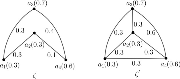
Example 4

Consider the fuzzy graphs $\zeta =(\mu ,\tau )$ and ${\zeta }^{\prime }=({\mu }^{\prime },{\tau }^{\prime })$ of Fig. 4. Clearly it is seen that ${\zeta }^{\prime }$ is the completion of $\zeta$. Now using the Definition 5, we have $CF(\zeta )=1.116$ and $CF({\zeta }^{\prime })=4.58$. Therefore $0\le CF(\zeta )\le CF({\zeta }^{\prime })$.

Fig. 4.

Two fuzzy graphs $\zeta$ and its completion ${\zeta }^{\prime }$

Theorem 4

If two fuzzy graphs $\zeta =(\mu ,\tau )$ and ${\zeta }^{\prime }=({\mu }^{\prime },{\tau }^{\prime })$ are isomorphic to each other, then $CF(\zeta )=CF({\zeta }^{\prime })$.

Proof

Consider two fuzzy graphs $\zeta =(\mu ,\tau )$ and ${\zeta }^{\prime }=({\mu }^{\prime },{\tau }^{\prime })$ are isomorphic to each other. The there must exist a bijective mapping f from $\zeta$ to ${\zeta }^{\prime }$ such that $\mu (a_i)={\mu }^{\prime }(f(a_i)),\forall a_i\in {\mu }^{\ast }$ and $\tau (a_i{a}_j)={\tau }^{\prime }(f(a_i{a}_j)),\forall a_i{a}_j\in {\tau }^{\ast }$. Also, $\mid {\mu }^{\ast }\mid =d=\mid {{\mu }^{\prime }}^{\ast }\mid$ and $\mid {\tau }^{\ast }\mid =s=\mid {{\tau }^{\prime }}^{\ast }\mid$. Since $\zeta \cong {\zeta }^{\prime }$, so the strength of a path in $\zeta$ is equal to the strength of a similar path in ${\zeta }^{\prime }$. Then the sum of the strength of the strengths of all paths between $a_i$ and $a_j$ in $\zeta$ is same as that of $f(a_i)f(a_j)$ in ${\zeta }^{\prime }$ i.e., $S{P}_{\mathit{ij}}=S{P}_{\mathit{ij}}^{\prime }$, $\forall a_i,a_j\in {\mu }^{\ast }$ and $\forall f(a_i),f(a_j)\in {{\mu }^{\prime }}^{\ast }$. Therefore

$$\begin{array}{c}\hfill \frac{\mathit{ds}}{d+s}\sum _{\begin{array}{c}{a}_i,a_j\in {\mu }^{\ast }\\ i>j\end{array}}\mu (a_i)\mu (a_j)S{P}_{\mathit{ij}}=\frac{\mathit{ds}}{d+s}\sum _{\begin{array}{c}f(a_i),f(a_j)\in {{\mu }^{\prime }}^{\ast }\\ i>j\end{array}}{\mu }^{\prime }(f(a_i)){\mu }^{\prime }(f(a_j))S{P}_{\mathit{ij}}^{\prime }\end{array}$$

and hence $CF(\zeta )=CF({\zeta }^{\prime })$. $\square$

If the minimum of the membership values of vertices and the sum of the membership values of edges i.e., size of a fuzzy graph are known, then the evaluation of the lower boundary of complexity function motivate us to introduce the following Theorem.

Theorem 5

For a connected fuzzy graph $\zeta =(\mu ,\tau )$, $CF(\zeta )\ge \frac{d}{d+1}{l}^{2}S$, where S denote the size of $\zeta$ and $l=min\{\mu (a_i):a_i\in {\mu }^{\ast }\}$.

Proof

Let $\zeta =(\mu ,\tau )$ be a connected fuzzy graph with $\mid {\mu }^{\ast }\mid =d$, $\mid {\tau }^{\ast }\mid =s$ and $S(\zeta )$ is the size of $\zeta$.

Since $\zeta$ is connected, so $2s\ge d$ i.e., $s\ge \frac{d}{2}$. Again since $\mid {\mu }^{\ast }\mid =d$, so the number of maximum possible edges of $\zeta$ is ${}^d{C}_2=\frac{d(d-1)}{2}$ and hence $s\le \frac{d(d-1)}{2}$. Then $\frac{\mathit{ds}}{d+s}\ge \frac{d\frac{d}{2}}{d+\frac{d(d-1)}{2}}\Rightarrow \frac{\mathit{ds}}{d+s}\ge \frac{d}{d+1}\dots \dots$(I).

Now we know that in a fuzzy graph, the sum of the strengths of all paths between a pair of vertices is not less than the membership value of the edge between those pair of vertices. Then $S{P}_{\mathit{ij}}\ge \tau (a_i{a}_j)$ and hence

$$\begin{array}{cc}& \sum _{\begin{array}{c}{a}_i,a_j\in {\mu }^{\ast }\\ i>j\end{array}}\mu (a_i)\mu (a_j)S{P}_{\mathit{ij}}\ge \sum _{\begin{array}{c}{a}_i{a}_j\in {\tau }^{\ast }\end{array}}{l}^2\tau (a_i{a}_j)\hfill \\ \hfill & \Rightarrow \sum _{\begin{array}{c}{a}_i,a_j\in {\mu }^{\ast }\\ i>j\end{array}}\mu (a_i)\mu (a_j)S{P}_{\mathit{ij}}\ge l^{2}S\dots \dots \text{(II), by Definition}3.\hfill \end{array}$$

From (I) and (II), we have $CF(\zeta )\ge \frac{d}{d+1}{l}^{2}S$. $\square$

Example 5

Consider the fuzzy graph $\zeta$ of Fig. 4. From the Example 4, we have $CF(\zeta )=0.558$. Here $d=4$, $S=0.3+0.3+0.4+0.1=1.1$, $l=min\{0.3,0.3,0.7,0.6\}=0.3$ and $\frac{d}{d+1}{l}^{2}S=0.0792$. Therefore $CF(\zeta )>\frac{d}{d+1}{l}^{2}S$.

Now, consider a connected fuzzy graph $\zeta =(\mu ,\tau )$, $S=$size of $\zeta$ and $m=max\{\mu (a_i);a_i\in {\mu }^{\ast }\}$. Then the inequality $CF(\zeta )\le \frac{d}{d+1}{m}^{2}S$ may not be true. For this, consider the example.

Example 6

If we consider the fuzzy graph $\zeta$ of Fig. 5, then $d=4,s=4,S=0.8$ and $m=max\{\mu (a_i);a_i\in {\mu }^{\ast }\}=1$. So, $CF(\zeta )=2.4$ and $\frac{\mathit{ds}}{d+s}{m}^{2}S=0.64$. Then $CF(\zeta )>\frac{d}{d+1}{m}^{2}S$.

Fig. 5.

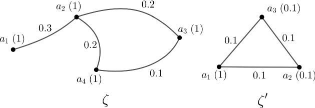
Two fuzzy graphs $\zeta$ and ${\zeta }^{\prime }$

Again, if we consider the fuzzy graph ${\zeta }^{\prime }$ of Fig. 5, then $d=3,s=3,S=0.3$ and $m=max\{\mu (a_i);a_i\in {\mu }^{\ast }\}=1$. So, $CF({\zeta }^{\prime })=0.063$ and $\frac{\mathit{ds}}{d+s}{m}^{2}S=0.225$. Then $CF({\zeta }^{\prime })<\frac{d}{d+1}{m}^{2}S$.

Theorem 6

Let $\zeta =(\mu ,\tau )$ be a fuzzy graph. If $0\le x_1\le x_2\le 1$, then $CF({\zeta }^{x_2})\le CF({\zeta }^{x_1})$.

Proof

Since $x_1\le x_2$, so ${\zeta }^{x_2}$ is a partial fuzzy subgraph of ${\zeta }^{x_1}$ and by Theorem 1 we have, $CF({\zeta }^{x_2})\le CF({\zeta }^{x_1})$. $\square$

Corollary 1

Let $\zeta =(\mu ,\tau )$ be a fuzzy graph. If $0\le x_1\le x_2\le \dots \le x_n\le 1$, then $CF({\zeta }^{x_1})\ge CF({\zeta }^{x_2})\ge \dots \ge CF({\zeta }^{x_n})$.

Theorem 7

Let $\zeta =\mu ,\tau$ be a perfectly regular fuzzy graph such that $deg(a_i)=k$ and $l=\mu (a_i),a_i\in {\mu }^{\ast }$. Then $CF(\zeta )\ge \frac{1}{2}\frac{d^2}{d+1}k{l}^2$.

Proof

Since $\zeta$ is a perfectly regular fuzzy graph, so degree of all the vertices of $\zeta$ are same Cary (2018). So $deg(a_i)=k$ for all $a_i$ in $\zeta$. Also size of $\zeta$ is $S=\frac{\mathit{dk}}{2}$Cary (2018) and $d=\mid {\mu }^{\ast }\mid$. From the Theorem 5, we have

$CF(\zeta )\ge \frac{d}{d+1}{l}^{2}S\ge \frac{d}{d+1}{l}^2\frac{\mathit{dk}}{2}$ and therefore $CF(\zeta )\ge \frac{1}{2}\frac{d^2}{d+1}k{l}^2$. $\square$

Complexity function of fuzzy cycle, tree, regular fuzzy graphs

We have to determine the cycles in which the highest and lowest internet traffic jam occur. Thus in this section, complexity function of fuzzy cycle is given with example. The complexity function of various fuzzy trees and perfectly regular fuzzy graphs are discussed with some of their properties .

If we delete an edge from a fuzzy cycle $\zeta$ then at least one path will be reduced strictly between every pair of vertices. Also the sum of the strengths between every pair of vertices will reduce strictly. So the complexity function of the fuzzy cycle will reduce. Thus we have the proposition.

Proposition 3

Let $\zeta =(\mu ,\tau )$ be a fuzzy cycle and ${\zeta }^{\prime }=(\mu ,{\tau }^{\prime })$, where ${\tau }^{\prime }=\tau -\{e_1\},e_1\in {\tau }^{\ast }$. Then $CF(\zeta )<CF(\zeta )$.

Theorem 8

Let $\zeta =(\mu ,\tau )$ be a fuzzy cycle of the cycle ${\zeta }^{\ast }=({\mu }^{\ast },{\tau }^{\ast })$ such that $\mu$ and $\tau$ both are constant function. If ${\mu }^{\ast }=d$, then $CF(\zeta )=\frac{d^2(d-1)}{2}k{m}^2$, where $m=\mu (a_i),\forall a_i\in {\mu }^{\ast }$ and $k=\tau (a_i{a}_j),\forall a_i{a}_j\in {\tau }^{\ast }$.

Proof

Since $\zeta$ is a fuzzy cycle, so $\zeta$ must be a fuzzy graph. Then the number of vertices and the number of edges in ${\zeta }^{\ast }$ are same i.e., ${\mu }^{\ast }={\tau }^{\ast }=d$.

Since $\zeta$ is a fuzzy cycle, so there are only two paths between every pair of vertices $a_i$ and $a_j$ (see Fig. 6). Now the strengths of these two paths are corresponding minimum of the membership values of the edges, which are lies on these two paths. But, $\tau (a_i{a}_j)=k,\forall a_i{a}_j\in {\tau }^{\ast }$, so $S{P}_{\mathit{ij}}=k+k=2k,\forall a_i,a_j\in {\mu }^{\ast }$. Therefore

$$\begin{array}{cc}\hfill CF(\zeta )=& \frac{d.d}{d+d}\sum _{\begin{array}{c}{a}_i,a_j\in {\mu }^{\ast }\\ i>j\end{array}}\mu (a_i)\mu (a_j)S{P}_{\mathit{ij}}\hfill \\ \hfill =& \frac{d^2}{2d}(m.m.2k){}^d{C}_2=\frac{d^2(d-1)}{2}k{m}^2\hfill \end{array}$$

[$\because$ there are ${}^d{C}_2$ pair of vertices]. $\square$

Fig. 6.

Example of a fuzzy cycle $\zeta$ with $CF(\zeta )=58.8$ for Theorem 8

Theorem 9

Let $\zeta =(\mu ,\tau )$ be a fuzzy tree and $F=(\mu ,{\tau }^{\prime })$ is a maximum fuzzy spanning tree of $\zeta$ such that $F^{\ast }=({\mu }^{\ast },{\tau }^{{\prime }^{\ast }})$ is a tree, $\mid {\mu }^{\ast }\mid =d,\mid {\tau }^{{\prime }^{\ast }}\mid =s$. Then $CF(F)=\frac{1}{2}\frac{d^2(d-1)s}{d+s}{k}^{2}m$, where $k=\mu (a_i),\forall a_i\in {\mu }^{\ast }$ and $m=\tau (a_i{a}_j),\forall a_i{a}_j\in {\tau }^{{\prime }^{\ast }}$.

Proof

Let $F=(\mu ,{\tau }^{\prime })$ be a maximum fuzzy spanning tree of the fuzzy graph $\zeta =(\mu ,\tau )$ and $F^{\ast }=({\mu }^{\ast },{\tau }^{{\prime }^{\ast }})$ be the corresponding tree. Then F must be a fuzzy subgraph of $\zeta$ and F is unique Sunitha and Vijayakumar (1999) (see Fig. 7). Again, since $F^{\ast }$ is a tree, so there is only one path between every pair of vertices in F. Then the total number of different paths in F $={}^d{C}_2[\because \mid {\mu }^{\ast }\mid =d]$ and the strengths of all the paths are $m[\because \tau (a_i{a}_j)=m,\forall a_i{a}_j\in {\tau }^{{\prime }^{\ast }}]$. Therefore

$$\begin{array}{cc}\hfill CF(F)=& \frac{\mathit{ds}}{d+s}\sum _{\begin{array}{c}{a}_i,a_j\in {\mu }^{\ast }\\ i>j\end{array}}\mu (a_i)\mu (a_j)S{P}_{\mathit{ij}}\hfill \\ \hfill =& \frac{\mathit{ds}}{d+s}k.k.m.{}^d{C}_2=\frac{1}{2}\frac{d(d-1)s}{d+s}{k}^{2}m.\hfill \end{array}$$

$\square$

Fig. 7.

An example for Theorem 9 with $CF(\zeta )=3.125$ and $CF(F)=1.667$

Theorem 10

Let $\zeta =(\mu ,\tau )$ be a perfectly regular complete fuzzy graph. Then $CF(\zeta )=\frac{1}{2}\frac{d^2(d-1)}{d+s}{m}^3[(d-2)!e]$, where $m=\mu (a_i),a_i\in {\mu }^{\ast }$ and e is the irrational Euler’s number and third bracket denote the greatest integer function.

Proof

Since $\zeta$ is a perfectly regular fuzzy graph, so $\mu$ must be a constant function Cary (2018). Then the membership values of all the vertices of $\zeta$ are same i.e., $\mu (a_i)=m,\forall a_i\in {\mu }^{\ast }$.

Again, since $\zeta$ is complete, so $\tau (a_i{a}_j)=min\{\mu (a_i),\mu (a_j),\forall a_i{a}_j\in {\tau }^{\ast }\}=min\{m,m\}=m$.

Therefore strengths of all the paths between every pair of vertices in $\zeta$ is m. Since ${\zeta }^{\ast }$ is complete graph, so there are $[(d-2)!e]$ number of paths between every pair of vertices in ${\zeta }^{\ast }$ Harris et al. (2008) and hence $\zeta$. Then $S{P}_{\mathit{ij}}=[(d-2)!e]m,\forall a_i,a_j\in {\mu }^{\ast }$. Therefore

$$\begin{array}{cc}\hfill CF(\zeta )=& \frac{\mathit{ds}}{d+s}\sum _{\begin{array}{c}{a}_i,a_j\in {\mu }^{\ast }\\ i>j\end{array}}\mu (a_i)\mu (a_j)S{P}_{\mathit{ij}}=\frac{\mathit{ds}}{d+s}{}^d{C}_2.m.m.[(d-2!e)]m\hfill \\ \hfill =& \frac{1}{2}\frac{d^2(d-1)}{d+s}{m}^3[(d-2)!e],[\because \text{there are}{}^d{C}_2\text{pair of vertices in}{\zeta }^{\ast }].\hfill \end{array}$$

$\square$

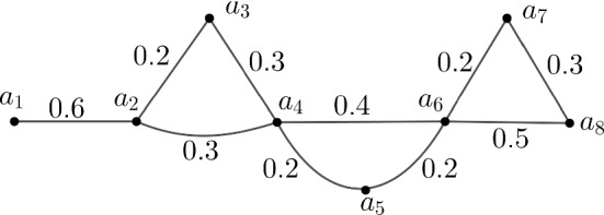
Example 7

Let $\zeta$ be a fuzzy graph (see Fig. 8) with ${\mu }^{\ast }=\{a_1,a_2,a_3,a_4,a_5,a_6,a_7,a_8\},\mu (a_i)=1,\forall a_i\in {\mu }^{\ast }$ and $\tau (a_1{a}_2)=0.6,\tau (a_2{a}_3)=0.2,\tau (a_2{a}_4)=0.3,\tau (a_3{a}_4)=0.3,\tau (a_4{a}_5)=0.2,\tau (a_4{a}_6)=0.4,\tau (a_5{a}_6)=0.2,\tau (a_6{a}_7)=0.2,\tau (a_6{a}_8)=0.5,\tau (a_7{a}_8)=0.3$. So $d=8,s=10$.

Fig. 8.

Fuzzy graph $\zeta$ with membership values of vertices are as 1

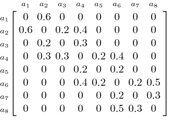
The above matrix is the matrix form of the edges of the fuzzy graph $\zeta$ of Fig. 8. The matrix form of the sum of strengths of all paths between every pair of vertices of $\zeta$ is given below as :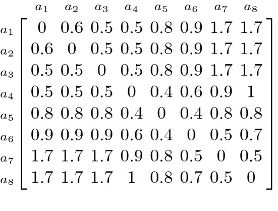

$$\begin{array}{cc}\hfill CF(\zeta )=& \frac{\mathit{ds}}{d+s}(sumofalltheupperorlower\hfill \\ \hfill & triangularentriesoftheabovematrix)\hfill \\ \hfill =& \frac{80}{18}\times 25=111.11\text{(approximate)}.\hfill \end{array}$$

Applications of complexity function of fuzzy graph

Determination of most effected COVID-19 cycle between countries

Description of model

The COVID-19 pandemic began in the late 2019 in Wuhan, China with an infectious virus that is converted version of the Corona virus. China closed the city of Wuhan in late January and by March, 2020, the country effectively controlled the spread of this epidemic, not only to other cities in the country but also to Wuhan. However, the Earth was connected by land, air and sea routs. The virus spread through out the world. In March, 2020 the Western countries were most effected by COVID-19. Governments in the United State of America, Europe and some Asian countries including India have located their countries considering closing. It has created the impression so that most developed countries around the world are panicking against the virus outbreak. It is unclear just how infectious the Corona virus is. It seems to spread from person to person in close contact. When someone coughs or sneezes with virus, it can spread by the release of respiratory tract. If a person touches a surface by a virus and touches his face, nose or eyes, it can also spread. Therefore, the Corona virus can spread from a country to another country mainly by communication (traveling by plane and ship, export and import of animal and foods, etc).

Representation of membership values

Most of the countries were affected by COVID-19 within April, 2020. Here we consider top five COVID-19 affected countries within that time and their graphical representation of transmission due to intercommunications. All the data are taken from Mahapatra et al. (2021) and the website (https://www.worldmeters.info/coronavirus/) dated 4th April, 2020. These five countries are USA, Spain, Italy, China, Germany which represents the vertices $a_1,a_2,a_3,a_4,a_5$ of the fuzzy graph $\zeta$ of Fig. 9. The membership values of vertices are given in Table 1. The chances of spreading virus reached the highest level due to the maximum communication between countries. For maximum communication between countries the membership values of the edges is equal to the minimum of the membership values of corresponding edges of $\zeta$. So, $\tau (a_1{a}_2)=min\{\mu (a_1),\mu (a_2)\}=0.46$. Similarly, $\tau (a_1{a}_3)=0.46$, $\tau (a_1{a}_4)=0.32$, $\tau (a_1{a}_5)=0.35$, $\tau (a_2{a}_3)=0.46$, $\tau (a_2{a}_4)=0.32$, $\tau (a_2{a}_5)=0.35$, $\tau (a_3{a}_4)=0.32$, $\tau (a_3{a}_5)=0.35$, $\tau (a_4{a}_5)=0.32$.

Fig. 9.

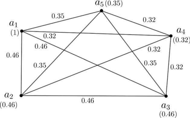
A fuzzy graph $\zeta$ of five COVID-19 affected countries

Table 1.

Five most affected countries by COVID-19 and no. of cases Mahapatra et al. (2021)

Countries (vertices)	Total cases	Normalized score	Membership value of vertices
USA ($a_1$)	258409	1	$\mu (a_1)=$1
Spain ($a_2$)	117710	0.46	$\mu (a_2)=$0.46
Italy ($a_3$)	119827	0.46	$\mu (a_3)=$0.46
China ($a_4$)	81620	0.32	$\mu (a_4)=$0.32
Germany ($a_5$)	89451	0.35	$\mu (a_5)=$0.35

To determine the most effected cycles, the complexity function of all the longest cycles of $\zeta$ need to be find out. There are many cycles in $\zeta$. The highest length of a cycle in $\zeta$ is 5. Here, $\zeta$ is a complete fuzzy graph. The strengths of paths between every pair of vertices depend on the edge membership values. So for computing complexity function, $S{P}_{\mathit{ij}}$ is maximum if the strengths of the paths i.e., membership values of the edges on the paths are maximum. The membership value of the three edges $a_1{a}_2,a_1{a}_3,a_2{a}_3$ are 0.46 is maximum of the edge membership values of $\zeta$. So, we have to find out complexity function of those cycles of length 5 which contains the maximum number of edges from $a_1{a}_2,a_1{a}_3,a_2{a}_3$. A cycle of length 5 contains at most two edges of $a_1{a}_2,a_1{a}_3,a_2{a}_3$. There are only six cycles in $\zeta$ of length 5 contains two of the edge $a_1{a}_2,a_1{a}_3,a_2{a}_3$ which are $a_1-a_2-a_3-a_4-a_5-a_1$ ($C_1$ cycle) shown in Fig. 10, $a_1-a_2-a_3-a_5-a_4-a_1$ ($C_2$ cycle) shown in Fig. 11, $a_3-a_1-a_2-a_5-a_4-a_3$ ($C_3$ cycle), $a_3-a_1-a_2-a_4-a_5-a_3$ ($C_4$ cycle), $a_2-a_3-a_1-a_5-a_4-a_2$ ($C_5$ cycle), $a_2-a_3-a_1-a_4-a_5-a_2$ ($C_6$ cycle).

Fig. 10.

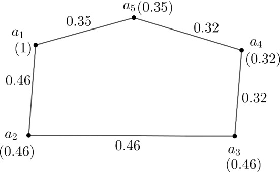
A cycle $C_1$ of the fuzzy graph $\zeta$ of Fig. 9

Fig. 11.

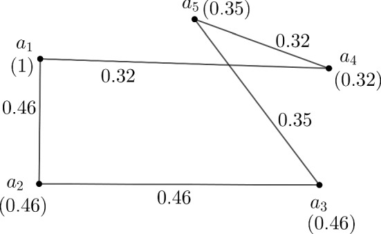
Another cycle $C_2$ of the fuzzy graph $\zeta$ of Fig. 9

$CF(C_1)=\frac{5\times 5}{5+5}(0.78+0.78+0.64+0.67+0.78+0.64+0.67+0.64+0.67+0.64)=17.275$. Similarly, $CF(C_2)=CF(C_3)=CF(C_4)=CF(C_5)=CF(C_6)=17.275$.

Since the values of the complexity function of all the cycles $C_1,C_2,C_3,C_4,C_5,C_6$ of the fuzzy graph $\zeta$ are equal, therefore all these cycles are the most effected and communicated cycles in which the virus COVID-19 mostly spread. Hence, these five cycles $a_1-a_2-a_3-a_4-a_5-a_1$, $a_1-a_2-a_3-a_5-a_4-a_1$, $a_3-a_1-a_2-a_5-a_4-a_3$, $a_3-a_1-a_2-a_4-a_5-a_3$, $a_2-a_3-a_1-a_5-a_4-a_2$, $a_2-a_3-a_1-a_4-a_5-a_2$ are the most effected cycle for spreading the virus COVID-19.

Estimation of busiest internet routing path using complexity function

Model description

Network traffic is increasing because of the internet usage that surrounds our daily lives. User always expect better quality service from network providers. To increase demand and address service expectation, the network operators looking for better utilize underlying topological functions to reduce traffic input and traffic delays, input and latency. Specially, a common practice is load balancing network flow along multiple paths. Routing is only process to select a route for traffic from a single or multiple networks. Obviously, routing takes place on several kind of networks such as mobile tower network, computer networks, traffic signal networks. Choosing the best route through path selection involves applying one route metric to other multiple routes. Multi path route techniques enable the use of multiple alternative paths.

Interpretation of membership values

Suppose we need to cover through towers of mobile phone network and also each village has at least one network tower. This situation can be controlled by graph theory. If a tower can be placed on a village to covers the surrounding villages, then it is connected by an edge. But there is an important think is to found out most effective paths for complexity measure. In Mariappan et al. (2019), a network of five villages is considered having mobile towers. In every village there is a tower placed area, which is denoted by a vertex. The membership values of vertices represents the maximum capacity of the towers in unit. The membership values of edges represents the strength of mobile signal between the corresponding vertices i.e., towers. Now, using the complexity function of fuzzy graph we will determine the most effective paths. Consider the fuzzy graph $\zeta =(\mu ,\tau )$ for the corresponding mobile networks, which is shown in Fig. 12. Here ${\mu }^{\ast }=\{a_1,a_2,a_3,a_4,a_5\}$ and ${\tau }^{\ast }=\{a_1{a}_2,a_1{a}_4,a_2{a}_3,a_2{a}_4,a_3{a}_4,a_3{a}_5,a_4{a}_5\}$. $\mu (a_1)=0.6,\mu (a_2)=0.6,\mu (a_3)=0.7,\mu (a_4)=0.9,\mu (a_5)=0.8$, $\tau (a_1{a}_2)=0.4,\tau (a_1{a}_4)=0.2,\tau (a_2{a}_3)=0.5,\tau (a_2{a}_4)=0.3,\tau (a_3{a}_4)=0.7,\tau (a_3{a}_5)=0.2,\tau (a_4{a}_5)=0.8$.

Fig. 12.

Internet network route between villages

For the fuzzy graph $\zeta =(\mu ,\tau )$ of Fig.12, we have $CF(\zeta -\{a_1\})=8.293,CF(\zeta -\{a_2\})=4.518,CF(\zeta -\{a_3\})=3.624,CF(\zeta -\{a_4\})=1.416,CF(\zeta -\{a_5\})=6.56$. Therefore $CF(\zeta -\{a_1\})>CF(\zeta -\{a_5\})>CF(\zeta -\{a_2\})>CF(\zeta -\{a_3\})>CF(\zeta -\{a_4\})$.

Decision making

The complexity function of the vertex deleted fuzzy subgraph $\zeta -\{a_4\}$ is lowest and $\zeta -\{a_1\}$ is highest. So the vertex $a_4$ i.e., the tower at $a_4$ is the highest effective tower and the vertex $a_1$ i.e., the tower at $a_1$ is the lowest effective tower according to the complexity measure and the path $a_4-a_3-a_2-a_5-a_1$ is the most effective path. Hence the internet load of the tower at $a_4$ is highest and the tower at $a_1$ is lowest and also the path $a_4-a_3-a_2-a_5-a_1$ is the most busiest network route.

Conclusion

A system is called complex if it contains many elements that interact with each other in different ways, for which this interactions somewhere leads to unexpected conjunctions. The purpose of measuring complexity of the above mentioned requirements has been completed. Using these concepts, the complexity function of fuzzy graph with many properties are depicted. Different types of upper and lower boundaries of complexity function of various fuzzy graphs are established. Characterization of complexity function and its measure in fuzzy trees, cycles and regular fuzzy graphs are obtained. Two applications of these research work are obtained to find most effected cycle by COVID-19 and busiest internet routing paths.

Declarations

Conflict of interest

The authors declare that they have no conflict of interest.

Ethical approval

This article does not contain any studies with human participants or animals performed by any of the authors.

References

- Bertz SH. A mathematical model of molecular complexity. In: King RB, editor. Chemical applications of topology and graph theory. Amsterdam: Elsevier; 1987. pp. 206–221. [Google Scholar]
- Bhutani KR, Rosenfeld A. Fuzzy end node in fuzzy graphs. Inf Sci. 2003;152:323–326. doi: 10.1016/S0020-0255(03)00078-1. [DOI] [Google Scholar]
- Bhutani KR, Rosenfeld A. Strong arc in fuzzy graphs. Inf Sci. 2003;152:319–322. doi: 10.1016/S0020-0255(02)00411-5. [DOI] [Google Scholar]
- Binu M, Mathew S, Mordeson JN. Connectivity index of a fuzzy graph and its application to human trafficking. Fuzzy Sets Syst. 2019;360:117–136. doi: 10.1016/j.fss.2018.06.007. [DOI] [Google Scholar]
- Binu M, Mathew S, Mordeson JN. Wiener index of a fuzzy graph and application to illegal immigration networks. Fuzzy Sets Syst. 2020;384:132–147. doi: 10.1016/j.fss.2019.01.022. [DOI] [Google Scholar]
- Borzooei RA, Rashmanlou H. Degree and total degree of edges in bipolar fuzzy graphs with application. J Intell Fuzzy Syst. 2016;30(6):3271–3280. doi: 10.3233/IFS-152075. [DOI] [Google Scholar]
- Cary M. Perfectly regular and perfectly edge-regular fuzzy graphs. Ann Pure Appl Math. 2018;16(2):461–469. doi: 10.22457/apam.v16n2a24. [DOI] [Google Scholar]
- Dehmer M, Chen Z, Streib FE, Tripathi S, Mowshowitz A, Levitchi A, Feng L, Shi Y, Tao J. Measuring the complexity of directed graphs: a polynomial based approach. PLOS One. 2019;14(11):e0223745. doi: 10.1371/journal.pone.0223745. [DOI] [PMC free article] [PubMed] [Google Scholar]
- Dudek WA, Talebi AA. Operation on level graph of bipolar fuzzy graphs. Buletin Academiel de Stiinte A Republic Moldova Matemtica. 2016;2(8):107–124. [Google Scholar]
- Gani AN, Ahamed MB. Order and size in fuzzy graph. Bull Pure Appl Sci. 2003;22E(1):145–148. [Google Scholar]
- Ghorai G, Jacob K. Recent developments on the basics of fuzzy graph theory. In: Pal M, Samanta S, Pal A, editors. Handbook of research on advanced applications of graph theory in modern society. United States: IGI Global; 2019. [Google Scholar]
- Ghorai G, Pal M. Some isomorphic properties of -polar fuzzy graphs with applications. SpringerPlus. 2016;5(1):2104. doi: 10.1186/s40064-016-3783-z. [DOI] [PMC free article] [PubMed] [Google Scholar]
- Harris J, Hirst JL, Mosinghoff M. Combinatorics and graph theory. New York: Springer; 2008. [Google Scholar]
- Lakdashti A, Rashmanlou H, Borzooei RA, Samanta S, Pal M. New concepts of bipolar fuzzy graphs. J Multiple-Valued Logic Soft Comput. 2019;33(1–2):117–133. [Google Scholar]
- Mahapatra R, Samanta S, Pal M, Lee J, Khan SK, Naseem U, Bhadoria RS. Colouring of COVID-19 affected region based on fuzzy directed graphs. Comput Mater Continua. 2021;68(1):1219–1233. doi: 10.32604/cmc.2021.015590. [DOI] [Google Scholar]
- Mariappan S, Ramalingam S, Raman S, Turan GB. Domination integrity and efficient fuzzy graphs. Neural Comput Appl. 2019;32:10263–10273. doi: 10.1007/s00521-019-04563-5. [DOI] [Google Scholar]
- Mathew S, Sunitha MS. Types of arcs in a fuzzy graph. Inf Sci. 2009;179(11):1760–1768. doi: 10.1016/j.ins.2009.01.003. [DOI] [Google Scholar]
- Mathew S, Mordeson JN, Malik D. Fuzzy graph theory. Berlin: Springer; 2018. [Google Scholar]
- Mathew S, Yang HL, Mathew JK. Saturation in fuzzy graphs. New Math Nat Comput. 2018;14(1):113–128. doi: 10.1142/S1793005718500084. [DOI] [Google Scholar]
- Minoli D (1975) Combinatorial graph complexity, Atti della Accademia Nazionale dei Lincei. Class di Scienze Fisiche, Matematiche e Naturali. Rendiconti, 59(6), 651-661
- Mordeson JN, Nair PS. Fuzzy graphs and fuzzy hypergraphs. Germany: Physica-Verlag; 2000. [Google Scholar]
- Mordeson JN, Peng CS. Operation on fuzzy graphs. Inf Sci. 1994;79:159–170. doi: 10.1016/0020-0255(94)90116-3. [DOI] [Google Scholar]
- Mordeson JN, Mathew S, Malik D. Fuzzy graph theory with applications to human trafficking. Berlin: Springer; 2018. [Google Scholar]
- Mordeson JN, Mathew S, Malik DS. Generalized fuzzy relations. New Math Nat Comput. 2018;14(2):187–202. doi: 10.1142/S1793005718500126. [DOI] [Google Scholar]
- Mowshowitz A. Entropy and the complexity of graphs: I. an index of the relative complexity of a graph. Bull Math Biophys. 1968;30:175–204. doi: 10.1007/BF02476948. [DOI] [PubMed] [Google Scholar]
- Nagoorgani A, Hussain RJ. Connected and global domination of fuzzy graph. Bull Pure Appl Sci. 2008;27E(2):1–11. [Google Scholar]
- Poulik S, Ghorai G. Detour g-interior nodes and detour g-boundary nodes in bipolar fuzzy graph with applications. Hacettepe J Math Stat. 2020;49(1):106–119. [Google Scholar]
- Poulik S, Ghorai G. Note on bipolar fuzzy graphs with applications. Knowl Based Syst. 2020;192:1–5. doi: 10.1016/j.knosys.2019.105315. [DOI] [Google Scholar]
- Poulik S, Ghorai G (2021) Determination of journeys order based on graph’s Wiener absolute index with bipolar fuzzy information. Inf Sci 545:608–619
- Poulik S, Ghorai G. Certain indices of graphs under bipolar fuzzy environment with applications. Soft Comput. 2020;24(7):5119–5131. doi: 10.1007/s00500-019-04265-z. [DOI] [Google Scholar]
- Poulik S, Ghorai G, Xin Q. Pragmatic results in Taiwan education system based IVFG & IVNG. Soft Comput. 2020 doi: 10.1007/s00500-020-05180-4. [DOI] [Google Scholar]
- Rashmanlou H, Samanta S, Pal M, Borzooei RA. Bipolar fuzzy graphs with categorical properties. Int J Comput Intell Syst. 2015;8(5):808–818. doi: 10.1080/18756891.2015.1063243. [DOI] [Google Scholar]
- Rashmanlou H, Samanta S, Pal M, Borzooei RA. Product of Bipolar fuzzy graphs and their degrees. Int J Gen Syst. 2016;45(1):1–14. doi: 10.1080/03081079.2015.1072521. [DOI] [Google Scholar]
- Rosenfield R. Fuzzy graphs. In: Zadeh LA, Fu KS, Shimura M, editors. Fuzzy sets and their application. New York: Academic press; 1975. pp. 77–95. [Google Scholar]
- Sunitha MS, Vijayakumar A. A characterization of fuzzy trees. Inf Sci. 1999;113(3–4):293–300. doi: 10.1016/S0020-0255(98)10066-X. [DOI] [Google Scholar]
- Talebi AA. Cayley fuzzy graphs on the fuzzy groups. Comput Appl Math. 2018;37:4611–4632. doi: 10.1007/s40314-018-0587-5. [DOI] [Google Scholar]
- Talebi AA, Ghassemi M, Rashmanlou H. New concepts of irregular-intuitionistic fuzzy graphs with applications. Ann Univ Math Comput Sci Ser. 2020;47(2):226–243. [Google Scholar]
- Talebi AA, Ghassemi M, Rashmanlou H, Broum S. Novel properties of edge irregular single valued neutrosophic graphs. Neutrosophic Sets Syst. 2021;43:255–279. [Google Scholar]
- Thirunavukarasu P, Suresh R, Viswanathan KK. Energy of a complex fuzzy graph. Int J Math Sci Eng Appl. 2016;10(1):243–248. [Google Scholar]
- Todeschini R, Consonni V. Handbook of molecular descriptors. London: Wiley; 2000. [Google Scholar]
- Trucco E. A note on the information content of graphs. Bull Math Biophys. 1956;18:129–135. doi: 10.1007/BF02477836. [DOI] [Google Scholar]
- Yeh RT, Bang SY. Fuzzy relations, fuzzy graphs and their applications to clustering analysis. In: Zadeh LA, Fu KS, Shimura M, editors. Fuzzy sets and their applications. London: Academic Press; 1975. pp. 125–149. [Google Scholar]
- Zadeh LA. Fuzzy sets. Inf Control. 1965;8:338–353. doi: 10.1016/S0019-9958(65)90241-X. [DOI] [Google Scholar]