

Graphical abstract

Keywords: Temperature, Neural network, Equatorial Africa, COVID-19 lockdown, Time-series, Sunspot number
Abstract
We present interesting application of artificial intelligence for investigating effect of the COVID-19 lockdown on 3-dimensional temperature variation across Nigeria (2°–15° E, 4°–14° N), in equatorial Africa. Artificial neural networks were trained to learn time-series temperature variation patterns using radio occultation measurements of atmospheric temperature from the Constellation Observing System for Meteorology, Ionosphere, and Climate (COSMIC). Data used for training, validation and testing of the neural networks covered period prior to the lockdown. There was also an investigation into the viability of solar activity indicator (represented by the sunspot number) as an input for the process. The results indicated that including the sunspot number as an input for the training did not improve the network prediction accuracy. The trained network was then used to predict values for the lockdown period. Since the network was trained using pre-lockdown dataset, predictions from the network are regarded as expected temperatures, should there have been no lockdown. By comparing with the actual COSMIC measurements during the lockdown period, effects of the lockdown on atmospheric temperatures were deduced. In overall, the mean altitudinal temperatures rose by about 1.1 °C above expected values during the lockdown. An altitudinal breakdown, at 1 km resolution, reveals that the values were typically below 0.5 °C at most of the altitudes, but exceeded 1 °C at 28 and 29 km altitudes. The temperatures were also observed to drop below expected values at altitudes of 0–2 km, and 17–20 km.
1. Introduction
In December 2019, the global community found itself in the wake of the spread of the novel coronavirus (CoV) disease 2019 (COVID-19) that has lead to the death of over 3.4 million human lives across the world (Worldometers, 2021). The rapid and almost uncontrolled spread of the disease, among other reasons, made World Health Organization (WHO) to declare it a health emergency and a global pandemic. The consequence was a quick reduction of societal activities.
The Nigerian government declared schools at all levels closed from 20 March to 24 March 2020 as a temporary measure to curb the spread of COVID-19. A total lockdown was later imposed from 25 March which lasted to 19 August 2020 (Reuters, 2021). The first phase of the lockdown was announced by the President on 27 April 2020 with effect from May 4 to 17, and later extended to 1 June 2020 (Ibrahim et al., 2020). During this phase, there was strict sit-at-home order and compliance for all activities, except essential services. The second phase of the gradual easing of the lockdown commenced on 2 June 2020 and lasted for four weeks, which ended on June 29 according to the officer in charge, the Secretary to the Government of the Federation (Ibrahim et al., 2020, Oyeyemi, 2020). Some of the activities that remained prohibited are interstate movement except for essential services, local and international airport operations except for emergency flights, and gatherings of more than 20 people except for workplaces. Ibrahim et al. (2020) contains full details of the further measures detailed in the second phase. The third phase of the easing of lockdown in Nigeria was announced on 30 June 2020 following the approval of the 5th interim report of the Presidential Task Force on COVID-19 by the Nigerian President (Ibrahim et al., 2020). This phase was initially expected to last for four weeks from 30 June to 27 July 2020, but was extended to beyond the month of September (Ibrahim et al., 2020, LEGIST, 2021). Some of the modifications made on phase two include the gradual reopening of airports for local flights “based on close monitoring”, resumption of schools for returning students in secondary schools with the graduating set to resume first, and the lifting of the ban on interstate travels. Nationwide curfew was maintained from 10 pm to 4 am while the use of facemasks in public places also remains mandatory and now punishable by law (Ibrahim et al., 2020, Omilana, 2020).
There are already numerous studies which have investigated the impact of the atmosphere on spread of the COVID-19 virus, but there is paucity of research that has investigated the impact of the COVID-19 lockdown on the atmosphere. In one of such studies, Mandal and Pal (2020) used a relatively few days of satellite images and field derived data in the Indian region of the Dwarka River Basin during pre and lockdown periods to show that the land surface temperatures reduced by about 3–5 °C in the region. For another Indian region of Kolkata, Chowdhuri et al. (2021) conducted a trend analysis of the maximum, minimum and average temperatures during the lockdown period (24 March to 6 May) in 2020 and at the same time for the previous four years, from 2016 to 2019. Their results showed that the increasing trend of daily minimum, average, and maximum temperatures during the lockdown period of March to May 2020 are respectively 0.091 °C, 0.118 °C, and 0.106 °C. These values are the lowest when compared to values of the four prior years, indicating that, in overall, the lockdown caused the temperatures to decrease in the region. In Raipur city of India, Guha and Govil (2021) examined changes in the land surface temperature during the lockdown period by comparing data obtained during the period with data obtained during the earlier periods (2013–2019). Their results also showed that the land surface temperature was reduced during the lockdown.
In a research that reported counterintuitive findings, Gettelman et al. (2021) used simulations from two Earth System Models (the Community Earth System Model 2 (CESM2) and ECHAM6.3–HAM2.3 model (Neubauer et al., 2019)) to show that the impacts of aerosol changes on regional land surface temperatures could cause temperatures to increase by up to + 0.3 K. Their simulation results also showed that the peak impact of aerosol changes on global surface temperature is a small increase (+ 0.03 K). They however noted that aerosol changes are the largest contributions to radiative forcing and temperature changes as a result of COVID-19 affected emissions, larger than ozone, CO2 and contrail effects.
In Africa generally, there is lacking research on impact of the COVID-19 lockdown on the atmosphere. The present study is the first in the region to present a comprehensive investigation on impact of the COVID-19 lockdown on the atmospheric temperatures. The method of artificial neural network is applied to 3-dimensional temperature measurements obtained from the Constellation Observing System for Meteorology, Ionosphere, and Climate (COSMIC). Artificial neural networks (ANNs) are used to learn time series variations of the 3-dimensional atmospheric temperature parameter for more than 13 years prior to the period of the COVID-19 lockdown in 2020. The trained networks are used to predict the expected temperature trends for the lockdown period in 2020, assuming no COVID-19 lockdown, and by comparing with the actual measurements, the impact of the lockdown on atmospheric temperatures is estimated. Unlike in other previous studies, the present study also demonstrates impact of the lockdown on temperatures at varying altitudes in the atmosphere, starting from 0.1 to ∼40 km altitude.
ANNs are most suitable for this investigation, considering the big data involved and established capacity of neural networks to learn trends in complex systems (Baboo and Shereef, 2010, Okoh et al., 2019). ANNs have been applied to analyze large and unstructured data, and to carry out functions such as: time series forecasting, data processing, sequence classification, pattern re-orientation and numerical control (Javeed et al., 2018). ANNs have also been demonstrated to be ideal candidates for modeling atmospheric parameters in the region (Fadare, 2009, Id et al., 2015, Kenabatho et al., 2015, Okoh et al., 2015, Okoh et al., 2020). Asides investigating the impact of the COVID-19 lockdown, the ANN technique is considered in this work as a novel approach to model atmospheric temperature for the region in three dimensional space (longitude, latitude, and altitude) as well as time, making it possible to predict/forecast the atmospheric temperature for all given locations in the region, using data that is not simultaneously available for all the locations. This is the first study to present effect of the COVID-19 lockdown on 3-dimensional atmospheric temperature measurements, starting from ground to stratospheric altitudes of about 40 km.
2. Data and methods
Atmospheric temperature data used in this study are radio occultation (RO) measurements from the COSMIC mission. Measurements from both COSMIC I and COSMIC II missions were used. The data were obtained as second level (wetPrf and wetPf2) files from website of the University Corporation for Atmospheric Research (UCAR, https://data.cosmic.ucar.edu/gnss-ro/). Available data from May 2006 to September 2020 were used. Data from the website are available in Tape Archive (TAR) format. The TAR files were first decompressed to extract the NetCDF (Network Common Data Form) files which they contain. Each NetCDF file contains altitudinal profiles of atmospheric parameters like temperature. The altitudinal profiles of temperature extracted from these files were used in this study. The NetCDF files also contain badness flags that indicate whether or not the profiles in each of the NetCDF files passed the quality control checks. Only profiles that passed the quality control checks were used in this study. The “quality control checks” referred here are in the same context as described for the “badness flag” of the wetPrf files in the COSMIC Data Analysis and Archive Center (CDAAC; see https://cdaac-www.cosmic.ucar.edu/cdaac/cgi_bin/fileFormats.cgi?type=wetPrf). In this description, a badness flag of 0 means that the profile passed quality control check, while a badness flag of 1 means that the profile failed the quality control check. Adhikari et al. (2021) contains a detailed description of the processes and criteria involved for determining whether or not a profile passed the quality control check. The total number of profiles that passed quality control checks and used in this study is 19686, and the total number of data points contained in them is 9028733.
Inputs used for the neural network training are mainly time series indicators and 3-dimensional space indicators. For time series indicators, we used hour of the day (in universal time, UT), the day of the year, and the year. For 3-D space indicators, we used longitude (in degrees), latitude (in degrees), and altitude (in km). The hour of the day was introduced to facilitate the neural network’s learning of diurnal variations. The day of the year was introduced to facilitate the network’s learning of seasonal variations, and the year was introduced to facilitate the network’s learning of long-term variations over the years. The 3-D space indicators were respectively introduced to facilitate the network’s learning of spatial variations across the longitudes, latitudes and altitudes. We also tested the effectiveness of the sunspot number (SSN) parameter for temperature modeling. The sunspot number provides a representation of the solar activity which has a cycle of ∼11 years. Over the years, scientists and researchers have argued on the role/significance of solar activity on atmospheric temperatures (e.g. Meadows, 1975, Schwentek and Elling, 1981, Gil-Alana et al., 2014, Scafetta, 2014, El-Borie et al., 2020). To investigate the significance of solar activity for atmospheric temperature modeling, we considered the SSN as an additional input for the neural network training.
For the purpose of numerical continuity from the end of one day to the start of the next day, and from the end of one year to the start of the next year, we employed cyclical components of the Hour of day and Day of year as respectively shown in Eqs. (1), (2).
| (1) |
| (2) |
In all, we therefore considered the following nine input neurons for the neural network training: Year, , , , , Longitude, Latitude, Altitude, and Sunspot number. To investigate the significance of the SSN, we trained two sets of neural networks; in one set, all of the above nine input neurons were used, and in the other set, eight of them (excluding the SSN) were used. Both sets are identical in every way, except that the later set does not include the SSN input neuron. This setup made it possible to evaluate the contribution of the SSN as an input neuron for the networks. The results are demonstrated in the Results and Discussion section.
The feed-forward back-propagation neural network method was used for the training, and the training algorithm used is the Levenberg-Marquardt back-propagation algorithm (Levenberg, 1944). The weight matrices and bias vectors were updated in accordance with the optimization method for this algorithm. The Levenberg-Marquardt back-propagation algorithm is admired because it is fast, less computationally intensive, requires less memory, and efficient in learning (Wilamowski et al., 2001, Kisi and Uncuoglu, 2005, Okoh et al., 2015, Xu and Zhao, 2020).
COSMIC measurements obtained before the COVID-19 lockdown (that is, from May 2006 to December 2019, except April to September 2018) were used for the neural network training, validation and testing. We shall hereafter refer to this dataset as the neural network dataset. Measurements from April to September 2020 were set aside for evaluation of the effect of the lockdown on atmospheric temperatures, and measurements from April to September 2018 were set aside for the purpose of control experiments. The number of data points in the April to September 2018 measurements is 28880, and the number of data points in the April to September 2020 measurements is 3324449. The choice of year 2018 for control experiment dataset is based on the requirement that we need dataset that is similar to that of year 2020. Using data for year 2018 ensures that we retain data for year 2019 in the neural network training dataset, so that the neural networks get to learn the most recent trends prior to the year for which the lockdown evaluation is done.
Prior to the neural network training, the neural network dataset was split in 3 categories: 71.62% for training, 13.63% for validation, and 14.75% for testing. The validation and test datasets were constituted by systemically removing the data for certain days in the years; for the validation dataset, it was the days starting from day number 2 in steps of 7 days to the end of the year, while for the test dataset, it was starting from day number 5 in steps of 7 days to the end of the year. The reason why we chose to constitute the validation and test datasets systemically, rather than randomly, is to ensure that these datasets contain a good distribution of data for different years, seasons, times/hours of the days, longitudes, latitudes, and altitudes.
To decide an appropriate number of neurons for the hidden layer, we trained 15 different neural networks that differed in the number of hidden layer neurons assigned to them, starting from 1 in steps of 1–15. Decision of the appropriate number of hidden layer neurons was based on criteria of minimizing the neural network prediction errors; the smaller the prediction error, the better. The validation dataset was used during evaluation of the neural network prediction errors; each of the 15 networks were simulated to predict the atmospheric temperatures corresponding to the validation dataset, and thereafter the mean absolute errors (MAEs) were computed using Eq. (3).
| (3) |
The s and the s are respectively the COSMIC measurements and corresponding neural network predictions, and n is the total number of COSMIC measurements. Results of the MAEs are presented in the Results and Discussion section.
The Levenberg-Marquardt based neural network training was implemented on MATLAB using the trainlm function on MATLAB's neural network toolbox. Eqs. (4), (5) respectively indicate the transfer functions applied between the input-hidden and hidden-output layers.
| (4) |
| (5) |
, , and are respectively the input, the hidden, and the output layer matrices. and are respectively the input and hidden layer weight matrices. and are respectively the bias vectors for the input and hidden layer. The layer weight matrices and bias vectors for the finally adopted neural network are as contained in Okoh et al. (2021). The flowchart in Fig. 1 contains a descriptive summary of the processes employed in this study.
Fig. 1.

Flowchart containing descriptive summary of processes employed in this study.
3. Results and discussions
3.1. Investigating significance of sunspot number and deciding number of neurons for the hidden layer
To investigate the significance of SSN for atmospheric temperature prediction, we trained two sets of neural network that are identical in every way except that the SSN was included as input neuron in one set, and excluded in the other set. For each set, we trained 15 neural networks that varied in their number of hidden layer neurons, starting from 1 to 15 in steps of 1. The performance of each network is evaluated based on MAEs computed from the networks’ predictions of the validation dataset. The results are as shown in Fig. 2 .
Fig. 2.
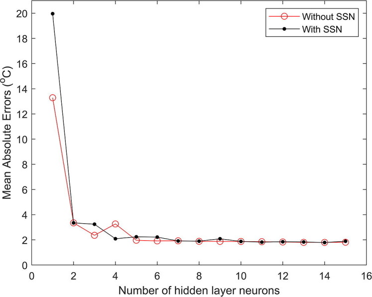
MAEs computed for the neural networks, with and without SSN input neuron, and varying the number of hidden layer neurons from 1 to 15 in steps of 1.
The optimal network is decided based on criteria of minimizing the MAEs. Fig. 2 shows that, for majority of the cases, the performances of both sets of neural networks are identical; the MAEs for the networks with and without SSN included are similar (e.g., for networks with number of hidden layer neurons = 2, 7, 8, 10, 11, 12, 13, 14, and 15). The network with SSN included as input neuron is better than the one without SSN included only for the networks with 4 hidden layer neurons. The networks without SSN included as input neuron are better than the ones with SSN included for the networks with number of hidden layer neurons = 1, 3, 5, 6 and 9. The differences for the latter cases are however small (typically less than 1 °C, except for the obnoxious networks with only 1 number of hidden layer neuron). The averages of the MAEs (excluding the unreliable networks with only 1 number of hidden layer neuron) are respectively 2.15 °C and 2.11 °C for the set of networks with and without SSN included as input neuron. The results indicate that the networks without SSN are slightly better than the networks with SSN included as input neuron. The 0.04 °C difference is however insignificant compared to the average MAEs. We conclude, in general, that there is no significant difference between the MAEs of both sets of neural networks, especially considering that we will be dealing with the networks which give the smallest MAEs. The MAEs for these networks are very much identical. Precisely, we have chosen the networks with 14 hidden layer neurons since they gave the least prediction errors (MAEs = 1.80 °C for both the set with and without SSN included as input neuron). Statistical test on the significance of the difference between predictions of the neural networks (with and without sunspot numbers) for the final versions of the neural networks (14 hidden layer neurons) was also conducted. The two-sample t-test (implemented on MATLAB as the “ttest2” function) was applied on two vectors which independently represent the predictions from the final versions of the neural networks with and without sunspot numbers. The test analysis returned a test decision, h = 0, which indicates that the predictions from the two neural networks do not differ significantly at the default 5% significance level.
Asides the foregoing slight MAE advantage of the networks without SSN inputs over the networks with SSN inputs, the networks without SSN inputs offer some additional benefits; they are easier to implement, they are faster during user runtimes, and they make less use of computational resources. The reason is that the number of input layer neurons is less by 1, and therefore the dimensionality of the network is correspondingly lower. Furthermore, since the network obtained from this study is intended for operational forecasting, the network without SSN inputs is expected to provide more accuracy during forecasts. The reason is that the SSN parameter requires to be measured prior to being made available for the network prediction. Since the measurement cannot be done ahead of the future, a reasonable solution will be to obtain the forecast SSN values from SSN models. Such SSN models do possess inherent prediction errors which will add to the overall error of the atmospheric temperature model. This is the reason we have finally adopted the network without SSN input neuron. We shall refer to this network henceforth as the validated network. The implementation of this network is contained as a MATLAB function in Okoh et al. (2021).
3.2. Neural network testing and error analysis
The test dataset reserved prior to neural network training was used in this section to test performance of the validated network, and to provide information on error analysis for the network. The formula in Eq. (3) was used to compute MAEs for predictions of the network which correspond to the test dataset. The analysis of error is presented as a function of altitude since the most dominant variation of the atmospheric temperature is altitudinal. The test dataset was binned at 1 km interval, starting from 0 to 40 km. For each bin, the MAE is computed based on the test dataset. Result of the MAE as a function of altitude is shown in Fig. 3 . The figure shows that typical prediction errors of the network are in the range of between 0.7 and 2.3 °C. The prediction errors are observed to be greater at altitudes of about 0 km, 18 km, and 36 km. These altitudes are expected to be similar altitudes where the atmospheric temperature shows greater variability because model prediction accuracies are known to be influenced by variability of the modeled parameter (e.g., Schemper, 2003, Diederen and Schultz, 2015, Okoh et al., 2020). To simulate the degree of temperature variability at different altitudes, we computed the standard deviations (STDs) for observations at each of the 1 km bins introduced earlier. The plot marked “STD” in Fig. 3 shows altitudinal variation of the computed standard deviations. Similar to the plot of MAEs, the plot of STDs shows that variability of the atmospheric temperatures are greater at around 0 km, 18 km, and 36 km.
Fig. 3.
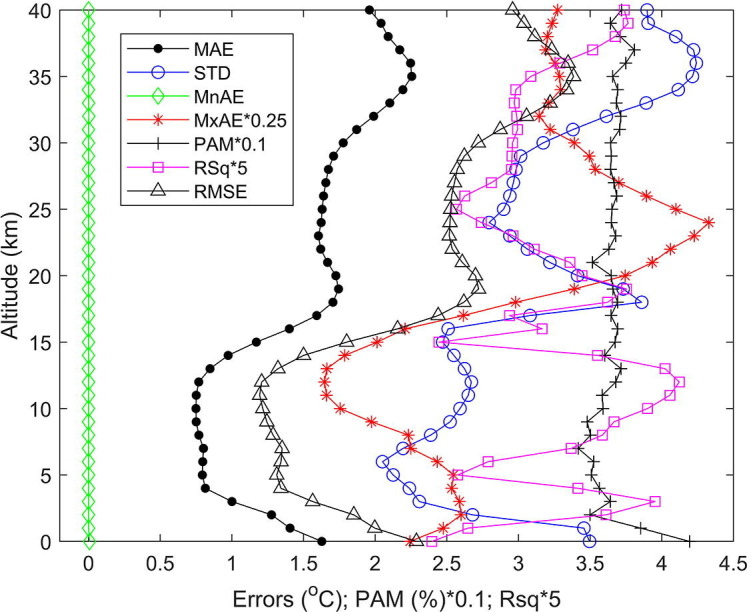
Altitudinal profiles of the Mean Absolute Errors (MAE), the Minimum Absolute Errors (MnAE), the Maximum Absolute Errors (MxAE), the standard deviations of the atmospheric temperatures (STD), the Coefficients of Determination (RSq), the Percentages of data points with an absolute error higher than the MAE (PAM), and the Root-Mean-Square Errors (RMSE), binned at 1 km interval.
Fig. 3 also contains altitudinal profiles of the Minimum Absolute Errors (MnAE), the Maximum Absolute Errors (MxAE), the Coefficients of Determination (RSq), the Percentages of data points with an absolute error higher than the MAE (PAM), and the Root-Mean-Square Errors (RMSE), binned at 1 km interval. The parameters MxAE, RSq, and PAM, are respectively multiplied by factors 0.25, 5, and 0.1 so that their values fit into the scale of Fig. 3. The figure shows that the minimum absolute errors are typically ∼0 at all altitudes, indicating that there are always neural network predictions that are equal to the corresponding COSMIC measurements at all altitudes. The maximum absolute errors are in the range of ∼6 to 17 °C, and the RMSEs are in the range of ∼1 to 3 °C. The shape of the RMSE profile is expectedly similar to the shape of the MAE profile, but the RMSE values are moderately greater than the MAE values, and this is obviously due to the reason that the RMSE systematically penalizes larger errors (Okoh et al., 2019). The PAM values are typically ∼35% to 40%, the mean value for all altitudes is 36.5%, indicating that less than half (∼36.5%) of the data points have absolute errors greater than the MAE. The coefficients of determination are in the range of ∼0.5 to 0.8, indicating that the neural network model does explain greater than 50% of the variability at all altitudes.
Close to Earth surface, the MAE is about 1.6 °C which is similar to, or even less than, typical errors obtained in recent surface temperature modeling efforts. For example, Hyrkkänen et al. (2016) investigated the error characteristics of temperature forecast in Finland for the period 1979–2011. They reported that the rate of root-mean-square errors that had come within a 2.5 °C error threshold had increased from 70% to 85%–90% during the 30 years period, indicating that 2.5 °C was an acceptable value for temperature prediction root-mean-square error. More recently, Seman (2020) demonstrated that MAEs for maximum temperature predictions from the Weather Prediction Center had decreased from about 6.0 °F in 1972 to about 3.3 °F in 2017. Considering the fundamental intervals of the two temperature scales, the 3.3 °F error value can be scaled to an equivalent of about 1.8 °C. In another study that is based on the same region as the present study, Okoh et al. (2015) showed that typical root-mean-square errors for their surface temperature predictions were about 2 °C and less. The 1.6 °C MAE value obtained in the present study is therefore comparatively satisfactory.
3.3. Effect of COVID-19 lockdown on atmospheric temperatures
To investigate the effect of the COVID-19 lockdown (which started in March 2020 in Nigeria), we simulate the neural network predictions for instances corresponding to those in which COSMIC temperature measurements are available during the lockdown period (April to September 2020). It is important to clarify the rationale for this investigation here. The neural network was trained using dataset collected prior to the COVID-19 lockdown, and as such, the neural network predictions do not contain signatures of the COVID-19 lockdown. On the other hand, the COSMIC measurements from April to September 2020 (during the lockdown) will contain expected signatures of the lockdown. By comparing corresponding temperature profiles from the neural network and from the post-lockdown COSMIC measurements, the lockdown effects on atmospheric temperatures are deduced. As a control experiment, we repeat the same process using data of April to September 2018. The purpose is to check that the results we obtain as the lockdown effects are not also contained in the pre-lockdown dataset. Fig. 4 a and b show how the COSMIC measurements compare with the neural network predictions for April to September of years 2018 and 2020 respectively.
Fig. 4.
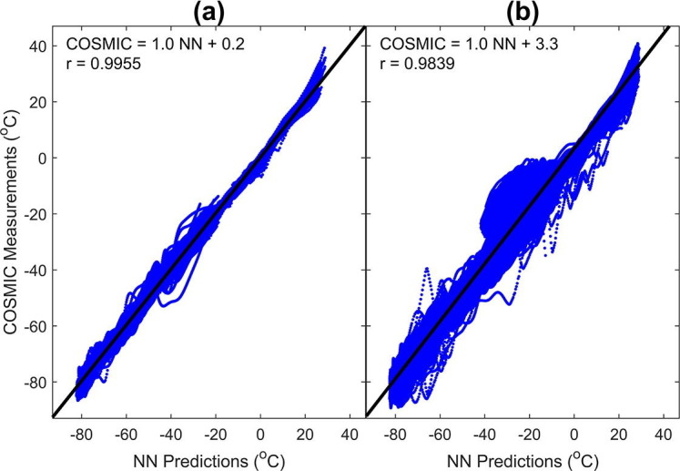
COSMIC temperature measurements versus neural network predictions for the months of April to September in year (a) 2018, and (b) 2020. The black lines are best-fit straight lines for the data points.
The values of correlation coefficient between the COSMIC measurements and neural network predictions are respectively 0.9955 and 0.9839 for the 2018 and 2020 dataset. The coefficients of determination are respectively 0.9911 and 0.9680. These very high correlation coefficient values reveal that the neural network predictions have very identical trends as the COSMIC measurements, although the datasets used here were not used for the neural network trainings. The high correlation coefficient values also signify the high accuracy to which the neural network did learn the temperature variation patterns. The black lines in Fig. 4 represent the best-fit straight lines through the data points. The equations of these lines are respectively given by Eqs. (6), (7) for the 2018 and 2020 dataset.
| (6) |
| (7) |
represents the COSMIC measurements while represents the neural network predictions. In the ideal case that the neural network predictions exactly replicate the COSMIC measurements, we expect to have an equation of the form: , with zero intercept and a slope of 1. Since the equations of the best-fit straight lines are calculated based on distance weights of the points around the majority, a similar ideal equation will be obtained, not only if the neural network predictions are exactly equal to the COSMIC measurements, but also if the distribution of the errors is perfectly Gaussian. This explains why Eq. (6) is ‘almost’ ideal, having a slope of 1.0 and an intercept of 0.2. The ‘close to ideal’ nature of Eq. (6) also tells that the distribution of the neural network prediction errors is almost perfectly Gaussian for the 2018 dataset. This assertion is corroborated by the distribution curve of Fig. 5 c. The scenario gives credence, in our control experiment, to the idea that the neural network predictions are not notably skewed in a particular direction, even for dataset that is not used for training.
Fig. 5.
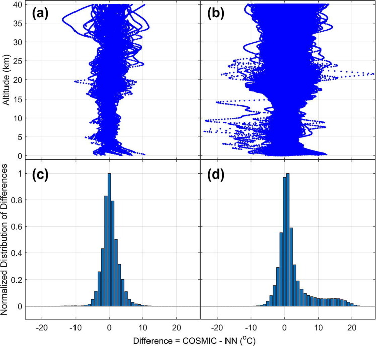
Altitude-based distribution of differences computed between the COSMIC measurements and neural network predictions for the months of April to September of year (a) 2018, and (b) 2020. Normalized distribution of the differences for the months of April to September of year (c) 2018, and (d) 2020.
On the other hand, Eq. (7) shows an intercept of 3.3 °C on the vertical () axis. Interestingly, the slope of the line, however, is still 1.0. The implication is that: for the 2020 dataset, there is typically about 3.3 °C difference between the COSMIC measurements and the neural network predictions. Precisely, the difference is tilted in favor of the COSMIC measurements; the COSMIC measurements are typically greater than the neural network predictions by about 3.3 °C. This is the first indication we get from our work that the atmospheric temperatures did increase during the 2020 lockdown period, compared to modeling that is based on pre-lockdown measurements.
It is important to emphasize that the 3.3 °C difference obtained from the foregoing is based on all altitudes in the profiles from 0 to 40 km. In order to conduct an altitude-dependent investigation, we first compute the differences as functions of altitude. Fig. 5a and b indicate how the differences (computed as COSMIC measurements minus neural network predictions) vary with altitude for the 2018 and 2020 datasets respectively. For reason of the high density of points involved, the distribution density of the differences may not be clearly evident. However, it is noticeable that the distribution of points in Fig. 5a appear to be centered at about 0 °C, but that the distribution of points in Fig. 5b appear to be centered somewhere to the right of 0 °C. This is an indication that there are more of the positive temperature differences than the negative ones in Fig. 5b. To clearly demonstrate any skew in the distribution, we computed the normalized distribution of the differences, shown in Fig. 5c and d, for the 2018 and 2020 datasets respectively. Fig. 5c reveals an almost perfect Gaussian distribution of the differences, which is centered on 0 °C. This means that the greatest majority of the differences are 0 °C, and that there is a comparable drop on both sides, moving away from 0 °C. The implication is that the neural network predictions are in tune with the COSMIC measurements. The scenario is however different in Fig. 5d where the distribution curve is rather centered on 1 °C. There is also clearly evident asymmetry in the shape of the curve; there is an enhanced distribution of points to the right hand side, than to the left hand side (see the lower parts of the curve, for instance). This gives a general sense that the COSMIC measurements during the lockdown are typically greater than the predicted values should there have been no lockdown. For statistical confirmation, we compute the means of “COSMIC measurements minus neural network predictions”. The values are respectively 0.3 and 1.4 °C for the 2018 and 2020 dataset. By regarding the 2018 value of 0.3 °C as the mean error associated with the neural network prediction, we estimate that the lockdown may have caused the mean atmospheric temperatures to increase by about 1.1 °C across altitudes 0 to 40 km.
To get further insight into the altitudinal distribution of the differences, we put the temperature values in 1 km bins. For each bin, we compute the means of “COSMIC measurements minus neural network predictions” for each of the 2018 and 2020 dataset. By regarding the 2018 values as the mean errors associated with the neural network predictions, we estimate effect of the lockdown on the 2020 temperatures by computing differences between the 2020 and 2018 values. The results are illustrated in Fig. 6 a and in Table 1 . The figure and the table illustrate altitudinal variation of the April to September 2020 mean temperature differences, with the neural network mean prediction errors removed. Table 1 also contains additional information on the standard, maximum, and minimum deviations.
Fig. 6.
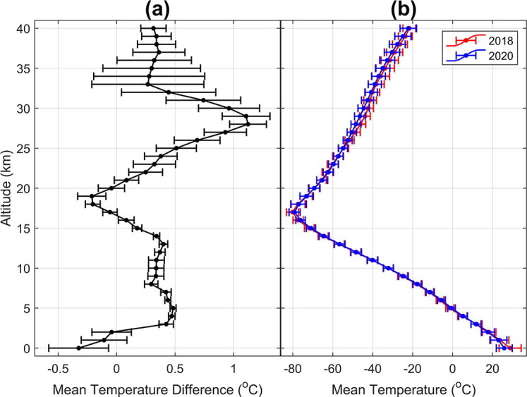
(a) Altitudinal variation of the Mean Temperature Differences for April to September 2020, with the neural network mean prediction errors removed (The neural network mean prediction errors are estimated using the Mean Temperature Differences for April to September 2018), and (b) Altitudinal variation of the Mean Temperatures, computed using dataset for the months of April to September 2018 and April to September 2020. The lengths of the error bars in (a) represent the standard deviations of the differences between the predictions and measurements at each altitude bin.
Table 1.
Descriptive statistics of deviations from the predicted data for 2020 at each altitude bin.
| Altitude bin (km) | Number of data points | Mean of deviations (°C) | Standard deviation (°C) | Maximum deviation (°C) | Minimum deviation (°C) |
|---|---|---|---|---|---|
| 0 | 4138 | −0.3242 | 0.2558 | 12.4229 | −6.1119 |
| 1 | 48,502 | −0.1072 | 0.1954 | 11.9434 | −10.7797 |
| 2 | 76,517 | −0.0424 | 0.1688 | 7.3534 | −15.4474 |
| 3 | 82,311 | 0.4244 | 0.0616 | 5.4326 | −18.2513 |
| 4 | 83,445 | 0.4716 | 0.0278 | 4.2151 | −14.8429 |
| 5 | 83,929 | 0.4830 | 0.0258 | 7.2173 | −16.3855 |
| 6 | 84,199 | 0.4378 | 0.0256 | 8.0286 | −23.8494 |
| 7 | 84,447 | 0.4220 | 0.0446 | 11.3130 | −22.2388 |
| 8 | 84,604 | 0.2961 | 0.0577 | 12.0656 | −16.5427 |
| 9 | 84,650 | 0.3359 | 0.0687 | 11.7419 | −23.4429 |
| 10 | 84,908 | 0.3387 | 0.0662 | 5.9374 | −21.1520 |
| 11 | 85,202 | 0.3404 | 0.0674 | 6.1556 | −12.5038 |
| 12 | 85,294 | 0.3704 | 0.0448 | 5.1023 | −11.6755 |
| 13 | 85,253 | 0.4007 | 0.0366 | 5.9365 | −14.8355 |
| 14 | 85,387 | 0.3418 | 0.0269 | 6.4752 | −20.1180 |
| 15 | 85,282 | 0.1751 | 0.0404 | 8.3166 | −14.7361 |
| 16 | 85,150 | 0.0829 | 0.0671 | 9.1965 | −6.2742 |
| 17 | 85,124 | −0.0567 | 0.0615 | 10.9028 | −10.4345 |
| 18 | 85,150 | −0.2035 | 0.0635 | 10.9003 | −11.5706 |
| 19 | 85,148 | −0.2121 | 0.1207 | 9.8412 | −11.6501 |
| 20 | 63,964 | −0.0443 | 0.1124 | 15.5877 | −16.4988 |
| 21 | 42,680 | 0.0847 | 0.1042 | 25.7949 | −18.6594 |
| 22 | 42,677 | 0.2483 | 0.1443 | 26.4760 | −17.9793 |
| 23 | 42,641 | 0.3232 | 0.1804 | 13.7926 | −16.3900 |
| 24 | 42,589 | 0.3778 | 0.1397 | 15.6258 | −16.7051 |
| 25 | 42,606 | 0.5107 | 0.1714 | 13.6259 | −15.1819 |
| 26 | 42,612 | 0.6884 | 0.1958 | 11.6233 | −12.2610 |
| 27 | 42,650 | 0.9298 | 0.1808 | 10.6497 | −10.5470 |
| 28 | 42,663 | 1.1235 | 0.1575 | 10.6834 | −12.1487 |
| 29 | 42,696 | 1.1072 | 0.2043 | 10.0025 | −12.1736 |
| 30 | 42,734 | 0.9612 | 0.2611 | 9.1427 | −10.3554 |
| 31 | 42,777 | 0.7421 | 0.3190 | 9.1357 | −7.3389 |
| 32 | 42,782 | 0.4448 | 0.4034 | 9.1513 | −7.0739 |
| 33 | 42,739 | 0.2670 | 0.4792 | 13.3676 | −7.9136 |
| 34 | 42,717 | 0.2787 | 0.4750 | 14.1294 | −8.3450 |
| 35 | 42,766 | 0.2997 | 0.4168 | 13.3286 | −8.7921 |
| 36 | 42,737 | 0.3217 | 0.3184 | 12.6834 | −9.5802 |
| 37 | 42,739 | 0.3616 | 0.2227 | 12.6574 | −10.6971 |
| 38 | 42,733 | 0.3416 | 0.1634 | 11.1456 | −11.8233 |
| 39 | 42,664 | 0.3404 | 0.1259 | 12.3863 | −11.8506 |
| 40 | 42,649 | 0.3151 | 0.1081 | 14.1385 | −11.3711 |
Fig. 6a clearly shows that the Mean Temperature Differences are predominantly positive at the various altitudes, meaning that the COSMIC measurements during the April to September 2020 lockdown are greater than the anticipated values, should there have been no lockdown. In essence, our research results show that the lockdown predominantly gave rise to increased atmospheric temperatures in the region. As an explanation, the enforced COVID-19 lockdown expectedly gave rise to reduction in societal activity, leading to reductions in aerosol and precursor emissions (Pal et al., 2021). The decrease in aerosols produces dimming of clouds and reduced clear-sky scattering, and this leads to a net decrease in absorption of radiation entering the Earth. The observed warming could therefore be explained to be due to reduction in total anthropogenic aerosol cooling through aerosol-cloud interactions (Gettelman et al., 2021).
The temperature increments are less than 0.5 °C at most of the altitudes, but get slightly above 1 °C at altitudes of 28 and 29 km. The altitudinal profile in Fig. 6a shows that there are two peaks in which the greatest temperature increments are observed. The main peak occurred at an altitude of 28 km, while a secondary peak occurred at an attitude of 5 km. Our investigations reveal that these altitudes are similar to those in which we find maximum concentrations of ozone in the two layers of atmospheric ozone. For example, Wuebbles (2020) indicated that peak concentrations of stratospheric ozone are found at altitudes from 26 to 28 km in the tropics, where the present study is focused. In the same tropics region, results from WMO (2010) show that there is a minor peak of ozone concentration at about 5 km altitude in the troposphere. These results indicate that our observations of the greatest temperature increments at the two altitudes could be related with the peak concentrations of ozone at those altitudes. Atmospheric ozone is known to have two effects on temperature of the Earth; it absorbs solar ultraviolet radiation which heats the stratosphere, as well as absorbs infrared radiation emitted by the Earth's surface (Gore, 1992, Ali et al., 2017, Herndon and Whiteside, 2019). These radiation absorptions heat up the atmosphere at the ozone altitudes.
There are also some altitudes where decreases in temperatures are observed. These are altitudes close to the Earth surface (0–2 km), and altitudes of 17–20 km, which correspond to the tropopause/lower altitudes of the stratosphere. Fig. 6b is used to show that the 17–20 km altitudes correspond to the tropopause/lower altitudes of the stratosphere. The figure contains plots of the mean COSMIC temperature measurements in the region from April to September 2018 and 2020. The plots indicate that mean value of surface temperatures in the region is about 25 °C. The temperatures decrease with altitude up to an altitude of 17 km, where the mean temperature is about −80 °C. Thereafter the temperatures increase to about −22 °C at 40 km altitude. The altitudinal temperature profiles in Fig. 6b therefore indicate that the 17–20 km altitudes (where negative Mean Temperature Differences are recorded) correspond to the tropopause/lower altitudes of the stratosphere.
A major influence on Land Surface Temperature (LST) is Anthropogenic Heat Flux (AHF) (Nguyen et al., 2018, Liou et al., 2021, Yu et al., 2021, Pal et al., 2021). This refers to heat release to the atmosphere due to human activities like combustion of fossil fuel, human metabolism, industrial emission, and traffic emission (Zheng et al., 2021). Such human activities were reduced during the COVID-19 lockdown, resulting in reduced AHFs, and therefore reduced LSTs. We explain the observed temperature decreases close to Earth surface to be due to reductions in the AHFs during the lockdown. In an industrial Indian region, Pal et al. (2021) particularly observed that LSTs decreased by 5 °C during the lockdown, and that there was a corresponding reduction in AHFs by 65.5%. Several other studies (e.g. Sahani et al., 2021, Guha and Govil, 2021) have also demonstrated that LSTs decreased during the COVID-19 lockdown as a result of reductions in AHFs.
Regarding the observed cooling at lower stratospheric altitudes (17–20 km), some studies (e.g., Randel et al., 2017) have linked cooling in the lower stratosphere to systematic circulation changes in the troposphere-stratosphere boundary. Since the troposphere and stratosphere are marked by differences in their composition of the constituent elements, we suggest that changes in concentrations of atmospheric constituents which occurred during the lockdown may have induced some atmospheric constituent circulations across the troposphere-stratosphere boundary, giving rise to the observed cooling at the lower stratospheric altitudes. More data on altitudinal variations of atmospheric constituents will be required to investigate and present explanations on how such circulations have lead to the observed lower stratospheric cooling. This is suggested for future studies as it is not a focus for the present study.
Considering the concern that seasonal variation of the MAE could impact our results, we have computed the MAE as functions of the Day of Year (to illustrate seasonal variation) and altitude, using the test dataset which was described earlier. The MAE result is illustrated in the MAE map of Fig. 7 . The figure shows that seasonal variability is not noticeable in the MAE values. To investigate statistically, we first computed the monthly means of the altitudinal MAE profiles, and created a matrix of 12 vectors (each vector representing the monthly means of the altitudinal MAE profiles) for the months of January to December. Then we performed Analysis of Variance (ANOVA) on the matrix. The analysis returned a p-value of 0.2812 (which is greater than the 0.05 significance level), implying that the differences between the means of the monthly MAEs are not statistically significant. It is also for considerations of possible seasonal variability in the MAE that we used dataset of April to September 2018 (exactly same months/seasons as the lockdown period) for control experiment purpose.
Fig. 7.
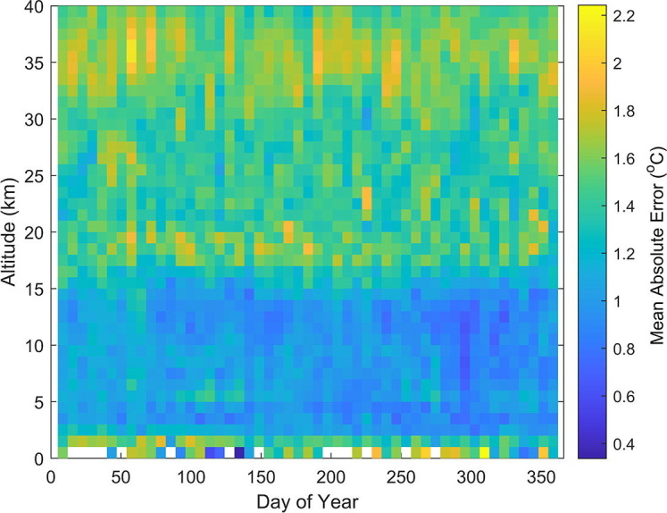
Seasonal variation of the Mean Absolute Error computed as a function of altitude, using the test dataset.
4. Conclusion
A new artificial intelligence based method was used to investigate the effect of the April to September 2020 lockdown on 3-dimensional atmospheric temperatures in Nigeria, equatorial Africa. Artificial neural networks were used to learn trends/patterns in 3-dimensional COSMIC temperature measurements, and subsequently, the trained neural networks are used to predict the expected temperature values for April to September 2020, should there have been no lockdown. The effect of lockdown is deciphered by comparing the neural network predictions with actual COSMIC measurements during the lockdown.
In overall, the results reveal that the mean altitudinal (0 to 40 km) temperatures rose by about 1.1 °C above the expected value during the lockdown. The observed increase in mean altitudinal atmospheric temperatures was linked to decrease in aerosols and precursor emissions during the enforced lockdown, which gave rise to a net decrease in absorption of radiation entering the Earth.
Further analysis at 1 km resolution reveals that the temperature increments were less than 0.5 °C at most of the altitudes, and slightly greater than 1 °C at altitudes of 28 and 29 km. Particularly, two peaks of temperature increments were observed at altitudes of 28 km and 5 km. These altitudes are observed to be similar to those in which maximum concentrations of ozone (in the stratospheric and tropospheric ozone layers) have been detected in the region of the present study.
The temperatures were also observed to drop below expected values at altitudes close to the Earth surface (0–2 km), and at altitudes of 17–20 km (which correspond to the tropopause/lower altitudes of the stratosphere). Atmospheric cooling at altitudes close to the ground was explained to be as a result of reduction in anthropogenic heat fluxes due to the enforced lockdown. Cooling at the lower stratospheric altitudes was suggested to be connected with atmospheric constituent circulations across the troposphere-stratosphere boundary.
There was also an investigation into the significance of the solar activeness (represented by sunspot number) as an input for the neural network training. The results show that including the sunspot number as input for the training did not improve prediction accuracy of the networks, indicating that the solar activity does not play a significant role in deciding the atmospheric temperatures.
Declaration of Competing Interest
The authors declare that they have no known competing financial interests or personal relationships that could have appeared to influence the work reported in this paper.
Acknowledgments
Acknowledgement
We are grateful to the COSMIC team for making atmospheric temperature data from the Constellation Observing System for Meteorology, Ionosphere, and Climate available at https://data.cosmic.ucar.edu/gnss-ro/. We thank the OMNIWeb (https://omniweb.gsfc.nasa.gov/form/dx1.html) for making sunspot number data used in this work available. The second author (Loretta Onuorah) is grateful to the Centre for Atmospheric Research for granting her research visit application to the Centre, and for the technical support and provisions they gave in the course of this research.
Handling Editor: M. Santosh
References
- Adhikari L., Ho S.-P., Zhou X. Inverting COSMIC-2 phase data to bending angle and refractivity profiles using the full spectrum inversion method. Remote Sens. 2021;13(9):1793. doi: 10.3390/rs13091793. [DOI] [Google Scholar]
- Ali S.A., Ali S.A., Suhail N. Ozone depletion, a big threat to climate change: What can be done? Global J. Pharm. Pharm. Sci. 2017;1(2):1–5. [Google Scholar]
- Baboo S.S., Shereef K.I. An efficient weather forecasting system using Artificial Neural Network. Intern. J. Env. Sci. Dev. 2010;1(4):321–326. [Google Scholar]
- Chowdhuri, I., Pal, S.C., Arabameri, A., Thao Thi Ngo, P., Roy, P., Saha, A., Ghosh, M., Chakrabortty, R., 2021. Have any effect of COVID-19 lockdown on environmental sustainability? A study from most polluted metropolitan area of India. Stoch. Environ. Res. Risk Assess. https://doi.org/10.1007/s00477-021-02019-8. [DOI] [PMC free article] [PubMed]
- Diederen K.M.J., Schultz W. Scaling prediction errors to reward variability benefits error-driven learning in humans. J. Neurophys. 2015;114(3):1628–1640. doi: 10.1152/jn.00483.2015. [DOI] [PMC free article] [PubMed] [Google Scholar]
- El-Borie M.A., Thabet A.A., El-Mallah E.S., Abd El-Zaher M., Bishara A.A. The response of the atmosphere to solar variations. Indian J. Phys. 2020;94(6):737–752. doi: 10.1007/s12648-019-01502-x. [DOI] [Google Scholar]
- Fadare D.A. Modelling of solar energy potential in Nigeria using an artificial neural network model. App. Energy. 2009;86(9):1410–1422. doi: 10.1016/j.apenergy.2008.12.005. [DOI] [Google Scholar]
- Gettelman, A., Lamboll, R., Bardeen, C.G., Forster, P.M., Watson-Parris, D., 2021. Climate impacts of COVID-19 induced emission changes. Geophys. Res. Lett. 48(3), e2020GL091805. https://doi.org/10.1029/2020GL091805.
- Gil-Alana L.A., Yaya O.S., Shittu O.I. Global temperatures and sunspot numbers. Are they related? Physica A: Stat. Mech. Appl. 2014;396:42–50. [Google Scholar]
- Gore A. Earthscan; London: 1992. Earth in the balance: forging a new common purpose; p. 407. [Google Scholar]
- Guha S., Govil H. COVID-19 lockdown effect on land surface temperature and normalized difference vegetation index. Geomatics, Nat. Hazards Risk. 2021;12(1):1082–1100. doi: 10.1080/19475705.2021.1914197. [DOI] [Google Scholar]
- Herndon J.M., Whiteside M. Geophysical consequences of tropospheric particulate heating: Further evidence that anthropogenic global warming is principally caused by particulate pollution. J. Geo. Env. Earth Sci. Int. 2019:1–23. doi: 10.9734/jgeesi/2019/v22i430157. [DOI] [Google Scholar]
- Hyrkkänen J., Kilpinen J., Nurmi P., Kaurola J., Brockmann M. Error characteristics of temperature forecast in Finland for the period 1979–2011 in relation to various weather patterns. Met. Appl. 2016;23(2):244–253. doi: 10.1002/met.2016.23.issue-210.1002/met.1550. [DOI] [Google Scholar]
- Ibrahim R.L., Ajide K.B., Olatunde Julius O. Easing of lockdown measures in Nigeria: Implications for the healthcare system. Health Policy Technol. 2020;9(4):399–404. doi: 10.1016/j.hlpt.2020.09.004. [DOI] [PMC free article] [PubMed] [Google Scholar]
- Id M., Yun Z., Patrick B. Simulation and Prediction of Land Surface Temperature (LST) Dynamics within Ikom City in Nigeria Using Artificial Neural Network (ANN) J. Rem. Sens. GIS. 2015;05(01) doi: 10.4172/2469-4134.1000158. [DOI] [Google Scholar]
- Javeed S., Alimgeer K.S., Javed W., Atif M., Uddin M., Deng Y. A modified artificial neural network based prediction technique for tropospheric radio refractivity. PLoS ONE. 2018;13(3):e0192069. doi: 10.1371/journal.pone.0192069. [DOI] [PMC free article] [PubMed] [Google Scholar]
- Kenabatho P.K., Parida B.P., Moalafhi D.B., Segosebe T. Analysis of rainfall and large-scale predictors using a stochastic model and artificial neural network for hydrological applications in southern Africa. Hydr. Sci. J. 2015:1–13. doi: 10.1080/02626667.2015.1040021. [DOI] [Google Scholar]
- Kisi O., Uncuoglu E. Comparison of three back-propagation training algorithms for two case studies. Indian J. Eng. Mater. Sci. 2005;12:434–442. [Google Scholar]
- LEGIST Nigeria Extends Phase 3 COVID-19 Lockdown, Keeps Schools Open. 2021. https://placng.org/Legist/nigeria-extends-phase-3-covid-19-lockdown-keeps-schools-open/ Retrieved from.
- Levenberg K. A method for the solution of certain nonlinear problems in least squares. Q. Appl. Math. 1944;2(2):164–168. [Google Scholar]
- Liou Y.-A., Nguyen K.-A., Ho L.-T. Altering urban greenspace patterns and heat stress risk in Hanoi City during Master Plan 2030 implementation. Land Use Pol. 2021;105:105405. doi: 10.1016/j.landusepol.2021.105405. [DOI] [Google Scholar]
- Mandal I., Pal S. COVID-19 pandemic persuaded lockdown effects on environment over stone quarrying and crushing areas. Sci. Tot. Env. 2020;732:139281. doi: 10.1016/j.scitotenv.2020.139281. [DOI] [PMC free article] [PubMed] [Google Scholar]
- Meadows A.J. A hundred years of controversy over sunspots and weather. Nature. 1975;256(5513):95–97. doi: 10.1038/256095a0. [DOI] [Google Scholar]
- Neubauer D., Ferrachat S., Siegenthaler-Le Drian C., Stier P., Partridge D.G., Tegen I., Bey I., Stanelle T., Kokkola H., Lohmann U. The global aerosol–climate model ECHAM6.3–HAM2.3 – Part 2: Cloud evaluation, aerosol radiative forcing, and climate sensitivity. Geosci. Model Dev. 2019;12(8):3609–3639. doi: 10.5194/gmd-12-3609-2019. [DOI] [Google Scholar]
- Nguyen T.H., Liou Y.A., Nguyen A.K., Sharma R.C., Phien T.D., Liou C.-L., Cham D.D. Assessing the effects of land-use types in surface urban heat islands for developing comfortable living in Hanoi City. Rem. Sens. 2018;10(12):1965. [Google Scholar]
- Okoh, D., Habarulema, J.B., Rabiu, B., Seemala, G., Wisdom, J.B., Olwendo, J., Obrou, O., Matamba, T.M., 2020. Storm‐time modeling of the African regional ionospheric total electron content using artificial neural networks. Sp. Weath. 18, e2020SW002525. https://doi.org/10.1029/2020SW002525.
- Okoh, D., Onuorah, L., Rabiu, B., 2021. Neural Network based MATLAB function for Atmospheric Temperature Prediction in Nigeria (Version 1.0). Zenodo. http://doi.org/10.5281/zenodo.4792261.
- Okoh D., Seemala G., Rabiu B., Habarulema J.B., Jin S., Shiokawa K., Otsuka Y., Aggarwal M., Uwamahoro J., Mungufeni P., Segun B., Obafaye A., Ellahony N., Okonkwo C., Tshisaphungo M., Shetti D. A neural network-based ionospheric model over Africa from constellation observing system for meteorology, ionosphere, and climate and ground global positioning system observations. J. Geophys. Res.: Sp. Phys. 2019;124(12):10512–10532. doi: 10.1029/2019JA027065. [DOI] [Google Scholar]
- Okoh D., Yusuf N., Adedoja O., Musa I., Rabiu B. Preliminary results of temperature modelling in Nigeria using neural networks. Am. Meteorol. Soc. Weather. 2015;70(12):336–343. doi: 10.1002/wea.2559. [DOI] [Google Scholar]
- Omilana, T., 2020. Buhari extends phase two of COVID-19 lockdown by four weeks. Retrieved from https://guardian.ng/.
- Oyeyemi, T., 2020. Remarks by The Chairman, PTF on COVID-19 at the national briefing of Monday, June 1, 2020. Ministry of federal information and culture. Retrieved from https://fmic.gov.ng/.
- Pal S., Das P., Mandal I., Sarda R., Mahato S., Nguyen K.-A., Liou Y.-A., Talukdar S., Debanshi S., Saha T.K. Effects of lockdown due to COVID-19 outbreak on air quality and anthropogenic heat in an industrial belt of India. J. Clean. Prod. 2021;297:126674. doi: 10.1016/j.jclepro.2021.126674. [DOI] [PMC free article] [PubMed] [Google Scholar]
- Randel W.J., Polvani L., Wu F., Kinnison D.E., Zou C.-Z., Mears C. Troposphere-stratosphere temperature trends derived from satellite data compared with ensemble simulations from WACCM. J. Geophy. Res.: Atm. 2017;122(18):9651–9667. doi: 10.1002/2017JD027158. [DOI] [Google Scholar]
- Reuters, 2021. COVID-19 TRACKER: Nigeria. Available at https://graphics.reuters.com/world-coronavirus-tracker-and-maps/countries-and-territories/nigeria/. Accessed 22 September 2021.
- Sahani N., Goswami S.K., Saha A. The impact of COVID-19 induced lockdown on the changes of air quality and land surface temperature in Kolkata city, India. Spat. Inf. Res. 2021;29(4):519–534. doi: 10.1007/s41324-020-00372-4. [DOI] [Google Scholar]
- Scafetta, N., 2014. Global temperatures and sunspot numbers. Are they related? Yes, but non linearly. A reply to Gil-Alana et al. (2014). Physica A: Stat. Mech. & Appl. 413, 329–342. doi:10.1016/j.physa.2014.06.047.
- Schemper M. Predictive accuracy and explained variation. Stat. in Med. 2003;22(14):2299–2308. doi: 10.1002/sim.1486. [DOI] [PubMed] [Google Scholar]
- Schwentek H., Elling W. Increase in the response of the Earth's atmosphere to the sunspot cycle with height above sea level. Sol. Phys. 1981;74(2):355–372. doi: 10.1007/BF00154523. [DOI] [Google Scholar]
- Seman, S. (2020). Introductory Meteorology: Assessing Forecast Accuracy. Department of Meteorology and Atmospheric Science, Penn State College of Earth and Mineral Sciences, https://www.e-education.psu.edu/meteo3/node/2285. Accessed 24 June 2021.
- Wilamowski, B.M., Iplikci, S., Kaynak, O., Efe, M.O., 2001. An algorithm for fast convergence in training neural networks, IJCNN'01. International Joint Conference on Neural Networks. Proceedings (Cat. No.01CH37222), vol. 3, pp. 1778-1782. doi: 10.1109/IJCNN.2001.938431.
- WMO, 2010. What is ozone and where is it in the atmosphere? https://csl.noaa.gov/assessments/ozone/2010/twentyquestions/Q1.pdf. Accessed 24 June 2021.
- Worldometers, 2021. COVID-19 Coronavirus Pandemic. Available at: https://www.worldometers.info/coronavirus/. Accessed 13 March 2021.
- Wuebbles, D., 2020. Ozone layer. Encyclopedia Britannica, https://www.britannica.com/science/ozone-layer. Accessed 24 June 2021.
- Xu Z., Zhao L. Accurate and ultra-fast estimation of Brillouin frequency shift for distributed fiber sensors. Sen. Actuat. A: Phys. 2020;303:111822. doi: 10.1016/j.sna.2019.111822. [DOI] [Google Scholar]
- Yu C., Hu D., Wang S., Chen S., Wang Y. Estimation of anthropogenic heat flux and its coupling analysis with urban building characteristics–A case study of typical cities in the Yangtze River Delta. China. Sci. Tot. Environ. 2021;774:145805. doi: 10.1016/j.scitotenv.2021.145805. [DOI] [Google Scholar]
- Zheng Y., Huang L., Zhai J. Divergent trends of urban thermal environmental characteristics in China. J. Clean. Prod. 2021;287:125053. doi: 10.1016/j.jclepro.2020.125053. [DOI] [Google Scholar]