

Abstract
Using a 3D rotational shear wave elasticity imaging (SWEI) setup, 3D shear wave data were acquired in the vastus lateralis of a healthy volunteer. The innate tilt between the transducer face and the muscle fibers results in the excitation of multiple shear wave modes, allowing for more complete characterization of muscle as an elastic, incompressible, transversely isotropic (ITI) material. The ability to measure both the shear vertical (SV) and shear horizontal (SH) wave speed allows for measurement of three independent parameters needed for full ITI material characterization: the longitudinal shear modulus μL, the transverse shear modulus μT, and the tensile anisotropy χE. Herein we develop and validate methodology to estimate these parameters and measure them in vivo, with μL = 5.77 ± 1.00 kPa, μT = 1.93 ± 0.41 kPa (giving shear anisotropy χμ = 2.11 ± 0.92), and χE = 4.67 ± 1.40 in a relaxed vastus lateralis muscle. We also demonstrate that 3D SWEI can be used to more accurately characterize muscle mechanical properties as compared to 2D SWEI.
Keywords: Muscle, Shear Wave Elastography, Transverse Isotropy
I. Introduction
SHEAR wave elasticity imaging (SWEI) and other acoustic radiation force impulse (ARFI) methods have been used to measure mechanical properties in a wide variety of tissues [1]–[3]. ARFI and SWEI methods employ a conventional clinical ultrasound transducer to create a small amplitude (< 50 μm) localized displacement in the tissue, inducing shear waves that spread outward radially from the push location and are tracked by subsequent ultrasound frames [4]. Under the assumption of a linear, isotropic, and elastic material [4]–[6], the shear modulus μ can be calculated from the measured shear wave speed c and tissue density ρ as
| (1) |
Musculoskeletal SWEI is a wide field of research. Studies have indicated differences in shear wave speeds related to sex [7]–[9], age [8], [10], [11], contractile state [12]–[14] and muscle related diseases such as myopathies [15], [16], dystrophies [17], [18], and muscle spasticities [19]–[22]. The existing research shows uncertainty and lack of repeatability among SWEI measurements in skeletal muscle using current tools [23]–[28], which limits clinical adoption. However, the volume of research to date demonstrates an interest by the orthopedic and neurology communities in noninvasively assessing muscle material properties.
Skeletal muscle is commonly modeled as a transversely isotropic (TI) material due to the alignment of muscle fibers along an axis of symmetry, typically oriented along the direction of muscle contraction. A linear, elastic TI material can be characterized by five parameters [29]–[34]. Furthermore, if the material is assumed to be incompressible, these five parameters are reduced to three [29], [30]. In this study we model skeletal muscle as an incompressible TI (ITI) material characterized by three parameters: the longitudinal shear modulus μL, the transverse shear modulus μT, and a single parameter modeling the joint effect of the longitudinal and transverse Young’s moduli EL and ET. In previous work we have reported this third parameter as the ratio ET/EL [29], [30]; herein we report tensile anisotropy χE [35], defined as
| (2) |
This allows for easy comparison to shear anisotropy χμ [35], defined as
| (3) |
Many studies to date have measured the directional dependence of shear wave propagation in muscle, reporting a wide range of speeds along and across the fiber axis [16], [24], [36]–[50]. These reports used an experimental setup similar to that shown in Fig. 1(a), where the fiber symmetry axis is in a plane parallel to the transducer face, allowing for the measurement of shear wave speeds along and across the muscle fiber axis. The shear moduli μL and μT that characterize shear wave propagation along and across the muscle fiber axis can be calculated from these speeds using (1). However tensile anisotropy χE cannot be determined using (1).
Fig. 1.
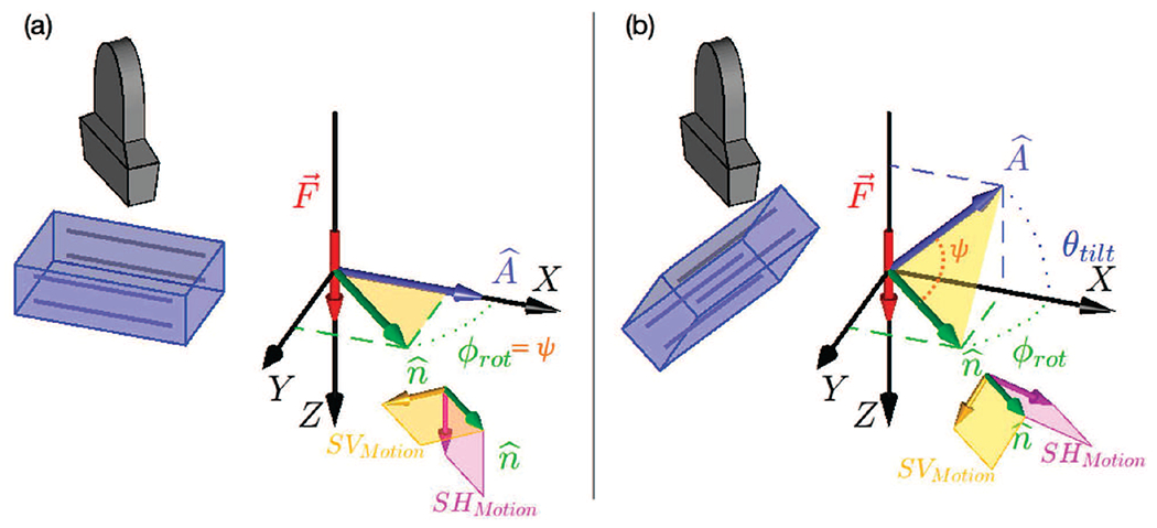
(a) 3D SWEI orientation with ARFI push excitation normal to muscle fiber direction (i.e. muscle symmetry axis, ). represents the direction of wave propagation along which the shear wave speed is computed. ϕrot is the angle between and in the XY plane. In a TI material, two shear wave modes with different polarizations can be excited: the shear horizontal (SH) mode, shown in pink, which is always perpendicular to the plane and the shear vertical (SV) mode, shown in yellow, which is in the plane. With and at normal incidence, as in (a), the SH mode is the primary mode excited in this configuration. (b) 3D SWEI orientation with ARFI push excitation at an angle θtilt away from normal incidence to the muscle symmetry axis (). With a nonzero θtilt both the SH and SV modes are excited and have displacement components in the Z (axial) imaging direction in the material. The angle ψ between A and is shown in orange in (b), while in (a) ψ = ϕrot.
Recently, our group has demonstrated that it is possible to excite and observe multiple shear wave propagation modes in a uniaxially stretched polyvinyl alcohol phantom in which the stretch axis represents the material symmetry axis [51]. This experimental setup is similar to that shown in Fig. 1(b). The key difference compared to the typical setup shown in Fig. 1(a) is that the material symmetry axis is tilted with respect to the ultrasonic acoustic radiation force push beam . With this setup, both the SH and SV propagation modes are excited by an ARFI force directed along the Z axis. Measurement of both the SH and SV wave modes enables characterization not only of μL, μT, and χμ from the SH mode, as measured by a typical setup (Fig. 1(a)), but also of χE, which is dependent upon the SV mode. Herein, we present a method to exploit this geometry and estimate μL, μT, χμ and χE using Green’s function (GF) simulations. We validated our method using finite element method (FEM) simulations, and we also apply this approach to estimate these parameters in in vivo muscle.
II. Background
A. Linear, Elastic, Incompressible, Transversely Isotropic (ITI) Material Models
A linear, elastic material’s stress-strain relationship can be written in terms of a generalized Hooke’s law between the stress tensor σ and strain tensor ϵ as
| (4) |
where cijkl are the elements of the stiffness tensor that characterize the material. For a TI material, rotational and reflective symmetries of the material about its symmetry axis (Fig. 1) reduce the stiffness tensor to five independent quantities [30]–[33]. These five quantities can be expressed in terms of six engineering constants and one constraint: two Young’s moduli EL and ET along the longitudinal (L) and transverse (T) directions, two shear moduli μL and μT, two Poisson’s ratios, νLT and νTT, and the constraint
| (5) |
In SWEI methods, soft tissues are often treated as quasi-incompressible materials with an acoustic wave (compressional) speed of 1540 m/s, and the shear wave propagation is modeled using incompressible material models. For the case of an ITI material, the Poisson’s ratios, νLT and νTT have specific values [29], [30]
| (6) |
and
| (7) |
These relations, plus the constraint in equation (5), imply that shear wave propagation in an ITI material can be described by three independent material parameters. Here, we use the parameters μT, μL, and χE . Note that we have previously used ET/EL [29], [30] which is related to χE by (2).
B. Wave Propagation in ITI Materials
Plane wave propagation in a TI material can be described in terms of three propagation modes: the pressure or compressional mode (P), in which the polarization is aligned with the propagation direction (Fig. 1), and the shear horizontal (SH) and shear vertical (SV) wave modes, in which the polarization is perpendicular to the propagation direction . Particle motion in the SH wave mode is in the plane perpendicular to the plane formed by the material symmetry axis and propagation direction (the pink planes in Fig. 1), while particle motion in the SV wave mode is in the plane (yellow planes in Fig. 1).
In the limit of an ITI material, the phase velocity of the P-wave becomes infinite, and we will ignore this propagation mode. The phase velocities vSH and vSV of the SH and SV modes are given in terms of the angle ψ between and [29], [30] as
| (8) |
and
| (9) |
Equation (8) shows that the SH mode depends only on the observation direction, μL, and μT, but is not affected by the tensile anisotropy, χE. For this mode, the group velocity VSH(ψ) is given by an elliptical shape [30], [32], [34], [52] as
| (10) |
The group velocity for the SV propagation mode does not reduce to a simple expression like (10) as the SV mode can support multiple shear wave speeds for a particular propagation direction, depending on the specific material parameters considered (see Fig. 1 of Rouze et al. [29]). However, we have recently reported tractable calculations using Green’s functions that describe both the SV and SH modes in an elastic, ITI material, which we employ herein to characterize χE [30].
C. Practical Implementation in Ultrasound
In each of the two configurations seen in Fig. 1, the transducer rotates around its central axis. As such, each 2D imaging frame contains the axial imaging dimension Z, perpendicular to the transducer face, and a lateral (radial) dimension, parallel to the transducer face, corresponding to in Fig. 1 as determined by the rotational angle ϕrot of the transducer.
SWEI methods preferentially push and track material displacements in the axial (Z) dimension. As such, when the excitation from the transducer is normal to the fiber direction (Fig. 1(a), ), we only track the SH mode of propagation. In this configuration, the SV mode does not have an appreciable component in the Z (axial imaging) direction, and thus would not be detected with our experimental setup. However when the fiber direction is tilted relative to the transducer face, as seen in Fig. 1(b), the planes containing the SV mode and SH modes are tilted such that both modes have components in the Z dimension, and thus can be excited and monitored with our experimental setup. In both Figs. 1(a) and (b) the transducer rotates around its axis to allow us to measure the shear wave propagation in 3D (see Supplemental Animation 1). Similarly, the tilt angle θtilt between the fibers and the lateral imaging axis at each propagation direction can change depending on the probe positioning (ϕrot) and muscle architecture because different muscles have different fiber orientations relative to the skin surface. This affects the magnitude of the tissue displacement in the axial imaging orientation (Z) for both the SV and SH modes (see Supplemental Animation 2).
Typically, experiments using 2D SWEI determine μL and μT from measurements of the group shear wave speed (SWS) along and across the muscle fibers using the configuration shown in Fig. 1(a). Because the tensile anisotropy χE appears only in the equation describing the SV wave mode (9), it is necessary to measure both the SV and SH waves to fully characterize an ITI material. This is achieved herein by leveraging the tilted fiber geometry inherent to the vastus lateralis during in vivo imaging.
III. Methods
A. Experimental Acquisitions in in vivo Muscle
A volumetric rotational 3D-SWEI acquisition system was obtained using a rotating linear array probe [53]. A Philips ATL L7-4 array (Philips®, Andover, MA) was attached to a Verasonics Vantage 256 (Verasonics®, Kirkland, WA) ultrasound system. The transducer was mounted in a custom holder attached to a rotation stage (XPS-Q8, Newport®, Irvine, CA) to allow rotation about the transducer’s vertical axis.
A healthy, 53 year old female volunteer with no known muscular diseases or injuries was selected and written informed consent was obtained for participation in a Duke University Institutional Review Board-approved study. The subject was placed in a lateral position with a rolled towel between the knees. A water bath with Tegaderm bottom was used to ensure a consistent water path between the transducer and the muscle throughout the full rotation of the probe. Ultrasound gel was applied between the leg and the Tegaderm box, and any air bubbles were manually removed by smoothing the Tegaderm face against the leg. The water bath and transducer were positioned so the center of rotation was in the main body of the vastus lateralis muscle, approximately halfway between the upper trochanter and the quadriceps tendon (Fig. 2a).
Fig. 2.
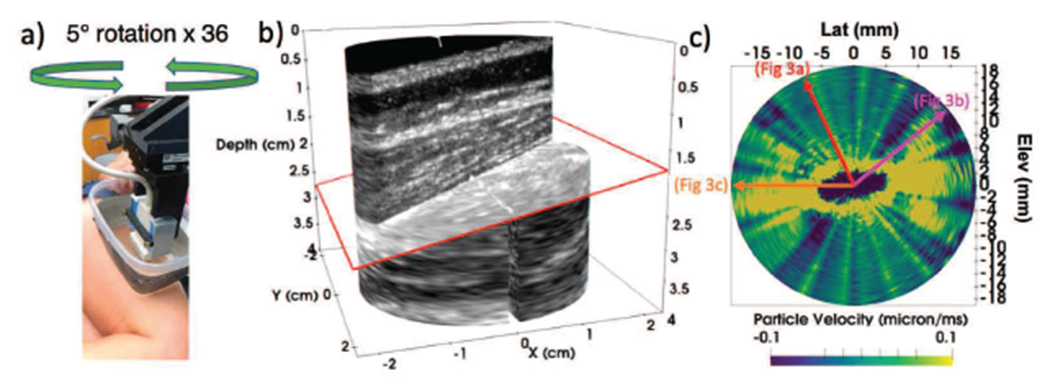
Data acquisition setup. Fig. a shows an L7-4 transducer placed in the rotation stage set up, Tegaderm box with gel against the vastus lateralis muscle, to be rotated in 5 degree steps. Fig. b shows an example B-mode image obtained from one of the rotational imaging planes (ϕrot = 15°) The red arrow shows the axial depth of the SWEI push focus. The yellow lines are approximations of the proximal and distal vastus lateralis aponeuroses
Thirty-six frames were acquired in 5 degree rotation (ϕfiber) increments with a total of 3 seconds between each frame, including time for the transducer to rotate. As each frame included a left moving and right moving wave, the transducer only had to be rotated 180 degrees to acquire a full 360 degree volume. The sequence for each rotation position consisted of a 4 MHz push focused at 20 mm axially, centered under the transducer laterally, followed by a repeating pattern of 5.2 MHz tracking plane waves at 10 kHz pulse repetition frequency angled at −3°, 0°, and 3° consecutively for ~ 40 ms. The tracking planes were coherently compounded with a rolling window so that each resulting track plane included one of the three original angles as seen in Table I, while still allowing for full temporal sampling.
TABLE I.
Coherently Compounded Track Configuration
| Sub-Frame 1 | −3° | → | 0° | → | 3° |
| Sub-Frame 2 | 0° | → | 3° | → | −3° |
| Sub-Frame 3 | 3° | → | −3° | → | 0° |
For each track pulse, a 4x4 cm (axial x lateral imaging plane) region of interest was reconstructed with a pixel resolution of 400 μm axially and 200 μm laterally. This process of acquiring a full 360 degree rotation acquisition (36 frames) was performed a total of 4 times on two different days in the same subject.
Within each rotational plane, axial displacements were calculated using Kasai’s algorithm with a 1.5λ kernel [?] and separated into the left and right moving shear waves. The displacement data were temporally low pass filtered at 600 Hz, and differentiated into particle velocity data. The transverse plane (X-Y imaging plane in Fig. 1) was extracted for further analysis by averaging over a 1 mm depth axially centered around the push focal depth of 20 mm. A sample B-mode image is shown in Fig. 2b for rotation position ϕrot = 15° and shows the tilted fiber orientation in the lateralis muscle. The fiber tilt angle θtilt was determined by 2DFT of the B-mode image, as described in Section III-C.
B. Shear Wave Speed Estimation
Shear wave speeds were calculated for each space time trajectory using the Radon sum algorithm [56]. Typically, a lateral range of 6 to 16 mm was used in the estimate, however, this range was adjusted for each space-time trajectory based on the range over which a distinct trajectory could be visually identified. The white lines overlaid on the space time signals in Fig. 3 show the lateral range used in the speed estimate. If a single wave mode was present, it was assumed to be SH mode, if two trajectories were present, the faster was assumed to be the SV mode. For cases with two shear wave trajectories, such as Fig. 3b, individual speeds were estimated by masking the Radon sum images (see Fig. 2 of Rouze et al. 2010 [56]) to identify the trajectory for each propagation mode. All trajectories were verified visually by a single reader.
Fig. 3.
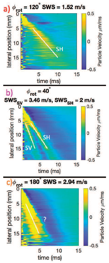
Example space time plots from experimental acquisitions. The top row (Fig. a) shows an example space time plot of a transducer angle (ϕrot = 120°) where there is only one trajectory and one wave mode present, which is the SH mode. Fig. b shows an example of an angle (40°) from the same acquisition as Fig. a where there are two shear wave speeds clearly present on the space time plot. The faster wave is the SV mode (3.49 m/s) and the slower the SH mode (2 m/s). The bottom row, Fig. c, shows an example of an angle (180°) from the same overall acquisition as Fig. a and Fig. b where the SV mode and the SH mode waves are merged. Although a speed is identified on this image, visual assessment indicates that it is neither the SV nor the SH trajectory, and thus the speed estimate is excluded from the SH mode ellipse fitting. All of these data in Fig. a, b, and c, are also shown in Fig. 6
For some trajectories, such as Fig. 3,c it was not possible to assign the estimated speed to either the SH or SV mode as the waves appeared merged. In these cases, no speeds were recorded and these propagation directions were omitted from further analysis.
C. Iterative Parameter Estimation of θtilt, ϕfiber, μL, and μT
A flowchart explaining the full algorithm workflow is provided for reader convenience in Fig. 4. The values of the full acquisition’s overall rotation angle ϕfiber) and tilt (θtilt) and the values of μL and μT can be estimated using a three step procedure as follows.
Fig. 4.
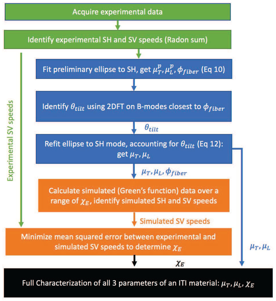
Flowchart of data processing steps. The green boxes show acquiring and initial processing of the experimental data (Sections III-A and III-B). The blue steps show the steps for determining θtilt, ϕrot, μL, and μT from Section III-C. The orange boxes show the iterative parameter fitting steps that use the simulated Green’s function data to determine ET/EL (Section III-D.)
First, preliminary estimates, as indicated by superscript p of , , and can be found by assuming an elliptical shape based on (10).
| (11) |
where .
Nonlinear least square fitting was used to estimate , , and by minimizing the sum of the squares difference between the measured SH speeds, and the predicted speeds from (11).
Second, the estimated fiber rotation was used to determine the fiber tilt angle θtilt by examining the B-mode images for the transducer rotation nearest to . These B-mode images were analyzed using a two dimensional Fourier transform (2DFT) approach as seen in Fig. 5. We assumed that the fibers were represented by a series of parallel lines at a given tilt. In order to efficiently calculate this tilt, we took the 2DFT of the B-mode image over a region of interest and integrated radially within the 2DFT plane. The angle of peak signal was related to the B-mode tilt using the rotation property of 2DFT as seen in Fig. 5(b).
Fig. 5.
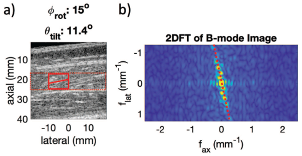
Fig. a shows an example B-modes for determining θtilt. The red box show sample 2DFT regions and resultant θtilt estimate on the B-mode. This tilt, θtilt, is then used to re-fit the SH mode ellipse with a geometric scale factor to account for θtilt using (12). Fig. b shows the 2D FFT of the selected region from Fig. a. The dotted red line shows the peak intensity representing the tilt of the fibers, θtilt, in this case 11°
Finally estimates of μL, μT, and ϕfiber were determined by repeating the the fitting procedure (11), but with the angle ψ determined relative to the material symmetry axis,
| (12) |
D. Estimate of in vivo ET/EL Using Simulated Shear Wave Signals
The third parameter, ET/EL, needed to fully characterize an incompressible, elastic TI material was determined by simulating shear wave signals using a range of values for ET/EL and comparing the shear wave speeds from these simulations to the measured in vivo SV mode speeds. The shear wave signals were calculated using Green’s function techniques as described by Rouze et al. [30], using the ARFI excitation force calculated using Field II [57] modeling our experimental setup.
The final value of ET/EL was estimated by calculating a series of XY plane simulated shear wave signals for a range of values of ET/EL and selecting the value which minimized the sum of the squared differences between the simulated and experimentally measured SV speeds.
| (13) |
where n is the number of detected experimental SV speeds present. This mean squared error was calculated for each Green’s function plane (13) and an error minimization was performed using quadratic fitting to find the Green’s function most similar to the experimental data.
IV. Results
As the transducer rotates, as shown in Fig. 2, shear waves trajectories, such as those seen in Fig. 3, are seen at each rotation angle in the lateral and axial dimensions. Fig. 6 shows particle velocity shear wave signals from a single acquisition in an in vivo vastus lateralis muscle as a function of space and time for 18 transducer rotation angles spaced at 10° rotation steps. As the transducer only rotates around 180°, at each rotation angle the left moving propagation direction and right moving propagation direction signals are separated, giving two signals per acquisition (36 signals shown in Fig. 6 obtained from 18 transducer rotation angles). This set represents one half of the signals acquired in a complete data set with 5° rotation steps.
Fig. 6.
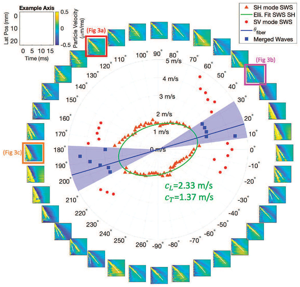
Space time plots and speeds at many angles. The subplots going around the ring show space-time plots in 10° increments of ϕrot (transducer rotation). An example axis label for each subplot is shown in the upper left. The white lines on each subplot identify the trajectory of speeds identified. Each space time plot contains 0, 1, or 2 trajectories. The number of waves identified and calculated speeds are seen in the inner circle plot. The slower SH mode wave speeds are seen in orange triangles, while the faster SV speeds are in red circles. The ellipse fit to the SH speeds is shown in green (using (11) and (12)), as is the speeds along the major axis of the ellipse (cparallel), and the minor axis of the ellipse (cperpendicular). The blue line shows the rotational angle of the fibers ϕfiber corresponding to the major axis of the ellipse. These values of cparallel and cperpendicular are after θtilt has been accounted for (see Section III-C.)
A key observation in Fig. 6 is that, as the transducer rotational position is varied, multiple shear wave signals are observed for rotational directions near ϕrot = −10°, 30°, 170° and 210°, while only a single shear wave signal is observed for rotational angles near ϕrot = −90° and 90°.
To see the difference between multiple trajectories better, enlarged space-time images of selected shear wave signals are shown in Fig. 3, corresponding to ϕrot = 120°, 40°, and 180°. Because the fiber tilt shown in Fig. 2b is small, it is expected that the largest amplitude signal is the SH propagation mode. When a second shear wave signal is seen, for example in Fig. 3b, this mode is identified as the SV propagation mode.
In the center of Fig. 6 the shear wave speeds are plotted as a function of propagation angle with the SH propagation mode shown as orange triangles, and the SV propagation mode shown in red circles. For propagation directions near ϕrot = 15° and 195° the SH and SV trajectories on the space-time images appear to merge, and it was not possible to assign an estimated speed to either mode. These cases were omitted from further analysis.
From the B-mode image shown in Fig. 2b and the distributions of shear wave speeds for the SH propagation mode shown in the center of Fig. 6, it is clear that the material symmetry axis in Fig. 1b is not aligned with the X-axis (0° → 180°) for this example acquisition. Instead this axis is rotated by angle ϕfiber about the Z-axis and is also tilted by an angle of θtilt relative to the X-Y imaging plane.
Following along with the example acquisition shown in Fig. 6, the nonlinear least squares fitting found the preliminary estimates of , resulting in , , and . Note that these are not the values given in Fig. 6 as they are preliminary estimates. For this same acquisition, the 2DFT derived θtilt value from the ϕrot = 15° and 20° were weighted by the results according to the proximity to ϕfiber, with the result for the case shown in Fig. 6 of θtilt = 11° ± 2.5°. Once θtilt was accounted for geometrically, the final values of cparallel = 2.33 m/s, Cperpendicular = 1.37 m/s, meaning μL = 5.41 kPa, μT = 1.89 kPa, and ϕfiber = 11° were found. These results are indicated on Fig. 6.
The top row of Fig. 7 shows sample simulated shear wave particle velocity signals at a time of 3 ms calculated using the angles θtilt and ϕfiber and the material properties μL = 5.41 kPa and μT = 1.89 kPa estimated by our algorithms for three cases ET/EL = 0.199, 0.148, and 0.127. The middle row of Fig. 7 shows corresponding shear wave speeds. An important observation for the simulated signals is that the signal amplitude varies with propagation direction, particularly for the SV propagation mode. Even with the same underlying μL, μT, and ϕfiber, small changes in ET/EL affect the intensity of the SV wave.
Fig. 7.
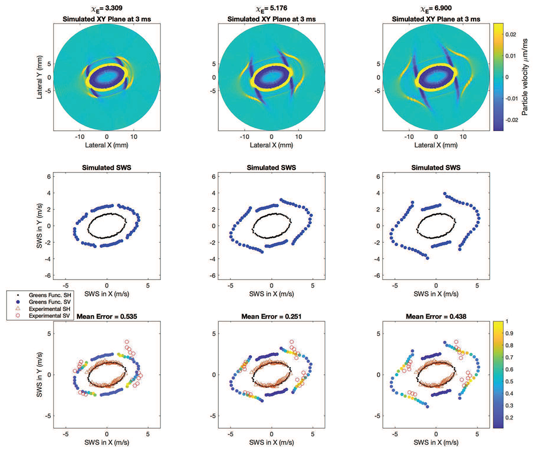
Comparison of Simulated and Experimental Signals. The top row shows the simulated Green’s function signals in the XY plane at 3 ms at three different values of ET/EL. In the middle row and bottom row, the simulated SH (black dots) and SV speeds (blue dots) at each angle are shown. In the bottom row the experimental SH mode is shown in the open orange triangles, and the experimental SV mode is shown in open red circles. In the bottom row the color of the circles show the SV mode strength relative to the other SV mode speeds present (similar to the top row), as calculated by normalizing each by the maximum Radon sum value found across all SV mode speeds in a given Green’s function plane. Yellow indicates a strong SV mode relative to blue. The fact that most of the high amplitude signals (yellow dots) are concordant with the experimental data adds confidence to the biofidelity of this ET/EL estimation approach.
The bottom row of Fig. 7 shows the shear wave speeds from experimental data (Fig. 6) overlaid on the calculated speeds from the middle row. The simulated SV speeds are color coded by the amplitude of the shear wave signal in the top row. We observe that the speeds determined from the signals with the largest shear wave amplitude occur at transducer angles of roughly ϕrot = −10°, 40°, 170° and 220°, which are roughly the same directions where two shear wave signals, both SH and SV, are observed experimentally. The iterative parameter estimation technique using Green’s Functions gave ET/EL = 0.151 for the acquisition shown in Fig. 6. The fact that most of the large amplitude signals in the simulated data are concordant with the experimental data adds confidence to the biofidelity of this ET/EL estimation approach.
In four acquisitions on two different days in the same healthy volunteer, four estimates of μL, μT, and ET/EL were calculated as seen in Fig. 8. Mean and standard deviation values for μL, μT, ET/EL and mean squared error are given in Table II.
Fig. 8.
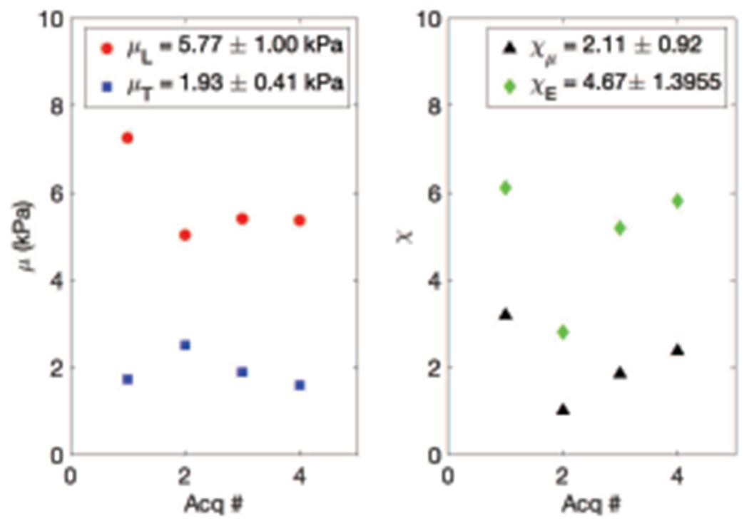
μL, μT, and ET/EL from four acquisitions. On the left, in red circles, μL in kPa, and in blue squares μT in kPa, both vs acquisition number. On the right, in black triangles ET/EL vs acquisition number. Note that ET/EL is limited from 0 to 0.5 so as to highlight the variability in the measurements.
TABLE II.
Mean and Standard Deviation Across 4 Acquisitions
| μL | 5.77 ± 1.00 kPa |
| μT | 1.93 ± 0.41 kPa |
| ET/EL | 0.151 ± 0.051 |
| MSE | 0.244 ± 0.10 (m/s)2 |
Fig. 9 shows for each acquisition the value of the ratio of the two shear moduli μT/μL plotted vs the ratio of the Young’s moduli ET/EL. The blue line represents ET/EL = μT/μL which would be the case for an isotropic material.
Fig. 9.
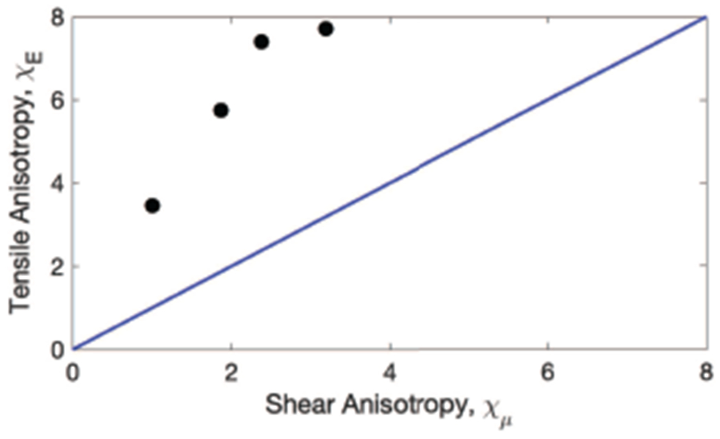
Experimental values of the ratio of shear moduli μT/μL (0.345 ± 0.111) vs ratio of Young’s moduli ET/EL (0.151 ± 0.051). Each experimental acquisition is plotted in black circles. The blue line represents where μT/μL = ET/EL.
Fig. 10 portrays the effect of variability in the 2DFT estimate of B-mode tilt (ϕtilt) on the resultant ET/EL found via the simulated shear wave signal method (III-D). The ϕtilt = 8.5° case represents one standard deviation in tilt below the mean, and ϕtilt = 13.5° represents one standard deviation greater in tilt as estimated on the 2DFT. The percent variability in μL = 6.5%, the percent variability in μT = 0.0%, and the percent variability in ET/EL = 11.3%
Fig. 10.
Effect of variation in θtilt on ET/EL. μL, μT, and ET/EL from the same acquisition at 3 different assumed θtilt values: 8.5°, 11°, 13.5°. On the left in red circles, μL in kPa and μT in blue squares, both vs tilt angle θtilt) in degrees. On the right, in black triangles ET/EL vs θtilt. Note that ET/EL is limited from 0.1 to 0.2 as compared to Fig. 8 so as to highlight the variability in the measurements. The percent variability in μL = 6.5%, the percent variability in μT = 0%, and the percent variability in ET/EL = 11.3%
V. Discussion
In this paper, we demonstrate that measuring both the SV and SH wave modes is possible using 3D SWEI in in vivo muscle by leveraging the tilted geometry of the muscle fibers relative to the transducer face. We also present a method of estimating the tensile anisotropy χE of muscle.
Fig. 7, bottom middle panel, demonstrates the agreement between the GF predicted SV and SH speeds and the in vivo experimental measurements. In the middle column, not only is the error between the GF and the experimental speeds minimized, but the location of the largest amplitude simulated SV signals (yellow and green dots) align with the angles where the experimental SV speeds were observed. The appearance of SV waves experimentally at the four regions where the GF predict the largest amplitude SV waves increases confidence that SV waves are not reflected waves.
As seen in Fig. 8, in each of four acquisitions on two days in the same healthy volunteer, the μL value measured was greater than μT. Additionally, the tensile anisotropy χE was greater than the shear anisotropy χμ in each acquisition.
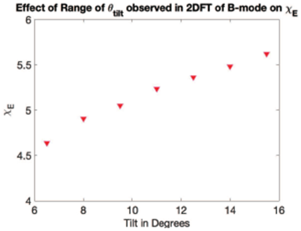
As seen in Fig. 9, as the tilt angle θtilt increases, the calculated χE value also increases monotonically, indicating expected bias if the tilt angle is not correctly computed. However, across a 95% confidence interval of the θtilt = 11.4 ± 2.5° measured in the B-mode data, the variation of χE (0.344) represents only a 6% bias.
To quantify the expected accuracy of our Green’s function approach to estimating χE, for one acquisition, FEM simulations were computed to match the experimental setup with known inputs. As seen in Fig. 10, the matched GF and FEM simulated speeds at angles where there were experimentally observed SV waves varied from each other by only 0.11±0.13 m/s, while the SH wave speeds differences between the GF and FEM were 0.07 ± 0.07 m/s. Additionally, using the Green’s function reconstruction algorithm for this data set found an estimate of χE = 5.30, while the ground truth value was χE = 5.25, meaning a difference of 1%. Using a computational cluster, the GF plane calculations of Z direction displacement and resultant SWS in the XY plane necessary to estimate 120 possible χE values for a given θtilt, μL, and μT took approximately 150 CPU-hours on an Intel®Xeon Gold 3 GHz CPU. We are exploring methods to pre-populate look up tables to reduce this time, but this work is outside the scope of this paper.
The relationship between shear modulus and Young’s modulus in an isotropic, elastic, incompressible material is E = 3μ. However in ITI materials, there is no simple proportional relationship between E and μ in any given direction. As seen in Fig. 8, and as predicted by the equations modeling ITI materials (2)-(3), (5)-(7), χE is not equal to χμ and thus represents an additional independent parameter that may be explored for muscle health characterization.
One of the advantages of a rotational 3D approach is that since all rotational angles are captured in 5° increments, the 3D SWEI methodology presented herein is completely agnostic to the starting position of the fiber rotation ϕfiber relative to the transducer. This means the 3D SWEI approach can be used without first identifying muscle fiber orientation with freehand B-mode imaging.
The values for the shear modulus along the fibers (μL = 5.77 ± 1.00 kPa) are similar but slightly higher than those found by other studies in the vastus lateralis using 2D SWEI (4.5 ± 1.0 kPa [28], 3.6 ± 0.45 kPa [7], 3.3 ± 0.4 kPa [58], and 5.1±1.3 kPa [59]). The use of 3D data herein ensures the μL and μT measurements account for both the rotation ϕfiber and tilt θtilt angles of the muscle fibers. Misalignment in either dimension would result in an underestimation of μL, which could be a source of bias in the results of 2D SWEI studies. In particular, accounting for the tilt angle θtilt in (12) increases our estimates. On average μL increased by 7.6% ± 3.5% when θtilt was incorporated, as compared to the assumption θtilt = 0°.
As seen in the center of Fig. 6, the speeds closest to the major axis of the SH mode ellipse were not included in the ellipse fitting. At those locations, visual assessment of the space-time plots made it clear that the SV and SH modes were spatially overlapping with each other. While the Radon sum algorithm was able to identify a trajectory, visual assessment could not determine if the trajectory was calculated using only SV mode data, only SH mode data, or a combination of both SV and SH mode, so the speed was excluded from further analysis. Supporting this, as seen in Fig. 7 bottom row, directly along the major axis of the ellipse, the SV speed predicted by simulation is very low amplitude compared to other SV speeds at other angles. When the inherent noise of experimental motion tracking is combined with this effect, it is unsurprising that it is difficult to separate the SH and SV modes for these propagation directions in experimental data.
The difficulty in separating the SH and SV waves along the main fiber axis could also be one of many factors contributing to the wide variability in speeds found using 2D SWEI techniques [24]. If the method used to identify the shear wave speed along the fibers does not account for the presence of both SV and SH mode speeds, it is unknown whether the speed measured along the fiber axis is from the SH mode or the SV mode, increasing variability in the measurements. The blue squares and highlighted area of Fig. 6 indicate what speed would be estimated by 2D SWEI if the delineation of SH and SV waves was not considered. Our work overcomes this by informing the estimate of μL with speeds around the ellipse rather than relying solely on speeds aligned with the fiber dimension, and inspecting space-time plots for multiple wave fronts.
As a proof of concept work, this paper presents measurements from only one healthy volunteer. However, the repeatability across multiple days and multiple acquisitions supports the feasibility of this method and motivates the development of 3D SWEI for muscle imaging and measuring mechanical properties of muscle.
The concordance between the Green’s function simulations and in vivo muscle data demonstrate that the linear, elastic, ITI model is a reasonable model in the vastus lateralis of a healthy volunteer. The ability to extend this model to other muscles is limited by the size of the muscle, as when the thickness of the muscle body approaches the shear wavelength it is likely that other wave guiding behavior and boundary effects would influence waves measured. Additionally, a limitation of this method is the requirement that the experimental and simulated parameters are exactly matched, as any mismatches would be expected to introduce bias in the χE estimates.
A notable limitation of this work is that it neglects viscosity. Viscosity introduces dispersion and attenuation in shear wave elastography data, which has been shown to bias estimated parameters based upon group speeds [60]. We have observed some dispersion in vastus lateralis data, primarily across the fibers with less dispersion along the fibers [61], which is consistent with reports from the literature [45]. Thus, it is possible that the SV mode analysis presented here has some bias, which might be addressed at the expense of computational complexity, but is outside the scope of this initial demonstration.
For years, three parameter models of ITI materials have been proposed for muscle SWEI modeling [29], [30], [46], but to date quantification of all three parameters has not been realized in in vivo ultrasound SWEI. Recent demonstration of the ability to resolve two wave fronts in phantoms [51] showed the feasibility of using a tilted excitation to reconstruct tensile anisotropy.
Additionally, Li et al. have investigated these phenomena in biceps brachii and gastrocnemius muscles using 2D SWEI and measurements at 3 specified orientations of the transducer, assuming that the group shear wave speed measured with the transducer at θtilt = 45° represents the SV mode [62]. They found values that result in a χμ of 1.53 in the biceps brachii and 0.31 in the gastrocnemius, and χE of 0.75 in the biceps brachii and 0.81 in the gastrocnemius. All of these values are about 4 times lower than the range of values reported for the vastus lateralis herein. However they also measured a mean vSV of 1.8 m/s, while we found a mean vSV of 3.8 m/s, and given the relationship between and χE seen in (9), it is unsurprising that approximately doubling the SV speed leads to a quadrupling of χE, showing again the importance of accurately measuring the SV speed. The 3D SWEI method herein leverages the tilt concepts but also facilitates characterization in muscles with a range of interrogation angles and fiber orientations.
Three ITI material parameters have been measured in vivo by magnetic resonance elastography (MRE) [48], and in ex vivo animal tissue [49], [50]. Looking at the three muscles in the calf using MRE in vivo, Guo et al. [48] found lower χμ values (soleus 0.50, gastrocnemius 0.80, tibialis anterior 0.27) compared to χμ = 2.11 herein for vastus lateralis, and also χμ values lower than herein (soleus 1.47, gastrocnemius 2.26, tibialis 2.00, compared to χE = 4.67 for vastus lateralis). These lower values for both tensile and shear anisotropy indicate the muscles appeared more isotropic using MRE than with 3D SWEI. It is encouraging that χμ > χμ with both MRE and 3D SWEI. There are several factors that could account for differences between these results. The interrogated muscles reported are different. The nature of the external continuous wave vibration and inversion of the wave equation employed by MRE means the parameters reconstructed are not as localized within the muscle, whereas 3D rotational SWEI measurements of muscle apply to a smaller region of interest (4 cm2). Additionally, the frequency content of MRE in the cited studies (40 Hz, 50 Hz, and 60 Hz in Guo et al.) is lower than the frequency content of SWEI used here (100-400 Hz). As frequency increases shear dissipative effects increase. Thus, there is an expectation that moduli estimated based on an elastic assumption will have an increasing bias as frequency increases. For example, see Yasar et al. [63], which shows that typically both the shear storage and loss moduli monotonically increase with excitation frequency.
The ability to measure tensile anisotropy χE and χμ may provide a unique biomarker for muscle characterization. However, the relationship between these material parameters, as well as μL and μT, and muscle health remains an open question. While still only a proof of concept, determining these relationships has potential application in characterizing a wide variety of muscle diseases including myopathies, dystrophies, muscle spasticities, muscle atrophy, age related sarcopenia, and athletic injury repair and healing.
VI. Conclusion
In this study, we describe measurements of multiple shear wave propagation modes in in vivo muscle using a 3D SWEI experimental setup with a tilted material symmetry axis, shown in Fig. 1(b). Results are reported from measurements made in a healthy volunteer on two different days in the relaxed vastus lateralis muscle, where the fibers are naturally tilted with respect to the skin surface. We demonstrate 3D SWEI can improve estimation of μL and μT by accounting for the effects of fiber rotation ϕfiber and tilt θtilt when evaluating SH mode speeds, which is not possible in 2D SWEI. We also demonstrate 3D SWEI measurement of the SV propagation mode which, when combined with matched Green’s function simulations, allows for estimation of tensile anisotropy, χE.
Supplementary Material
Acknowledgments
The authors would like to thank the funding sources: NIH grant R01CA142824, R01EB022106, and the Duke MEDx Pilot Project Grant.
Footnotes
K. Nightingale, N. Rouze and M. Palmeri hold intellectual property related to acoustic radiation force impulse and shear wave elasticity imaging.
Contributor Information
Anna E. Knight, Department of Biomedical Engineering, Duke University, Durham, NC, 27707 USA.
Courtney A. Trutna, Department of Biomedical Engineering, Duke University, Durham, NC, 27707 USA.
Ned C. Rouze, Department of Biomedical Engineering, Duke University, Durham, NC, 27707 USA.
Lisa D. Hobson-Webb, Duke Department of Neurology, Duke University Health System, Durham, NC, 27707, USA
Annette Caenen, Ghent University, Department of Electronics and Information Systems, IBiTech-bioMMeda Lab Ghent, BELGIUM; Cardiovascular Sciences Department, Cardiovascular Imaging and Dynamics Lab at KU Leuven, Leuven, BELGIUM.
Felix Q. Jin, Department of Biomedical Engineering, Duke University, Durham, NC, 27707 USA.
Mark L. Palmeri, Department of Biomedical Engineering, Duke University, Durham, NC, 27707 USA.
Kathryn R. Nightingale, Department of Biomedical Engineering, Duke University, Durham, NC, 27707 USA.
References
- [1].Sarvazyan A, Hall TJ, Urban MW, Fatemi M, Aglyamov SR, and Garra BS, “an Overview of Elastography – an Emerging Branch of Medical Imaging,” Current medical imaging reviews, vol. 7, no. 4, pp. 255–282, 2011. [DOI] [PMC free article] [PubMed] [Google Scholar]
- [2].Doherty JR, Trahey GE, Nightingale KR, and Palmeri ML, “Acoustic Radiation Force Elasticity Imaging in Diagnostic Ultrasound,” IEEE Transactions on Ultrasonics, Ferroelectrics and Frequency Control, vol. 60, no. 4, 2013. [DOI] [PMC free article] [PubMed] [Google Scholar]
- [3].Sigrist RM, Liau J, Kaffas AE, Chammas MC, and Willmann JK, “Ultrasound elastography: Review of techniques and clinical applications,” Theranostics, vol. 7, no. 5, pp. 1303–1329, 2017. [DOI] [PMC free article] [PubMed] [Google Scholar]
- [4].Sarvazyan AP et al. “Shear Wave Elasticity Imaging: A New Ultrasonic Technology of Medical Diagnostics,” Ultrasound Med. Biol, vol. 24, no. 9, pp. 1419–1435, 1998. [DOI] [PubMed] [Google Scholar]
- [5].Palmeri ML and Nightingale KR, “Acoustic radiation force-based elasticity imaging methods,” Interface Focus, vol. 1, pp. 553–564, 2011. [DOI] [PMC free article] [PubMed] [Google Scholar]
- [6].Shiina T et al. “WFUMB guidelines and recommendations for clinical use of ultrasound elastography: Part 1: Basic principles and terminology,” Ultrasound in Medicine and Biology, vol. 41, no. 5, pp. 1126–1147, 2015. [DOI] [PubMed] [Google Scholar]
- [7].Zhang C and others., “Diagnostic Value of Virtual Touch Tissue Imaging Quantification for Evaluating Median Nerve Stiffness in Carpal Tunnel Syndrome,” Journal of Ultrasound in Medicine, pp. 1783–1791, 2017. [DOI] [PubMed] [Google Scholar]
- [8].Eby SF et al. “Shear wave elastography of passive skeletal muscle stiffness: Influences of sex and age throughout adulthood,” Clinical Biomechanics, vol. 30, no. 1, pp. 22–27, 2015. [DOI] [PMC free article] [PubMed] [Google Scholar]
- [9].Mackintosh S, Young A, Lee A, and Sim J, “Considerations in the application of two dimensional shear wave elastography in muscle,” no. March, pp. 1–9, 2019. [Google Scholar]
- [10].Alfuraih AM, Tan AL, O’Connor P, Emery P, and Wakefield RJ, “The effect of ageing on shear wave elastography muscle stiffness in adults,” Aging Clinical and Experimental Research, vol. 31, no. 12, pp. 1755–1763, 2019. [DOI] [PMC free article] [PubMed] [Google Scholar]
- [11].Lima K. M. M. e., Costa Jύnior JFS, Pereira W. C. d. A., and De Oliveira LF, “Assessment of the mechanical properties of the muscle-tendon unit by supersonic shear wave imaging elastography: A review,” Ultrasonography, vol. 37, no. 1, pp. 3–15, 2018. [DOI] [PMC free article] [PubMed] [Google Scholar]
- [12].Yoshitake Y, Takai Y, Kanehisa H, and Shinohara M, “Muscle shear modulus measured with ultrasound shear-wave elastography across a wide range of contraction intensity,” Muscle and Nerve, vol. 50, no. 1, pp. 103–113, 2014. [DOI] [PubMed] [Google Scholar]
- [13].Shinohara M, Sabra K, Gennisson JL, Fink M, and Tanter ML, “Real-time visualization of muscle stiffness distribution with ultrasound shear wave imaging during muscle contraction,” Muscle and Nerve, vol. 42, no. 3, pp. 438–441, 2010. [DOI] [PubMed] [Google Scholar]
- [14].Chernak LA, Dewall RJ, Lee KS, and Thelen DG, “Length and activation dependent variations in muscle shear wave speed,” Physiological Measurement, vol. 34, no. 6, pp. 713–721, 2013. [DOI] [PMC free article] [PubMed] [Google Scholar]
- [15].Alfuraih AM et al. “Muscle shear wave elastography in idiopathic inflammatory myopathies: a case–control study with MRI correlation,” Skeletal Radiology, vol. 48, no. 8, pp. 1209–1219, 2019. [DOI] [PMC free article] [PubMed] [Google Scholar]
- [16].Carpenter EL, Lau HA, Kolodny EH, and Adler RS, “Skeletal Muscle in Healthy Subjects versus Those with GNE-Related Myopathy: Evaluation with Shear-Wave US–A Pilot Study.” Radiology, vol. 277, no. 2, pp. 546–554, 11 2015. [DOI] [PubMed] [Google Scholar]
- [17].Pichiecchio A et al. “Muscle ultrasound elastography and MRI in preschool children with Duchenne muscular dystrophy,” Neuromuscular Disorders, vol. 28, no. 6, pp. 476–483, 2018. [DOI] [PubMed] [Google Scholar]
- [18].Moore CJ et al. “In Vivo Viscoelastic Response (VisR) Ultrasound for Characterizing Mechanical Anisotropy in Lower-Limb Skeletal Muscles of Boys with and without Duchenne Muscular Dystrophy,” Ultrasound in Medicine and Biology, vol. 44, no. 12, pp. 2519–2530, 2018. [DOI] [PMC free article] [PubMed] [Google Scholar]
- [19].Eby SF et al. “Quantifying spasticity in individual muscles using shear wave elastography,” Radiology Case Reports, vol. 12, no. 2, pp. 348–352, 2017. [DOI] [PMC free article] [PubMed] [Google Scholar]
- [20].Brandenburg JE et al. “Quantifying passive muscle stiffness in children with and without cerebral palsy using ultrasound shear wave elastography.” Developmental medicine and child neurology, vol. 58, no. 12, pp. 1288–1294, 12 2016. [DOI] [PMC free article] [PubMed] [Google Scholar]
- [21].Brandenburg JE, Eby SF, Song P, Bamlet WR, Sieck GC, and An K-N, “Quantifying Effect of Onabotulinum Toxin A on Passive Muscle Stiffness in Children with Cerebral Palsy Using Ultrasound Shear Wave Elastography.” American journal of physical medicine & rehabilitation, vol. 97, no. 7, pp. 500–506, 7 2018. [DOI] [PMC free article] [PubMed] [Google Scholar]
- [22].Mathevon L et al. “Two-dimensional and shear wave elastography ultrasound: A reliable method to analyse spastic muscles?” Muscle and Nerve, vol. 57, no. 2, pp. 222–228, 2018. [DOI] [PubMed] [Google Scholar]
- [23].Kot BCW, Zhang ZJ, Lee AWC, Leung VYF, and Fu SN, “Elastic Modulus of Muscle and Tendon with Shear Wave Ultrasound Elastography: Variations with Different Technical Settings,” PLoS ONE, vol. 7, no. 8, 2012. [DOI] [PMC free article] [PubMed] [Google Scholar]
- [24].Creze M, Nordez A, Soubeyrand M, Rocher L, Maître X, and Bellin MF, “Shear wave sonoelastography of skeletal muscle: basic principles, biomechanical concepts, clinical applications, and future perspectives,” Skeletal Radiology, vol. 47, no. 4, pp. 457–471, 2018. [DOI] [PubMed] [Google Scholar]
- [25].Chino K and Takahashi H, “Influence of pennation angle on measurement of shear wave elastography: In vivo observation of shear wave propagation in human pennate muscle,” Physiological Measurement, vol. 39, no. 11, 2018. [DOI] [PubMed] [Google Scholar]
- [26].Dorado Cortez C, Hermitte L, Ramain A, Mesmann C, Lefort T, and Pialat JB, “Ultrasound shear wave velocity in skeletal muscle: A reproducibility study,” Diagnostic and Interventional Imaging, vol. 97, no. 1, pp. 71–79, 2016. [DOI] [PubMed] [Google Scholar]
- [27].Alfuraih AM, O’Connor P, Hensor E, Tan AL, Emery P, and Wakefield RJ, “The effect of unit, depth, and probe load on the reliability of muscle shear wave elastography: Variables affecting reliability of SWE,” Journal of Clinical Ultrasound, vol. 46, no. 2, pp. 108–115, 2018. [DOI] [PubMed] [Google Scholar]
- [28].Dubois G et al. “Reliable Protocol for Shear Wave Elastography of Lower Limb Muscles at Rest and During Passive Stretching,” Ultrasound in Medicine and Biology, vol. 41, no. 9, pp. 2284–2291, 2015. [DOI] [PubMed] [Google Scholar]
- [29].Rouze NC, Wang MH, Palmeri ML, and Nightingale KR, “Finite element modeling of impulsive excitation and shear wave propagation in an incompressible, transversely isotropic medium.” Journal of biomechanics, pp. 1–8, 9 2013. [DOI] [PMC free article] [PubMed] [Google Scholar]
- [30].Rouze NC, Palmeri ML, and Nightingale KR, “Tractable calculation of the Greens tensor for shear wave propagation in an incompressible , transversely isotropic material,” Phys Med Biol, vol. 65, pp. 1–17, 2020. [DOI] [PMC free article] [PubMed] [Google Scholar]
- [31].Lai WM, Rubin D, and Erhard K, Introduction to Continum Mechanics, fourth edi ed. Elsevier Ltd., 2010. [Google Scholar]
- [32].Musgrave MJP, “The propagation of elastic waves in crystals and other anisotropic media,” vol. 74, pp. 229–241, 1959. [Google Scholar]
- [33].Rose JL, Ultrasonic Waves in Solid Media, 1999.
- [34].Chatelin S, Bernal M, Papadacci C, Gennisson JL, Tanter M, and Pernot M, “Anisotropic polyvinyl alcohol hydrogel phantom for shear wave elastography in fibrous biological soft tissue,” IEEE International Ultrasonics Symposium, IUS, pp. 1857–1860, 2014. [DOI] [PubMed] [Google Scholar]
- [35].Tweten DJ, Okamoto RJ, Schmidt JL, Garbow JR, and Bayly PV, “Estimation of material parameters from slow and fast shear waves in an incompressible, transversely isotropic material,” Journal of Biomechanics, vol. 48, no. 15, pp. 4002–4009, 2015. [Online]. Available: http://www.sciencedirect.com/science/article/pii/S0021929015005035 [DOI] [PMC free article] [PubMed] [Google Scholar]
- [36].Aristizabal S et al. “Shear wave vibrometry evaluation in transverse isotropic tissue mimicking phantoms and skeletal muscle.” Physics in medicine and biology, vol. 59, no. 24, pp. 7735–7752, 12 2014. [DOI] [PMC free article] [PubMed] [Google Scholar]
- [37].Eby SF, Song P, Chen S, Chen Q, Greenleaf JF, and An KN, “Validation of shear wave elastography in skeletal muscle,” Journal of Biomechanics, vol. 46, no. 14, pp. 2381–2387, 2013. [DOI] [PMC free article] [PubMed] [Google Scholar]
- [38].Eby S et al. “Quantitative Evaluation of Passive Muscle Stiffness in Chronic Stroke.” American journal of physical medicine & rehabilitation, vol. 95, no. 12, pp. 899–910, 12 2016. [DOI] [PMC free article] [PubMed] [Google Scholar]
- [39].Ruby L et al. “Which Confounders Have the Largest Impact in Shear Wave Elastography of Muscle and How Can They be Minimized? An Elasticity Phantom, Ex Vivo Porcine Muscle and Volunteer Study Using a Commercially Available System,” Ultrasound in Medicine and Biology, vol. 45, no. 10, pp. 2591–2611, 2019. [DOI] [PubMed] [Google Scholar]
- [40].Taljanovic MS et al. “Shear-wave elastography: Basic physics and musculoskeletal applications,” Radiographics, vol. 37, no. 3, pp. 855–870, 2017. [DOI] [PMC free article] [PubMed] [Google Scholar]
- [41].Brandenburg JE et al. “Ultrasound elastography: the new frontier in direct measurement of muscle stiffness.” Archives of physical medicine and rehabilitation, vol. 95, no. 11, pp. 2207–2219, 11 2014. [DOI] [PMC free article] [PubMed] [Google Scholar]
- [42].Drakonaki EE, Allen GM, and Wilson DJ, “Ultrasound elastography for musculoskeletal applications,” British Journal of Radiology, vol. 85, no. 1019, pp. 1435–1445, 2012. [DOI] [PMC free article] [PubMed] [Google Scholar]
- [43].Goo M, Johnston LM, Hug F, and Tucker K, “Systematic Review of Instrumented Measures of Skeletal Muscle Mechanical Properties: Evidence for the Application of Shear Wave Elastography with Children,” Ultrasound in Medicine & Biology, vol. 00, no. 00, pp. 1–10, 2020. [DOI] [PubMed] [Google Scholar]
- [44].Gennisson J-L, Catheline S, Chaffai S, and Fink M, “Transient elastography in anisotropic medium: Application to the measurement of slow and fast shear wave speeds in muscles,” The Journal of the Acoustical Society of America, vol. 114, no. 1, pp. 536–541, 2003. [DOI] [PubMed] [Google Scholar]
- [45].Gennisson J-L, Deffieux T, Macé E, Montaldo G, Fink M, and Tanter M, “Viscoelastic and anisotropic mechanical properties of in vivo muscle tissue assessed by supersonic shear imaging.” Ultrasound in medicine & biology, vol. 36, no. 5, pp. 789–801, 5 2010. [DOI] [PubMed] [Google Scholar]
- [46].Royer D, Gennisson J-L, Deffieux T, and Tanter M, “On the elasticity of transverse isotropic soft tissues (L),” The Journal of the Acoustical Society of America, vol. 129, no. 5, pp. 2757–2760, 2011. [DOI] [PubMed] [Google Scholar]
- [47].Papazoglou S, Rump J, Braun J, and Sack I, “Shear wave group velocity inversion in MR elastography of human skeletal muscle,” Magnetic Resonance in Medicine, vol. 56, no. 3, pp. 489–497, 2006. [DOI] [PubMed] [Google Scholar]
- [48].Guo J, Hirsch S, Scheel M, Braun J, and Sack I, “Three-parameter shear wave inversion in MR elastography of incompressible transverse isotropic media: Application to in vivo lower leg muscles,” Magnetic Resonance in Medicine, vol. 75, no. 4, pp. 1537–1545, 2016. [DOI] [PubMed] [Google Scholar]
- [49].Schmidt JL et al. “Magnetic resonance elastography of slow and fast shear waves illuminates differences in shear and tensile moduli in anisotropic tissue.” Journal of biomechanics, vol. 49, no. 7, pp. 1042–1049, 5 2016. [DOI] [PMC free article] [PubMed] [Google Scholar]
- [50].Guertler CA et al. “Estimation of Anisotropic Material Properties of Soft Tissue by MRI of Ultrasound-Induced Shear Waves,” Journal of Biomechanical Engineering, vol. 142, no. 3, pp. 1–17, 2020. [DOI] [PMC free article] [PubMed] [Google Scholar]
- [51].Caenen A, Knight AE, Rouze NC, Bottenus NB, Segers P, and Nightingale KR, “Analysis of multiple shear wave modes in a nonlinear soft solid : Experiments and finite element simulations with a tilted acoustic radiation force,” Journal of the Mechanical Behavior of Biomedical Materials, vol. 107, no. January, p. 103754, 2020. [DOI] [PMC free article] [PubMed] [Google Scholar]
- [52].Wang M, Byram B, Palmeri M, Rouze N, and Nightingale K, “Imaging transverse isotropic properties of muscle by monitoring acoustic radiation force induced shear waves using a 2-D matrix ultrasound array,” IEEE Transactions on Medical Imaging, vol. 32, no. 9, pp. 1671–1684, 2013. [DOI] [PMC free article] [PubMed] [Google Scholar]
- [53].Deng Y, Rouze NC, Palmeri ML, and Nightingale KR, “Ultrasonic shear wave elasticity imaging sequencing and data processing using a verasonics research scanner,” IEEE Transactions on Ultrasonics, Ferroelectrics, and Frequency Control, vol. 64, no. 1, pp. 164–176, 2017. [DOI] [PMC free article] [PubMed] [Google Scholar]
- [54].Duck FA, Physical Properties of Tissue: A comprehensive Reference Book. London: London: Academic Press, 1991. [Google Scholar]
- [55].Kasai C, Namekawa K, Koyano A, and Omoto R, “Real-Time Two-Dimensional Blood Flow Imaging Using an Autocorrelation Technique,” IEEE Transactions on Sonics and Ultrasonics, vol. 32, no. 3, pp. 458–464, 1985. [Google Scholar]
- [56].Rouze NC, Wang MH, Palmeri ML, and Nightingale KR, “Robust estimation of time-of-flight shear wave speed using a Radon sum transformation,” Proceedings - IEEE Ultrasonics Symposium, vol. 57, no. 12, pp. 21–24, 2010. [DOI] [PMC free article] [PubMed] [Google Scholar]
- [57].Jensen JA and Svendsen NB, “Calculation of pressure fields from arbitrarily shaped, apodized, and excited ultrasound transducers,” Ultrasonics, Ferroelectrics and Frequency Control, IEEE Transactions on, vol. 39, no. 2, pp. 262–267, 1992. [DOI] [PubMed] [Google Scholar]
- [58].Lacourpaille L, Hug F, Bouillard K, Hogrel JY, and Nordez A, “Supersonic shear imaging provides a reliable measurement of resting muscle shear elastic modulus,” Physiological Measurement, vol. 33, no. 3, 2012. [DOI] [PubMed] [Google Scholar]
- [59].Botanlioglu H et al. “Shear wave elastography properties of vastus lateralis and vastus medialis obliquus muscles in normal subjects and female patients with patellofemoral pain syndrome,” Skeletal Radiology, vol. 42, no. 5, pp. 659–666, 2013. [DOI] [PubMed] [Google Scholar]
- [60].Palmeri ML, Milkowski A, Barr R, Carson P, Couade M, Chen J, Chen S, Dhyani M, Ehman R, Garra B, Gee A, Guenette G, Hah Z, Lynch T, Macdonald M, Managuli R, Miette V, Nightingale KR, Obuchowski N, Rouze NC, Morris DC, Fielding S, Deng Y, Chan D, Choudhury K, Yang S, Samir AE, Shamdasani V, Urban M, Wear K, Xie H, Ozturk A, Qiang B, Song P, McAleavey S, Rosen-zweig S, Wang M, Okamura Y, McLaughlin G, Chen Y, Napolitano D, Carlson L, Erpelding T, and Hall TJ, “Radiological Society of North America/Quantitative Imaging Biomarker Alliance Shear Wave Speed Bias Quantification in Elastic and Viscoelastic Phantoms,” Journal of Ultrasound in Medicine, vol. 40, no. 3, pp. 569–581, 2021. [DOI] [PMC free article] [PubMed] [Google Scholar]
- [61].Trutna CA, Knight AE, Rouze NC, Hobson-Webb LD, Palmeri ML, and Nightingale KR, “Viscoelastic Characterization in Muscle using Group Speed Analysis and Volumetric Shear Wave Elasticity Imaging,” IEEE International Ultrasonics Symposium, IUS, vol. 2020-September, no. 1, 2020. [Google Scholar]
- [62].Li GY, He Q, Qian LX, Geng H, Liu Y, Yang XY, Luo J, and Cao Y, “Elastic Cherenkov effects in transversely isotropic soft materials-II: Ex vivo and in vivo experiments,” Journal of the Mechanics and Physics of Solids, vol. 94, pp. 181–190, 2016. [Online]. Available: 10.1016/j.jmps.2016.04.028 [DOI] [Google Scholar]
- [63].Yasar TK, Royston TJ, and Magin RL, “Wideband MR elastography for viscoelasticity model identification,” Magnetic Resonance in Medicine, vol. 70, no. 2, pp. 1–22, 2013. [DOI] [PMC free article] [PubMed] [Google Scholar]
Associated Data
This section collects any data citations, data availability statements, or supplementary materials included in this article.