Large uncertainty in individual polygenic risk score estimation impacts PRS-based risk stratification

Abstract

While the cohort level accuracy of polygenic risk score has been widely assessed, uncertainty in PRS—estimates of genetic value at the individual level remains underexplored. Here we show that Bayesian PRS methods can estimate the variance of an individual’s PRS and can yield well-calibrated credible intervals with posterior sampling. For real traits in the UK Biobank (N=291,273 unrelated “white British”) we observe large variance in individual PRS estimates which impacts interpretation of PRS-based stratification; averaging across 13 traits, only 0.8% (s.d. 1.6%) of individuals with PRS point estimates in the top decile have their entire 95% credible intervals fully contained in the top decile. We provide an analytical estimator for expected individual PRS variance—a function of SNP-heritability, number of causal SNPs, and sample size. Our results showcase the importance of incorporating uncertainty in individual PRS estimates into subsequent analyses.

Introduction

Polygenic risk scores (PRS) have emerged as the main approach for predicting the genetic component of an individual’s phenotype and/or common-disease risk (i.e. genetic value, GV) from large-scale genome-wide association studies (GWAS). Several studies have demonstrated the utility of PRS as estimators of genetic values in genomic research and, when combined with non-genetic risk factors (e.g., age, diet, etc), in clinical decision-making^1–3—for example, in stratifying patients⁴, delivering personalized treatment⁵, predicting disease risk⁶, forecasting disease trajectories^7,8, and studying shared etiology among traits^9,10. Increasingly large GWAS sample sizes have improved the predictive value of PRS for several complex traits and diseases^7,11–19, thus paving the way for PRS-informed precision medicine.

Under a linear additive genetic model, an individual’s GV is the sum of the individual’s dosage genotypes at causal variants (encoded as the number of copies of the effect allele) weighted by the causal allelic effect sizes (expected change in phenotype per copy of the effect allele). In practice, the true causal variants and their effect sizes are unknown and must be inferred from GWAS data. Existing PRS methods generally fall into one of three categories based on their inference procedure: (1) pruning/clumping and thresholding (P+T) approaches, which account for linkage disequilibrium (LD) by pruning/clumping variants at a given LD and/or significance threshold and weight the remaining variants by their marginal association statistics^20,21; (2) methods that account for LD through regularization of effect sizes, including lassosum²² and BLUP prediction^23,24; and (3) Bayesian approaches that explicitly model causal effects and LD to infer the posterior distribution of causal effect sizes^25–27.

Both the bias and variability of a PRS estimator are critical to assessing its practical utility. Given that most PRS methods select variants and estimate their effect sizes, there are two main sources of uncertainty: (1) uncertainty about which variants are causal (i.e. have non-zero effects) and (2) statistical noise in the causal effect estimates due to the finite sample size of GWAS training data. The impact of sample size and LD on causal variant identification has been thoroughly investigated in the statistical fine-mapping literature, with uncertainty increasing as the strength of LD in a region increases and as the sample size of the GWAS training data decreases^28,29. This uncertainty about which variant is causal propagates into uncertainty in the weights used for PRS, leading to different estimates of genetic value in a target individual. Evaluating how this uncertainty propagates to individual PRS estimation may improve subsequent analyses such as PRS-based risk stratification.

Unfortunately, studies that have applied PRS and/or examined PRS accuracy have largely ignored uncertainty in PRS estimates at the individual level¹, focusing instead on cohort-level metrics of accuracy such as R². Therefore, the degree to which uncertainty in causal variant identification impacts individual PRS estimation and subsequent analyses (e.g., stratification) remains unclear. In contrast, in livestock breeding programs, prediction error variance (PEV) of estimated breeding values has been used for decades to evaluate the precision of individual estimated breeding values^30–32. PEV can be directly computed by inverting the coefficient matrix of mixed model equations^30,33–39. The uncertainty in other biomarkers and non-genetic risk factors have also been well-studied⁴⁰. For example, smoothing methods and error-correction methods are performed before biomarkers and non-genetic risk factors are included in the predictive model^41,42.

Motivated by potential clinical applications of PRS in personalized medicine, we focus on evaluating uncertainty in PRS estimates at the level of a single target individual. Our goal is to quantify the statistical uncertainty in individual PRS estimates $({\widehat{PRS}}_i)$ conditional on data used to train the PRS. First, we extend the Bayesian framework of LDpred2²⁴, to sample from the posterior distribution of an individual’s genetic value (GV_i) to estimate (1) the posterior standard deviation $sd({\widehat{\text{PRS}}}_i)$ and (2) ρ-level credible interval for the genetic value (ρ GV_i-CI) for different values of ρ. Second, we introduce an analytical form for the expectation across individuals of $sd({\widehat{PRS}}_i)$ as function of heritability, number of causals and training data sample size and show that the analytical form is accurate in simulations and real data. Third, we use simulations starting from real genotypes in the UK Biobank to show that ρ GV_i-CI is well-calibrated when the target sample matches the training data and that $sd({\widehat{\text{PRS}}}_i)$ increases as polygenicity (number of causal variants) increases and as heritability and GWAS sample size decrease⁴³. Analyzing 13 real traits in the UK Biobank, we observe large uncertainties in individual PRS estimates that greatly impact the interpretability of PRS-based ranking of individuals. For example, on average across traits, only 0.2% (s.d. 0.6%) of individuals with PRS point estimates in the top 1% also have corresponding 95% GV_i-CI fully contained in the top 1%. Individuals with PRS point estimates at the 90^th percentile in a testing sample can be ranked anywhere between the 34^th and 99^th percentiles in the same testing sample after their 95% credible intervals are taken into account. Finally, we explore a probabilistic approach to incorporating PRS uncertainty in PRS-based stratification and demonstrate how such approaches can enable principled risk stratification under different cost scenarios.

Results

Sources of uncertainty in individual PRS estimation

Under a standard linear model relating genotype to phenotype (Methods), the estimand of interest for PRS is the genetic value of an individual i, defined as ${\text{GV}}_i=x_i^{\top }\beta$, where x_i is an M × 1 vector of genotypes and β is the corresponding M × 1 vector of unknown causal effect sizes⁴⁴ (Methods). Different PRS methods vary in how they estimate causal effects $\widehat{\beta }$ to construct the estimator ${\widehat{\text{PRS}}}_i= x_i^{\top }\widehat{\beta }$. Inferential variance in $\widehat{\beta }$ propagates into the variance of ${\widehat{PRS}}_i$. In this work, we focus on quantifying the inferential uncertainty in ${\widehat{\text{PRS}}}_i$ and assessing its impact on PRS-based stratification.

To illustrate the impact of statistical noise in $\widehat{\beta }$ on ${\widehat{\text{PRS}}}_i$, consider a toy example of a trait for which the observed marginal GWAS effects at three SNPs are equal (Figure 1). The trait was simulated assuming SNP1 and SNP2 are causal with the same effect whereas SNP3 is not causal but tags SNP2 with high LD (0.9). The expected marginal effect is higher at SNP2 than at SNP3, thus implying that GWAS with infinite sample size would correctly identify the true causal variants and their effects. However, finite GWAS sample sizes induce statistical noise in the observed marginal effects; for example, the marginal effect at SNP3 (tag SNP) is higher than at SNP2 (true causal SNP) in 12% to 30% of GWASs simulated with sample size N=100,000 under the LD structure of Figure 1 (Extended Data Figure 1). Thus, the key challenge is that, given only GWAS marginal effects and LD, there is more than one plausible causal effect-size configuration. In Figure 1, the observed marginal effects could be driven by SNPs (1 and 2) or (1 and 3) or (1, 2, and 3); in fact, (1 and 2) and (1 and 3) are equally probable in absence of other information. In such situations, one can generate different PRS estimates for a given individual from the same training data. For example, P+T PRS methods and lassosum, which assume sparsity, would likely select either SNPs (1 and 2) or (1 and 3), while BLUP or Bayesian approaches would likely take an average over the possible causal configurations, splitting the causal effect of SNP2 between SNPs (2 and 3). Thus, in such cases, an individual with the genotype x_i = (0,1,0)^⊤ can be classified as being above or below a prespecified threshold, depending on the approach/assumptions used to estimate causal effects.

Figure 1. LD and finite GWAS sample size introduce uncertainty into PRS estimation.

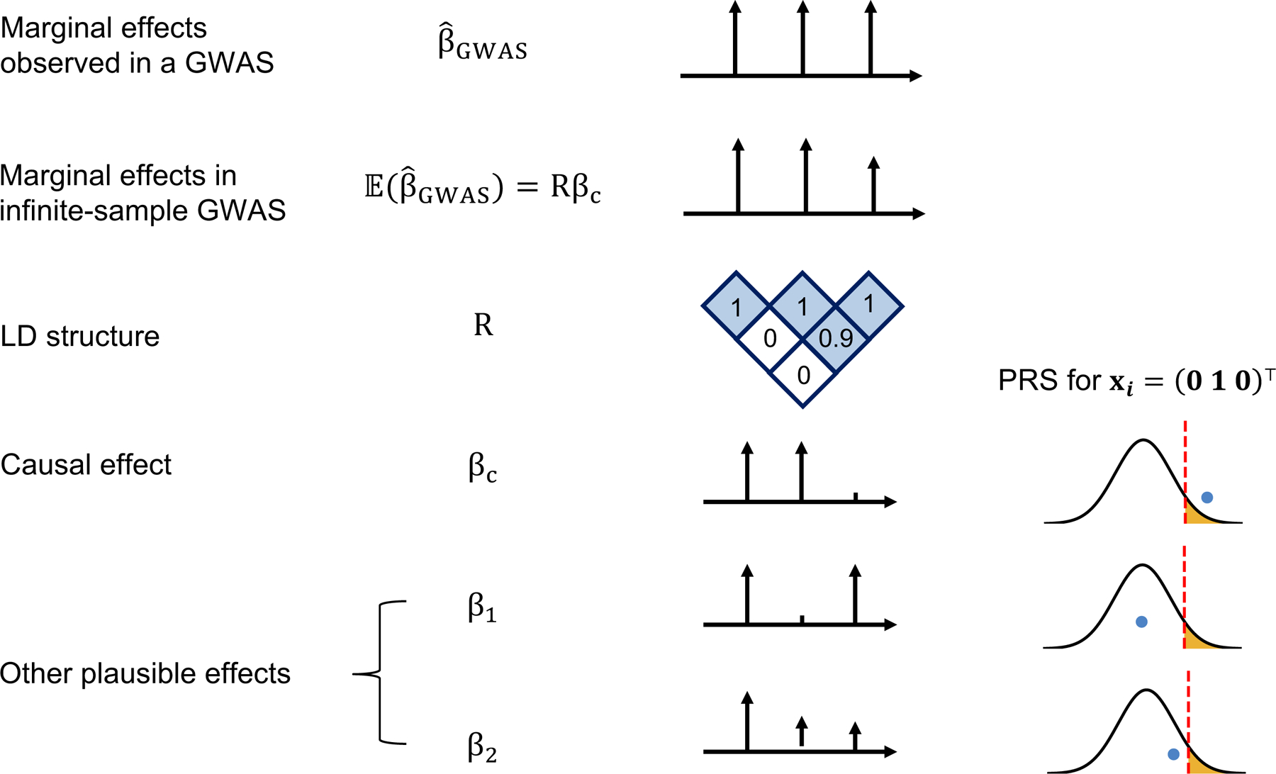
We simulated a GWAS of N individuals across 3 SNPs with LD structure R (SNP2 and SNP3 are in LD of 0.9 whereas SNP1 is uncorrelated to other SNPs) where SNP1 and SNP2 are causal with the same effect size β_c = (0.016, 0.016, 0) such that the variance explained by this region is var(x^⊤β_c) = 0.5/1000 corresponding to a trait with total heritability of 0.5 uniformly distributed across 1,000 causal regions. The marginal effects observed in a GWAS, ${\widehat{\beta }}_{\text{GWAS}}$, have an expectation of Rβ_c and variance-covariance $\left({\sigma }_{\text{e}}^2/\text{N}\right)R$, thus showcasing the statistical noise introduced by finite sample size of GWAS (N); for example, the probability of the marginal GWAS effect at tag SNP3 to exceed the marginal effect of true causal SNP2, although decreases with N, remains considerably high for realistic sample and effect sizes (12% at N=100,000 for a trait with h2=0.5 split across 1,000 causal regions, see Supplementary Figure 1). We consider one such observation for the effects observed in a GWAS: ${\widehat{\beta }}_{\text{GWAS}}=\left(0.016,0.016,0.016\right)$. Given such observation, in addition to the true causal effects (β_c), other causal configurations are probable β₁=(0.016, 0, 0.016) or β₂=(0.016, 0.008, 0.008). An individual with genotype x_i = (0 1 0)^⊤ will attain different PRS estimates under these different causal configurations. Most importantly, in the absence of other prior information, β₁ and β_c are equally probable given the data thus leading to different PRS estimates for individual x_i = (0 1 0)^⊤.

We explore inferential uncertainty in ${\widehat{\text{PRS}}}_i$ through two synergistic approaches. First, we provide a closed-form approximation for the expected $sd({\widehat{\text{PRS}}}_i)$ under simplifying assumptions. Second, we sample from the posterior distribution of the causal effects under the framework of LDPred2 to estimate $sd({\widehat{\text{PRS}}}_i)$ and compute credible intervals for GV_i at prespecified confidence levels (e.g., ρ = 95%) (Figure 2). As an example of the utility of such measures of uncertainty, we explore a probabilistic approach to PRS-based risk stratification that estimates the probability that GV_i is above a given threshold t (Figure 2) and demonstrate how this probability can be used in conjunction with situation-specific cost functions to optimize risk stratification decisions.

Figure 2. Framework for extracting uncertainty from Bayesian methods for probabilistic individual stratification.

(a) Procedure to obtain uncertainty from LDpred2. LDpred2 uses MCMC to sample from the posterior causal effect distribution given GWAS marginal effects, LD, and a prior on the causal effects. It outputs the posterior mean of the causal effects which is used to estimate the posterior mean genetic value (the PRS point estimate). Our framework samples from the posterior of the causal effects to approximate the posterior distribution of genetic value. The density plot represents the posterior distribution of GV for an individual. The shaded area represents a ρ-level credible interval. The dot represents the posterior mean. (b) Probabilistic risk stratification framework. Given a threshold t, instead of dividing individuals into above-threshold $\left({\widehat{\text{PRS}}}_i>t\right)$ and below-threshold $\left({\widehat{\text{PRS}}}_i\le t\right)$ groups dichotomously (left), probabilistic risk stratification assigns each individual a probability of being above-threshold (Pr(GV_i > t) (right).

Analytical derivation of individual PRS uncertainty

We focus on evaluating PRS uncertainty within a general Bayesian framework, where the posterior mean of the genetic effects conditional on a given GWAS, $\widehat{\beta }\equiv \mathbb{E}(\beta |D)$, is used to estimate the genetic value of a given individual, $x_i^{\top }\widehat{\beta }\equiv \mathbb{E}(x_i^{\top }\beta |D,x_i)$ (D = X,y) with access to individual data or $D=\left({\widehat{\beta }}_{\text{GWAS}},\widehat{R}\right)$ with access to marginal association statistics and LD, see Methods). We define PRS uncertainty for individual i as the posterior variance of their genetic value, $var(x_i^{\top }\beta |D,x_i)$. This quantity is an approximation to prediction error variance (PEV) of estimated breeding values (EBV) in livestock genetics^32,34, analogous to genetic value in human genetics (Methods).

Assuming that every SNP has a nonzero causal effect drawn i.i.d. from ${\beta }_j~N\left(0,\frac{h_g^2}{M}\right)$, one can derive a closed-form approximation to the expectation across individuals of the posterior variance of genetic value (Methods). Given a GWAS discovery dataset of N unrelated individuals drawn from a given population, the expected PRS uncertainty for a test individual i randomly drawn from the same population is

$${\mathbb{E}}_{x_i}\left[var\left(x_i^T\beta |D,h_g^2\right)\right]\approx {\left(\frac{1}{h_g^2}+\frac{N}{M}\right)}^{-1}$$ #(1)

Under an infinitesimal model, the analytical form is an approximately unbiased estimator of the expected posterior variance, even in the presence of LD (Figure 3a). Under non-infinitesimal models, the analytical form underestimates the expected posterior variance, albeit by a relatively small amount (Extended Data Figure 2). Notably, across 13 phenotypes in the UK Biobank, the analytical form provides relatively accurate estimates of the empirical average $\text{sd}({\widehat{\text{PRS}}}_{\text{i}})$ computed from LDpred2 posterior sampling (R² = 0.79 across traits, Figure 3b). Thus, the analytical form captures the interplay among SNP-heritability, sample size, and number of causal variants and provides a useful approximation to individual PRS uncertainty when posterior samples are unavailable.

Figure 3. Expected $sd({\widehat{\text{PRS}}}_i)$ estimated as a function of heritability, polygenicity and training GWAS sample size is highly correlated with average $sd({\widehat{\text{PRS}}}_i)$ across testing individuals.

(a) The analytical form provides approximately unbiased estimates of expected $\text{sd}({\widehat{\text{PRS}}}_{\text{i}})$ in simulations when p_causal = 1. The x-axis is the average $\text{sd}({\widehat{\text{PRS}}}_{\text{i}})$ in testing individuals. The y-axis is the expected $\text{sd}({\widehat{\text{PRS}}}_{\text{i}})$ computed from Equation (1). Each dot is an average of 10 simulation replicates for each ${\text{h}}_{\mathrm{g}}^2\in \left\{0.05,0.1,0.25,0.5,0.8\right\}$. The horizontal whiskers represent ± 1.96 standard deviations of average $\text{sd}({\widehat{\text{PRS}}}_{\text{i}})$ across 10 simulation replicates. The vertical whiskers represent ± 1.96 standard deviations of expected $\text{sd}({\widehat{\text{PRS}}}_{\text{i}})$ across 10 simulation replicates. (b) The analytical estimator of expected $\text{sd}({\widehat{\text{PRS}}}_{\text{i}})$ is highly correlated with estimates obtained via posterior sampling for real traits. The x-axis is the average $\text{sd}({\widehat{\text{PRS}}}_{\text{i}})$ in testing individuals. The y-axis is the expected $\text{sd}({\widehat{\text{PRS}}}_{\text{i}})$ computed from Equation (1), where M is replaced with the estimated number of causal variants and heritability is replaced with estimated SNP-heritability.

Factors impacting individual PRS uncertainty in simulations

Next, we quantified the degree to which different parameters contribute to uncertainty in individual PRS estimates in simulations starting from real genotypes of unrelated “white British” individuals in the UK Biobank (UKBB, N=291,273 individuals (N_train=250,000, N_validation=20,000, N_test=21,273) and M=459,792 SNPs, see Methods).

First, we assess the calibration of the ρ-level credible intervals for GV_i estimated by LDpred2. We compared the empirical coverage of the ρ-level credible intervals (proportion of individuals in a single simulation replicate whose ρ GV_i-CI overlaps their true GV_i) to the expected coverage (ρ) across a range of values of ρ. We find that, overall, the ρ GV_i-CI are well-calibrated, albeit slightly mis-calibrated in high-heritability, low-polygenicity simulations (Figure 4a and Extended Data Figure 3). For example, across 10 simulation replicates where $h_g^2=0.25$ and p_causal = 1%, the 95% GV_i-CIs have an average empirical coverage of 0.92 (s.e.m. 0.005) (Figure 4a). The ρ GV_i-CIs estimated by LDpred2 are also robust to training cohort sample size (Supplementary Figure 2). Since individuals with large PRS estimates might have larger number of effect alleles and therefore accumulate more inferential variance, we investigate whether individual PRS uncertainty varies with respect to their true genetic value and find no significant correlation between an individual’s $sd({\widehat{\text{PRS}}}_i)$ and their true genetic value (Figure 4b).

Figure 4. Genetic architecture (polygenicity (p_causal), SNP-heritability $\left(h_g^2\right)$, and GWAS sample sizes) impacts uncertainty in PRS estimates in simulations.

(a) Individual credible intervals are well-calibrated ($h_g^2=0.25$, p_causal = 1%). Empirical coverage is calculated as the proportion of individuals in a single simulation whose ρ-level credible intervals contain their true genetic risk. The dots and error bars represent mean ±1.96 s.e.m of the empirical coverage calculated from 10 simulations. (b) Correlation between uncertainty and true genetic value ($h_g^2=0.25$, p_causal = 1%). Each dot represents an individual. The x-axis is the true genetic value; the y-axis is standard deviation of the individual PRS estimate ($sd({\widehat{\text{PRS}}}_i)$). (c) Distribution of individual PRS uncertainty estimates with respect to polygenicity p_causal ∈ {0.0001, 0.01, 0.1, 1}, ($h_g^2=0.25$). Each violin plot represents $sd({\widehat{\text{PRS}}}_i)$ for 21,273 testing individuals across 10 simulations. (d) Distribution of individual PRS uncertainty estimates with respect to heritability ($h_g^2\in \left\{0.05,0.1,0.25,0.5,0.8\right\}$ p_causal = 0.01. Each violin plot represents scaled $sd({\widehat{\text{PRS}}}_i)$ for 21,273 testing individuals across 10 simulation replicates. Since larger heritability yields larger genetic values in our simulations, we plot $sd({\widehat{\text{PRS}}}_i)$ divided by the standard deviation of PRS point estimates in the testing group to enable comparison of uncertainty across different heritability values (Methods). (e) Distribution of individual uncertainty estimates with respect to training GWAS sample size. Each violin plot represents scaled $sd({\widehat{\text{PRS}}}_i)$ of individual PRS for 21,273 testing individuals across 10 simulation replicates.

We next assessed the impact of trait-specific genetic architecture parameters (heritability and polygenicity) on individual PRS uncertainty, defined as the posterior standard deviation of genetic value. First, we fixed heritability and varied polygenicity and found that $sd({\widehat{\text{PRS}}}_i)$ increases from 0.10 to 0.50 when the proportion of causal variants increases from 0.1% to 100% (Figure 4c, Extended Data Figure 4). Second, we varied the heritability while keeping polygenicity constant. Since different heritabilities lead to different variances explained by the PRS in the test sample, we scale the individual standard deviation ($sd({\widehat{\text{PRS}}}_i)$) by the standard deviation of PRS point estimates across all tested individuals; we refer to this quantity as “scaled SD” (Methods). We find that the scaled SD decreases with heritability and sample size (Figure 4d, Extended Data Figure 5). For example, when $h_g^2=0.05$ and p_causal = 0.1%, a 5-fold increase in training data sample size (50K to 250K) reduces scaled SD by 3-fold (from 1.50 to 0.56); when $h_g^2=0.05$ and p_causal = 1%, the same increase in training data sample size reduces the scaled SD by 4-fold (from 1.10 to 0.39). While the two simulation settings yield the same expected variance per causal variant under our simulation framework (i.e. $h_g^2/\left(M\times p_{\text{causal}}\right)$, see Methods), we observe lower uncertainty across all sample sizes for $h_g^2=0.5$ and p_causal = 1%, further emphasizing the impact of trait-specific genetic architecture on individual PRS uncertainty.

Next, we investigated the impact of different types of model misspecification on credible interval calibration and PRS uncertainty in simulations based on a set of 124,080 SNPs (the union of 36,987 UKBB array SNPs and 93,767 HapMap3 SNPs) on chromosome 2. First, we assessed the impact of imperfect tagging of causal variants by simulating phenotypes from the set of HapMap3 + UKBB SNPs (${\text{h}}_{\mathrm{g}}^2=0.02$, p_causal= 0.01, 0.001) and training the PRS on (i) 124,080 SNPs (HapMap3 + UKBB) and (ii) 36,987 SNPs (UKBB only). The “HapMap3 + UKBB” model contains all causal SNPs whereas the “UKBB only” model excludes ~70% of the causal SNPs, thus representing imperfect tagging of causal effects. As expected, the empirical coverage of the credible intervals is biased downward across a range of values of ρ when only the UKBB SNPs are used to train the model (Extended Data Figure 6). This downward bias is less pronounced when polygenicity is higher (e.g., p_causal = 0.01 vs 0.001) since the UKBB SNPs tag a larger proportion of heritability due to the increased causal SNP density. Second, to assess whether the coexistence of large and small causal effects impacts PRS uncertainty, we compared three simulation scenarios: (I) large effects only (p_causal= 0.001, $h_g^2=0.02$), (II) small effects only (p_causal = 0.01, $h_g^2=0.02$), and (III) a “mixture of normal” model (p_causal = 0.0055, $h_g^2=0.02$ in total) composed of large effects (p_causal = 0.0005, $h_g^2=0.01$) and small effects (p_causal = 0.005, $h_g^2=0.01$). We find that the presence of a large number of small effects increases the uncertainty in individual PRS estimates. For example, the average $\text{sd}({\widehat{\text{PRS}}}_{\text{i}})$ among the 21,273 test individuals is 0.050, 0.087, and 0.11 for simulations I, III and II, respectively (Extended Data Figure 7). In simulation III, both PRS uncertainty and accuracy (squared Pearson correlation between GV and PRS: $R_{\text{GV}}^2$ = 0.90, 0.51, 0.68 for I, II, III) are approximate averages of simulations I and II. Despite the LDpred2 model being mis-specified in the mixture of normal simulation, the genetic value credible intervals remain well-calibrated (Extended Data Figure 7). Third, we compared PRS obtained using external reference LD (a subsample of either 1,000 (1K) or 2,000 (2K) individuals held out from the UKBB training data) to those obtained using in-sample LD (all 250,000 individuals in the training data) and found similar degrees of PRS uncertainty and credible interval calibration (Extended Data Figure 8).

Individual PRS uncertainty in real data in the UK Biobank

We investigate individual PRS uncertainty across 13 traits in the UK Biobank: hair color, height, body mass index (BMI), bone mass density in the heel (BMD), high-density lipoprotein (HDL), low-density lipoprotein (LDL), cholesterol, igf1, creatinine, red blood cell count (RBC), white blood cell count (WBC), hypertension and self-reported cardiovascular disease (CVD). First we focus on PRS-based risk stratification. Since most traits analyzed here are not disease traits, we use “above-threshold” and “below-threshold” when referring to the results of risk stratification. We classify test individuals as above-threshold if their PRS point estimate (the posterior mean of their genetic value) exceeds a prespecified threshold t (i.e. ${\widehat{\text{PRS}}}_i>t$), where t is set to the 90^th PRS percentile obtained from the test-group individuals (Methods). (We note that this threshold was chosen arbitrarily to provide an example of how one can compute and interpret PRS uncertainty; in practice, choosing a threshold requires careful consideration of various trait-specific factors such as prevalence and the intended clinical application¹.) We then partition the above-threshold individuals into two categories: individuals whose ρGV_i-CI are fully above the threshold t (“certain above-threshold”) and individuals whose ρ GV_i-CI contain t (“uncertain above-threshold”). Similarly, we classify individuals with PRS estimates lie below a prespecified threshold into “certain below-threshold” and “uncertain below-threshold” categories (Figure 5a). At t = 90^th percentile and ρ = 95%, only 1.8% (s.d. 2.4%) of above-threshold individuals (averaged across traits) are deemed certain above-threshold individuals; the remaining above-threshold individuals have 95% GV_i − CI that overlap t (Figure 5b, Table 1). On the other hand, 33.7% (s.d. 15.3%) of below-threshold individuals have 95% GV_i − CI that do not overlap t (Figure 5b, Table 1). Consistent with simulations, we find that uncertainty is higher for traits that are more polygenic⁴⁵ (Table 1) with the average standard deviation of ${\widehat{\text{PRS}}}_i$ ranging between 0.2 to 0.41 across the studied traits (Table S1). We assessed the impact of quantile normalization of phenotypes and verify that for mildly skewed distributions, its impact on uncertainty is small (Supplementary Figures 3 and 4).

Figure 5. Uncertainty in real data and its influence on genetic risk stratification.

(a) Example of posterior PRS distributions for individuals with certain below-threshold (dark blue), uncertain below-threshold (light blue), uncertain above-threshold (light yellow), and certain above-threshold (dark yellow) classifications for HDL. Each density plot is a smoothed posterior PRS distribution of an individual randomly chosen from that category. The solid vertical lines are posterior means. The shaded areas are 95% credible intervals. The red dotted line is the classification threshold. (b) Distribution of classification categories across 11 traits (t=90%, ρ=95%). Each bar plot represents the frequency of testing individuals who fall into each of the four classification categories for one trait. The frequency is averaged across five random partitions of the whole dataset. (c) Correlation of PRS rankings of test individuals obtained from two MCMC samplings from the posterior of the causal effects. For each trait, we draw two samples from the posterior of the causal effects, rank all individuals in the test data twice based on their PRS from each sample, and compute the correlation between the two rankings across individuals. Each violin plot contains 5,000 points (1,000 pairs of MCMC samples and five random partitions).

Table 1. PRS-based individual stratification uncertainty across 11 complex traits in UK Biobank.

We quantified PRS-based stratification uncertainty in testing individuals for eleven complex traits at two stratification thresholds (t = 90^th and t = 99^th percentiles). The numbers of certain versus uncertain classifications are determined from the 95% credible intervals (ρ = 95%). For each trait, we report averages (and standard deviations) from five random partitions of the whole dataset.

Trait	PRS < t (“Below threshold”)		PRS > t (“Above threshold”)
	# Certain	# Certain/(#Certain + # Uncertain)	# Certain	# Certain/(#Certain + # Uncertain)
	t = 90 th
Hair color	11205.0 (287.0)	58.5 (1.5)%	131.4 (18.6)	6.2 (0.9)%
Height	5961.4 (197.6)	31.1 (1.0)%	18.4 (2.4)	0.9 (0.1)%
Body mass index (BMI)	935.8 (198.6)	4.9 (1.0)%	0.4 (0.5)	0.0 (0.0)%
High density lipoprotein (HDL)	5860.8 (681.9)	30.6 (3.6)%	16.2 (8.3)	0.8 (0.4)%
Low density lipoprotein (LDL)	8236.4 (494.3)	43.0 (2.6)%	29.6 (7.8)	1.4 (0.4)%
Cholesterol	7026.0 (660.1)	36.7 (3.4)%	20.2 (6.8)	0.9 (0.3)%
IGF1	3305.2 (371.8)	17.3 (1.9)%	4.0 (1.2)	0.2 (0.1)%
Creatinine	2052.4 (375.8)	10.7 (2.0)%	1.2 (1.3)	0.1 (0.1)%
Red blood cell count (RBC)	3745.8 (660.4)	19.6 (3.4)%	6.2 (3.6)	0.3 (0.2)%
White blood cell count (WBC)	1996.6 (120.5)	10.4 (0.6)%	0.6 (0.5)	0.0 (0.0)%
Bone mass density in heel (BMD)	1654.2 (152.5)	8.6 (0.8)%	2.0 (2.3)	0.1 (0.1)%
Hypertension	257.4 (78.1)	1.3 (0.4)%	0.0 (0.0)	0.0 (0.0)%
Cardiovascular (CVD)	125.4 (57.7)	0.7 (0.3)%	0.0 (0.0)	0.0 (0.0)%
Average (s.d.)	4027.9 (3398.3)	21.0 (17.8) %	17.7 (35.5)	0.8 (1.6) %
	t= 99th
Hair color	18398.6 (208.4)	87.4 (1.0)%	4.4 (1.5)	2.1 (0.7)%
Height	14442.6 (147.6)	68.6 (0.7)%	0.6 (0.9)	0.3 (0.4)%
Body mass index (BMI)	5254.4 (739.1)	24.9 (3.5)%	0.2 (0.4)	0.1 (0.2)%
High density lipoprotein (HDL)	14167.6 (691.4)	67.3 (3.3)%	0.2 (0.4)	0.1 (0.2)%
Low density lipoprotein (LDL)	15615.8 (448.1)	74.1 (2.1)%	0.6 (0.5)	0.3 (0.3)%
Cholesterol	14793.2 (668.3)	70.2 (3.2)%	0.2 (0.4)	0.1 (0.2)%
IGF1	11049.2 (597.9)	52.5 (2.8)%	0.2 (0.4)	0.1 (0.2)%
Creatinine	8337.2 (702.7)	39.6 (3.3)%	0.0 (0.0)	0.0 (0.0)%
Red blood cell count (RBC)	11532.8 (1056.9)	54.8 (5.0)%	0.0 (0.0)	0.0 (0.0)%
White blood cell count (WBC)	8496.6 (370.7)	40.3 (1.8)%	0.0 (0.0)	0.0 (0.0)%
Bone mass density in heel (BMD)	7816.0 (511.1)	37.1 (2.4)%	0.0 (0.0)	0.0 (0.0)%
Hypertension	2378.8 (390.7)	11.3 (1.9)%	0.0 (0.0)	0.0 (0.0)%
Cardiovascular (CVD)	1506.6 (512.3)	7.2 (2.4)%	0.0 (0.0)	0.0 (0.0)%
Average (s.d.)	10291.5 (5220.4)	48.9 (24.8) %	0.49 (1.2)	0.2 (0.6) %

For completeness, we investigated the impact of the threshold t, and credible level ρ, on PRS-based stratification uncertainty, defined as the proportion of above-threshold individuals classified as “certain above-threshold” for a given trait. As expected, the proportion of certain above-threshold classifications decreases as ρ increases (Figure 6a). For traits with higher average uncertainty (scaled SD) we observe lower rates of certain classifications across all values of ρ. For example, at t = 90^th and ρ = 95%, the proportion of above-threshold individuals classified with certainty is 0 % for BMI (average scaled SD = 1.54) and 6.2% for hair color (average scaled SD = 0.62) (Figure 6a). Height and HDL have similar average levels of uncertainty (average scaled SD of 0.95 for height and 0.96 for HDL) and similar proportions of above-threshold individuals classified with certainty (0.9% for height and 0.8% for HDL) (Figure 6a, Table 1). Using a more stringent threshold t amplifies the effect of uncertainty on PRS-based stratification (Figure 6b). For example, for BMI and hair color, the proportion of certain classifications among above-threshold individuals drops for all values of ρ when we increase the threshold from t=90^th percentile to t=99^th percentile (Figure 6b).

Figure 6. Stratification uncertainty at different threshold t and credible set level ρ.

(a) Proportion of above-threshold classifications that are “certain” for four representative traits. The x-axis shows ρ varying from 0 to 1 in increments of 0.05. The stratification threshold t is fixed at 90%. (b) Proportion of above-threshold classifications that are “certain” for two representative traits and two stratification thresholds (t = 90%, 99%). (c) Flexible cost optimization with probabilistic individual stratification under various cost functions. Each color corresponds to one cost function: (i) equal cost for each FP and FN diagnosis (C_FP = C_FN = 1, red); (ii) 3x higher cost for FP diagnoses (C_FP = 3, C_FN = 1, green); and (iii) 3x higher cost for FN diagnoses (C_FP = 1, C_FN = 3, blue). The probability threshold for classification is varied along the x-axis. Solid lines represent cost calculated using true genetic risk and dotted lines represent cost estimated from the probability of an individual being above-threshold. Diamond symbols represent the optimal classification threshold for each curve (the minima). Simulation parameters are fixed to $h_g^2=0.25$, p_causal = 1%.

We also quantified the impact of inferential variance in ${\widehat{\text{PRS}}}_i$ on PRS-based ranking of the test-group individuals. Using two random samples of genetic effects, we generated two independent rankings for all individuals in the test data and quantified the correlation in the rankings (Figure 5c, Methods). We observe large variability in the rankings across the test data, with the correlation of rankings ranging from 0.25 to 0.78 across the 13 traits. We also estimated 95% credible intervals for the rank of individuals at a given percentile (e.g., 90^th) (Table 2, Methods, Extended Data Figure 9) to find high variability in the ranking. For example, in the case of HDL an individual at 90^th (99^th) percentile based on PRS point estimate can be within 41^th to 99^th percentiles (72^th-99^th) with 95% probability when the inferential variance in PRS estimation is taken into consideration (Table 2).

Table 2. Average 95% posterior ranking credible intervals for individuals at two stratification thresholds for 11 traits.

We estimated the 95% posterior ranking credible intervals for individuals at the 90^th and 99^th percentiles of the testing population PRS estimates. Mean and standard deviation are calculated from the 95% posterior ranking intervals of individuals whose point estimates lie within 0.5% of the stratification threshold (213 individuals between the 89.5^th and 90.5^th percentiles for t = 90^th and between the 98.5^th and 99.5^th percentiles for t = 99^th).

Trait	t = 90th		t = 99th
	Lower bound	Upper bound	Lower bound	Upper bound
Hair color	57.9 (1.8)	97.9 (0.22)	88.0 (2.2)	99.8 (0.05)
Height	43.4 (2.1)	98.6 (0.18)	74.9 (3.4)	99.9 (0.04)
Body mass index (BMI)	22.9 (2.1)	99.0 (0.17)	45.8 (4.0)	99.8 (0.04)
High density lipoprotein (HDL)	41.3 (2.8)	98.7 (0.18)	72.3 (4.1)	99.9 (0.04)
Low density lipoprotein (LDL)	49.1 (2.4)	98.6 (0.19)	77.7 (3.5)	99.9 (0.04)
Cholesterol	45.1 (2.8)	98.6 (0.19)	74.9 (3.8)	99.9 (0.04)
IGF1	33.2 (2.4)	98.8 (0.17)	63.0 (4.1)	99.9 (0.04)
Creatinine	28.0 (2.4)	98.9 (0.17)	54.7 (4.3)	99.9 (0.04)
Red blood cell count (RBC)	34.5 (2.7)	98.8 (0.17)	64.4 (4.5)	99.9 (0.04)
White blood cell count (WBC)	28.2 (2.0)	98.9 (0.17)	56.0 (3.9)	99.9 (0.04)
Bone mass density in heel (BMD)	26.0 (2.2)	98.9 (0.18)	52.5 (4.1)	99.9 (0.04)
Hypertension	17.7 (1.8)	99.0 (0.17)	36.6 (3.4)	99.8 (0.05)
Cardiovascular (CVD)	15.5 (1.9)	99.0 (0.18)	32.3 (3.8)	99.8 (0.06)
Average (s.d.)	34.2 (12.9)	98.8 (.03)	61.0 (16.6)	99.9 (0)

Integrating uncertainty into PRS-based stratification

In contrast to current PRS-based stratification practices which compare an individual’s PRS point estimate, ${\widehat{\text{PRS}}}_{\text{i}}$, to a given threshold t, here we explore the use of the posterior probability that GV for individual i is above the threshold (i.e. Pr(GV_i > t)). We estimate Pr(GV_i > t) using Monte Carlo integration within the LDpred2 framework and show in simulations that the probability is well-calibrated for different causal effect size distributions despite slight miscalibration when polygenicity is high or causal variants are not present in the training SNP panel (Methods, Supplementary Figures 5 and 6).

As expected, for traits with higher PRS uncertainty, we observe a smaller proportion of testing individuals with deterministic classification (Pr(GV_i > t) = 0 or 1) (Extended Data Figure 10). We also find a tight correlation between ${\widehat{\text{PRS}}}_i$ and Pr(GV_i > t) across individuals in the test data (Extended Data Figure 10). This is due to the relatively high polygenicity of the traits in the analysis; a lower correlation is expected for traits with lower polygenicity (Supplementary Figure 7). However, Pr(GV_i > t) also contains information about individual-level false positive (FP) and false negative (FN) probabilities which, given a situation-specific cost function, can be used to calculate the expected cost of an above-threshold versus below-threshold classification (Methods). The cost functions for FP and FN should be carefully specified in the context of the clinical application; e.g., in the case of bone density scans, the cost functions will depend on the actual cost of a low bone density versus risks associated with exposure to low-dose x-rays. Consider three cost functions which relate the relative costs of false positive versus false negative diagnoses: (a) equal cost for each FP and FN diagnosis (C_FP = C_FN = 1); (b) 3x higher cost for FP diagnoses (C_FP = 3, C_FN = 1); and (c) 3x higher cost for FN diagnoses (C_FP = 1, C_FN = 3). For an individual with Pr(GV_i > t) = 0.6, the probability of a FP versus FN diagnosis is 0.4 versus 0.6, respectively. The expected costs of FP diagnoses (Pr(FP) × C_FP) under each scenario are (a) 0.4, (b) 1.2, and (c) 0.4; the expected costs of FN diagnoses (Pr(FN) × C_FN) are (a) 0.6, (b) 0.6, and (c) 1.8. Therefore, the classification for this individual that minimizes the expected cost under each scenario is (a) above-threshold, (b) below-threshold, and (c) above-threshold. More notably, since the probabilities are well-calibrated, we can estimate the expected cost for a population with the individual probability of being at above-threshold. As a demonstrating example, in simulation, we calculate the estimated cost curve on testing individuals (Methods), which is very close to the true cost curve despite slight inflation (Figure 6c). The estimated cost curves for the above-described cost functions achieve minimum cost at threshold = 0.5, 0.25 and 0.75 respectively, which is close to the optimum from true cost curves (0.5, 0.25, 0.7, Figure 6c).

Discussion

In this work, we demonstrate that uncertainty in PRS estimates at the individual level can have a large impact on subsequent analyses such as PRS-based risk stratification, which is complementary to methods that assess cohort-level metrics of PRS accuracy such as R². We propose a general procedure for obtaining estimates of individual-PRS uncertainty which can be applied to a wide range of existing PRS methods. Among 13 traits in the UK Biobank, we find that even with GWAS sample sizes on the order of hundreds of thousands of individuals, there is considerable uncertainty in individual PRS estimates that can impair the reliability of PRS-based stratification. We propose a probabilistic approach to stratification that can be used in conjunction with situation-specific cost functions to help inform PRS-based decision-making, noting that such an approach is not necessarily useful for all downstream applications of PRS. Since PRS must be combined with non-genetic risk factors (e.g., age, lab values) to evaluate an individual’s absolute risk for a given disease, the practical utility of PRS, including measures of uncertainty in PRS, is highly dependent on disease-specific factors such as heritability, age of onset, and the costs/risks that would be incurred by initiating treatment, among many others^1,3. We note that this work focuses on estimating genetic value rather than predicting the phenotype; uncertainty in predictions of phenotype will be larger than the results reported here by 1-$h_g^2$ due to the additional uncertainty in non-genetic factors⁴⁶, which can be further modeled and integrated^3,41,47–49. We conjecture that measures of individual-PRS uncertainty will be most useful for characterizing individuals whose combined risk scores (genetics + non-genetics factors) are at or close to the decision threshold for medical intervention; we leave an investigation of uncertainty in combined risk scores for future work.

We conclude with several caveats and future directions. First, we quantify individual PRS uncertainty by extending LDpred2²⁴, which is just one of many existing Bayesian methods that can be adapted for the same purpose^27,50,51. Extensions of other methods, including analogous procedures for P+T⁵² and regularization-based approaches^22,23 could also be investigated. Overall, our methods produce well-calibrated credible intervals in realistic simulation parameter ranges, albeit slight mis-calibration when polygenicity is low and heritability is high. We hypothesize that it is due to several approximations employed in LDpred2 for computational efficiency. We leave investigation of the impact of approximation on calibration and further improvement for future work.

Second, we propose an analytical form to estimate the expected PRS uncertainty as a function of GWAS sample size, number of causal SNPs and SNP-heritability. Although our analytical formula does provide a good approximation, systematic biases are observed, largely due to the ignorance of causal configuration uncertainty induced by LD. In practice, we recommend using samples from posterior distribution, whose properties are validated in our simulation studies.

Third, while we find broad evidence that both trait-specific genetic architecture parameters (e.g., heritability, polygenicity) and individual-specific genomic features (e.g., cumulative number of effect alleles) can impact individual PRS uncertainty, both sources of uncertainty merit further exploration. For example, we perform simulations under a model in which each causal variant explains an equal portion of total SNP-heritability but, in reality, genetic architecture can vary significantly among different traits. We do not find a correlation between an individual’s cumulative number of effect alleles and their individual PRS uncertainty. This is primarily due to the high polygenicity of the traits being tested. Consequently, we observe tight correlation between ${\widehat{\text{PRS}}}_i$ and Pr(GV_i > t) in most simulation scenarios except those with low polygenicity. Extending these analyses to traits with a wider range of genetic architectures will be of interest, for example, presence of both monogenic and polygenic disease risk factors^53,54. It’s also important to investigate the relative contribution of LD and small effect sizes to PRS uncertainty under various genetic architecture. We leave the method development of PRS uncertainty decomposition for future study.

Fourth, although we have shown that our approach is robust to certain types of model misspecification (e.g., mixture of normal effect sizes distributions, imperfect tagging of causal effects), we do not exclude the possibility of nonlinear interaction effects such as GxE, GxG and dominance effects^55–58. A comparison of the impact of genotype imputation on uncertainty also merits further exploration. We leave a full investigation of these questions for future work.

Lastly, in the present study, we did not investigate individual PRS uncertainty in transethnic or admixed population settings. Causal variants, causal effect sizes, allele frequencies, and LD patterns can vary significantly across populations^59,60. Moreover, PRS prediction accuracy (measured via cohort-level metrics) is well known to depend heavily on the ancestry of the individuals in the GWAS training data^61,62.We therefore leave a detailed exploration of individual PRS uncertainty with respect to ancestry as future work.

Methods

Individual PRS uncertainty.

Let y_i be a trait measured on the i-th individual, x_i an M × 1 vector of standardized genotypes and β an M × 1 vector of corresponding standardized effects for each genetic variant. Under a standard linear model, the phenotype model is $y_i=x_i^{\top }\beta +{ϵ}_i$, where ${ϵ}_i~N\left(0,{\sigma }_e^2\right)$. The goal of polygenic risk scores (PRS) methods is to predict genetic value for individual i $\left({\text{GV}}_i≔x_i^{\top }\beta \right)$ of the phenotype. In practice, the genetic effects β are unknown and need to be inferred from GWAS data as $\widehat{\beta }$. Therefore, the inferential variance in $\widehat{\beta }$ propagates to the estimated genetic value of individual i ${\widehat{\text{PRS}}}_i=x_i^{\top }\widehat{\beta }$. In this work we study the inferential variance in ${\widehat{\text{PRS}}}_i=x_i^{\top }\widehat{\beta }$ as a noisy estimate of ${\text{GV}}_i=x_i^{\top }\beta$

Estimating individual uncertainty in Bayesian PRS models.

Next, we show how Bayesian models for estimating ${\widehat{\text{PRS}}}_i$ can be extended to evaluate the variance of its estimate. We focus on LDpred2, a widely used method, although similar approach can be incorporated in most Bayesian approaches. LDpred2 assumes causal effects at SNP j are drawn from a mixture distribution with spike at 0 as follows:

$${\beta }_j~\{\begin{array}{cc}\mathcal{N}\left(0,\frac{h_g^2}{M{p}_{\text{causal}}}\right)& ,\text{ with probability}{p}_{\text{causal}}\\ 0& ,\text{ with probability }1-p_{\text{causal}}\end{array}$$

Here, M is the total number of SNPs in the model, $h_g^2$ is the heritability of the trait, and p_causal is the proportion of causal variants in the model (i.e., polygenicity). Let ${\widehat{\beta }}_{\text{GWAS}}$ and $\widehat{R}$ represent GWAS marginal effects and LD matrix computed from GWAS samples. By combining the prior probability $p(\beta |h_g^2,p_{\text{causal}})$ and the likelihood of observed data $p({\widehat{\beta }}_{\text{GWAS}}|\beta ,\widehat{R})$, we can compute a posterior distribution as $p\left(\beta |{\widehat{\beta }}_{\text{GWAS}},\widehat{R},h_g^2,p_{\text{causal}}\right)$. The posterior distribution is intractable and therefore LDpred2 uses Markov Chain Monte Carlo (MCMC) to obtain posterior samples from $p(\beta |{\widehat{\beta }}_{\text{GWAS}},\widehat{R},h_g^2,p_{\text{causal}})$. For simplicity, we use $\tilde{\beta }~p(\beta |{\widehat{\beta }}_{\text{GWAS}},\widehat{R},h_g^2,p_{\text{causal}})$ to refer to the samples from the posterior distribution, and use $p\left(\tilde{\beta }\right)$ to refer to $p(\beta |{\widehat{\beta }}_{\text{GWAS}},\widehat{R},h_g^2,p_{\text{causal}})$ whenever context is clear. The posterior samples of the causal effects are summarized using the expectation $\mathbb{E}\left[\tilde{\beta }\right]=\int \tilde{\beta }p\left(\tilde{\beta }\right)d\tilde{\beta }$, leading to ${\widehat{\text{PRS}}}_i=x_i^{\top }\mathbb{E}\left[\tilde{\beta }\right]$.

Unlike existing methods that summarize the posterior samples of causal effects into the expectation and then estimate ${\widehat{\text{PRS}}}_i$, we sample from the posterior of PRS_i to construct a ρ level credible interval of genetic value (ρ GV_i-CI) for each individual. Bernstein-von Mises theorem provides the basis that under certain conditions, such constructed Bayesian credible interval will asymptotically be of coverage probability ρ⁶³. This property of the Bayesian credible interval provides intuitive explanation of the uncertainty. Concretely, we obtain B MCMC samples from the posterior distribution of causal effects $p\left(\tilde{\beta }\right):{\tilde{\beta }}^{\left(1\right)},{\tilde{\beta }}^{\left(2\right)},\dots ,{\tilde{\beta }}^{\left(B\right)}$. Then we compute a PRS estimate for individual i from each sample of $p\left(\tilde{\beta }\right):x_i^{\top }{\tilde{\beta }}^{\left(1\right)},x_i^{\top }{\tilde{\beta }}^{\left(2\right)},\dots ,x_i^{\top }{\tilde{\beta }}^{\left(B\right)}$ to approximate the posterior distribution of PRS_i ($p\left(x_i^{\top }\tilde{\beta }\right)$). From the B samples of posterior, we obtain empirical $\frac{1-\rho }{2}$ and $\frac{1-\rho }{2}$ quantiles as lower and upper bound estimates of ρ GV_i-CI (Figure 2b). As B goes to infinity, such Monte Carlo estimates converge to the $\left[Q_{\left(1-\rho \right)/2}\left(x_i^{\top }\tilde{\beta }\right),Q_{\left(1+\rho \right)/2}\left(x_i^{\top }\tilde{\beta }\right)\right]$, where $Q_{\alpha }\left(x_i^{\top }\tilde{\beta }\right)$ represents the α-quantile (here, α = (1−ρ)/2, (1+ρ)/2) for distribution of $p\left(x_i^{\top }\tilde{\beta }\right)$. Similarly, we summarize the posterior samples using the second moment to estimate $sd({\widehat{\text{PRS}}}_i)=sd\left(x_i^{\top }\tilde{\beta }\right)$. In practice, we used B = 500 as that leads to stable results. We investigated the autocorrelation statistics and found no evidence of autocorrelation at various lags in our experiment. (Supplementary Figure 8). We recommend checking autocorrelation in practice. The MCMC samplings should be thinned when there is strong evidence of autocorrelation, which otherwise will lead to underestimation of variance.

Although in this work we focus on LDpred2, the above described procedure is generalizable to a wide range of Bayesian methods (e.g., SBayesR²⁷, PRS-CS⁵⁰ and AnnoPred⁵¹). Methods that are not based on Bayesian principle could potentially use Bootstrap to obtain individual uncertainty intervals⁶⁴.

PRS uncertainty analytical form under infinitesimal model.

To facilitate understanding of PRS uncertainty, we derive an analytical estimator of PRS uncertainty under simplified assumptions: (1) all M SNPs are independent and causal; and (2) effect sizes are i.i.d. and drawn from an infinitesimal model, ${\beta }_j~N\left(0,h_g^2/M\right)$ for j=1,…, M, where $h_g^2$ is the total heritability and M is the number of causal variants. Without loss of generality, we assume that genotypes are standardized to have mean zero and unit variance in the population, i.e. $\mathbb{E}\left(x_{ij}\right)=0$ and var(x_ij) = 1, where x_ij is the genotype at SNP j for individual i. Under this assumption, following Appendix A in ref.²⁶, the least squares estimate of the GWAS marginal effect ${\widehat{\beta }}_{\text{GWAS},j}$ is approximately distributed as

$${\widehat{\beta }}_{\text{GWAS},j}|{\beta }_j~N\left({\beta }_j,\frac{1}{N}\left(1-\frac{h_g^2}{M}\right)\right).$$

Since the per-SNP heritability in this model, $\frac{h_g^2}{M}$, is small, the variance $\frac{1}{N}\left(1-\frac{h_g^2}{M}\right)$ can be approximated as 1/N. The posterior distribution of ${\beta }_j|{\widehat{\beta }}_{\text{GWAS},j}$ then becomes

$${\beta }_j|{\widehat{\beta }}_{\text{GWAS},j}~\text{N}\left({\left(1+\frac{M}{h_g^{2}N}\right)}^{-1}{\widehat{\beta }}_{\text{GWAS},j},\frac{1}{N}{\left(1+\frac{M}{h_g^{2}N}\right)}^{-1}\right).$$

Therefore, the posterior variance of genetic value for an individual with the genotype x_i can be approximated as

$$var\left(x_i^{\top }\beta |x_i,X,y,h_g^2\right)\approx \sum _{j=1}^M{x}_{ij}^{2}var\left({\beta }_j|{\widehat{\beta }}_{\text{GWAS},j}\right)=\frac{{\sum }_{j=1}^M{x}_{ij}^2}{N}{\left(1+\frac{M}{h_g^{2}N}\right)}^{-1},$$

where the approximation is based on the fact that β_j and β_k are approximately independent in the posterior distribution.

Recalling that genotype is standardized so that $\mathbb{E}(x_{ij}^2)=1$, the expected posterior variance of genetic value in the population can be approximated by:

$${\mathbb{E}}_{x_i}\left(var\left(x_i^{\top }\beta |x_i,X,y,h_g^2\right)\right)\approx \frac{M\mathbb{E}\left(x_{ij}^2\right)}{N}{\left(1+\frac{M}{h_g^{2}N}\right)}^{-1}={\left(\frac{1}{h_g^2}+\frac{N}{M}\right)}^{-1}$$

Connection between PEV and posterior variance.

Prediction error variance (PEV), a widely used concept in the animal breeding literature, is defined as $va{r}_{\beta ,y}\left[x_i^{\top }\widehat{\beta }-x_i^{\top }\beta \right]$, where x_i is the genotype of individual i and $\widehat{\beta }={\mathbb{E}}_{\beta |y}\left[\beta \right]$ is the posterior mean of the causal effects. This variance is with respect to the randomness of both the prior β and phenotype y, conditional on a fixed genotype matrix X. Furthermore, assumptions can be made on X, to incorporate the randomness in X. PRS uncertainty with X fixed, which we derive here, will be a lower bound for PRS uncertainty with random X.

It follows from the law of total variance that $va{r}_{\beta ,y}\left[\beta \right]={\mathbb{E}}_y\left[va{r}_{\beta |y}\left[\beta \right]\right]+va{r}_y\left[{\mathbb{E}}_{\beta |y}\left[\beta \right]\right]$. Using the fact that $va{r}_{\beta ,y}\left[\widehat{\beta }-\beta \right]=va{r}_{\beta ,y}\left[\beta \right]-va{r}_{\beta ,y}\left[\widehat{\beta }\right]$ (Section 5.6.4 from ref.³¹), we have

$$\begin{gathered} va{r}_{\beta ,y}\left[\widehat{\beta }-\beta \right]=va{r}_{\beta ,y}\left[\beta \right]-va{r}_{\beta ,y}\left[\widehat{\beta }\right] \\ ={\mathbb{E}}_y\left[va{r}_{\beta |y}\left[\beta \right]\right]+va{r}_y\left[{\mathbb{E}}_{\beta |y}\left[\beta \right]\right]-va{r}_{\beta ,y}\left[\widehat{\beta }\right] \\ ={\mathbb{E}}_y\left[va{r}_{\beta |y}\left[\beta \right]\right] \end{gathered}$$

Finally, by multiplying a fixed genotype vector x_i to both sides, we have

$$va{r}_{\beta ,y}\left[x_i^{\top }\widehat{\beta }-x_i^{\top }\beta \right]={\mathbb{E}}_y\left[va{r}_{\beta |y}\left[x_i^{\top }\beta \right]\right]$$

Therefore, the posterior variance is an unbiased estimator of prediction error variance. We also note that under infinitesimal model setting, the posterior variance of genetic value has the same matrix form as the inversion of coefficient matrix of mixed model equation for BLUP^30,33.

Simulations.

We design simulation experiments in various settings and different sample sizes to understand the properties of uncertainty in PRS estimates. We used simulation starting from genotypes in UK Biobank⁶⁵. We excluded SNPs with MAF < 0.01 and genotype missingness > 0.01, and those SNPs that fail the Hardy-Weinberg test at significance threshold 10⁻⁷, which leaves us 459,792 SNPs. We preserve “white British individual”, with self-reported British white ancestry and filter pairs of individuals with kinship coefficient < 1/2^(9/2))⁶⁵. We further filtered individuals who are outliers for genotype heterozygosity and/or missingness, and obtained 291,273 individuals for all analyses.

Given the genotype matrix X, heritability $h_g^2$, proportion of causal variants p_causal, standardized effects and phenotypes are generated as follows

$${\beta }_j~\{\begin{array}{cc}N\left(0,\frac{h_g^2}{M{p}_{\text{causal}}}\right)& {\text{c}}_{\mathrm{j}}=1,\text{ with probability }{p}_{\text{causal}}\\ 0& {\text{c}}_{\mathrm{j}}=0,\text{ with probability }1-p_{\text{causal}}\end{array}$$

$${\left(y_1,\dots ,y_N\right)}^{\top }~N\left(X\beta ,\left(1-h_g^2\right)I_N\right)$$

Finally, given the phenotypes y = (y₁,…y_N)^⊤ and genotypes X, we simulate the GWAS marginal association statistics with ${\widehat{\beta }}_{\text{GWAS}}=\frac{1}{N}{X}^{\top }y$. We simulate the data using a wide range of parameters, $h_g^2\in \left\{0.05,0.1,0.25,0.5,0.8\right\}$, p_causal ∈ {0.001,0.01,0.1,1}, a total of 20 simulation settings, with each repeated 10 times. The total population of individuals is randomly assigned to 250,000 individuals as the training population, 20,000 individuals as the validating population, and the rest of 21,273 individuals as the testing population, as the usual practice for the PRS model building process. When investigating how sample sizes in the training cohort change PRS uncertainty, we vary the sample sizes in the training population in 20,000, 50,000, 100,000, 150,000, and 250,000, while holding the validation population and testing population as intact, to enable a fair comparison between sample sizes.

Real data analysis.

We performed real data analysis with 13 real traits from UK Biobank, including hair color, height, body mass index (BMI), bone mass density in the heel (BMD), high density lipoprotein (HDL), low density lipoprotein (LDL), cholesterol, igf1, creatinine, red blood cell count (RBC) and white blood cell count (WBC), hypertension and cardiovascular disease. The genotype was processed in the same way as the simulation study, where we have 459,792 SNPs and 291,273 individuals. We randomly partitioned the total of 291,273 individuals into 250,000 training, 20,000 validation and 21,273 testing groups. Training samples were used to estimate PRS weights; validation samples were used to estimate hyperparameters (e.g., heritability and polygenicity) for LDpred2; and testing samples were used to evaluate accuracy and uncertainty. The random partition was repeated five times to average of the randomness of results due to sample partition. For each round of random partition of the individuals, we calculated marginal association statistics between genotype and quantile-normalized phenotype in training group with PLINK, using age, sex, and the first 20 genetic principal components as the covariates. Then we applied LDpred2 to obtain the individual posterior distribution of the genetic value, as described above. We regressed out covariates from the phenotypes to obtain adjusted phenotypes, where the regressing coefficients are first estimated from the training population, and applied to phenotype from training, validation and testing population respectively. We evaluate accuracy of PRS estimates in validation and testing groups by Pearson correlation between PRS estimates and adjusted phenotypes.

PRS analysis using LDpred2.

We run LDpred2 for both simulation and real data analysis with the following settings. We calculate the in-sample LD with functions provided by the LDpred2 package, using the window size parameter of 3cM. We estimate the heritability $h_{{\text{chr}}_i}^2,i=1,\dots ,22$ for each chromosome with built-in constrained LD score regression⁶⁶ function. We run LDpred2-grid per chromosome with a grid of 17 polygenicity parameters p_causal from 10⁻⁴ to 1 equally spaced in log space, three heritability parameters $\left\{0.7h_{{\text{chr}}_i}^2,1.0h_{{\text{chr}}_i}^2,1.4h_{{\text{chr}}_i}^2\right\}$, and with the sparsity option both enabled and disabled, as recommended by LDpred2. We choose the model with the highest R² between the predicted posterior mean and the (adjusted) phenotype on validation set as best model to apply to testing data. We extract 500 posterior samples of causal effects ${\tilde{\beta }}^{\left(1\right)},{\tilde{\beta }}^{\left(2\right)},\dots ,{\tilde{\beta }}^{\left(500\right)}$ after 100 burn-in iterations from MCMC sampler of the model to approximate posterior distribution of causal effects. For each individual with genotype x_i, we calculate $x_i^{\top }{\tilde{\beta }}^{\left(1\right)},x_i^{\top }{\tilde{\beta }}^{\left(2\right)},\dots ,x_i^{\top }{\tilde{\beta }}^{\left(500\right)}$ to approximate GV posterior distribution for individual i. We then calculate summary statistics of GV posterior distribution, including the posterior mean $({\widehat{\text{PRS}}}_i)$, ρ level credible interval (ρ GV_i-CI) and probability of above threshold t (Pr(GV_i > t)).

Calculating and evaluating the coverage.

We evaluate the coverage properties of ρ GV_i-CI in simulation: we check whether $\mathbb{P}\left(x_i^{\top }\beta \in \left[Q_{\left(1-\rho \right)/2}\left(x_i^{\top }\tilde{\beta }\right),Q_{\left(1+\rho \right)/2}\left(x_i^{\top }\tilde{\beta }\right)\right]\right)=\rho$. To evaluate this property, for each simulated dataset, we calculate the frequency of the true genetic risk lies in the predicted interval, i.e., the frequency of $x_i^{\top }\beta \in \left[Q_{\left(1-\rho \right)/2}\left(x_i^{\top }\tilde{\beta }\right),Q_{\left(1+\rho \right)/2}\left(x_i^{\top }\tilde{\beta }\right)\right]$ for every individual in the testing population, for ρ ∈ {0.1, 0.2, …, 1.0}. This property provides us an intuitive understanding of the predicted interval: for an individual with a predicted interval $\left[Q_{\left(1-\rho \right)/2}\left(x_i^{\top }\tilde{\beta }\right),Q_{\left(1+\rho \right)/2}\left(x_i^{\top }\tilde{\beta }\right)\right]$, its true genetic risk is expected to be in this interval with a probability ρ.

Scaled standard deviation in individual PRS estimates.

To compare the relative order of standard deviation across different genetic architecture, especially across genetic architecture with different heritability, we define the quantity, scaled standard deviation in individual PRS estimates (scaled $sd({\widehat{\text{PRS}}}_i)$) to enable fair comparison. The quantity is defined for every individual i, as ${\text{sd}}_{\tilde{\beta }}\left[x_i^{\top }\tilde{\beta }\right]/{\text{sd}}_{x_i}\left[x_i^{\top }\widehat{\beta }\right]$, where the numerator term ${\text{sd}}_{\tilde{\beta }}\left[x_i^{\top }\tilde{\beta }\right]$ refers to standard deviation due to the posterior sampling of $\tilde{\beta }$ of i-th individual. Recalling that $x_i^{\top }\widehat{\beta }=\mathbb{E}\left[x_i^{\top }\tilde{\beta }\right]$, the denominator term ${\text{sd}}_{x_i}\left[x_i^{\top }\widehat{\beta }\right]$ refers to the variation of the point estimate across individuals in the population.

Posterior individual ranking interval.

The relative rank of individual PRS $x_i^{\top }{\tilde{\beta }}^{\left(\text{b}\right)}$ in the population $x_j^{\top }{\tilde{\beta }}^{\left(\text{b}\right)},j=1,\dots ,N$ varies across different MCMC samplings of posterior causal effects. To evaluate the uncertainty of ranking for individual i, we compute $r_i^{\left(b\right)}$ as the quantile of $x_i^{\top }{\tilde{\beta }}^{\left(\text{b}\right)}$ in the population $x_j^{\top }{\tilde{\beta }}^{\left(\text{b}\right)},j=1,\dots ,N$ for each of the b = 1, …, B posterior samples to approximate posterior distribution of the relative rank. We can obtain ρ-level credible intervals of ranking as [Q_(1−ρ)/2(r_i), Q_(1+ρ)/2(r_i)] for each individual i. To assess the uncertainty of ranking for individuals at 90 (99) percentile threshold based on PRS estimates, we select individuals within 1 percentile of thresholds (89.5–90.5%, 98.5–99.5%) and compute mean and standard deviation for lower and upper bound of ρ=95% posterior ranking interval, across the selected individuals.

PRS rank correlation between MCMC samplings.

With the B posterior causal effects samples ${\tilde{\beta }}^{\left(1\right)},{\tilde{\beta }}^{\left(2\right)},\dots ,{\tilde{\beta }}^{\left(B\right)}$ after burn-in, and N individuals in the testing population x₁, x₂, …, x_N, we compute PRS for each individual, $x_1^{\top }{\tilde{\beta }}^{\left(b\right)},\dots ,x_N^{\top }{\tilde{\beta }}^{\left(b\right)}$ and its relative rank in the population $r_1^{\left(b\right)},\dots ,r_N^{\left(b\right)}$ for each posterior sample ${\tilde{\beta }}^{\left(b\right)}$. Then for each pair of different b₁-th,b₂-th posterior samples, ${\tilde{\beta }}^{\left(b_1\right)},{\tilde{\beta }}^{\left(b_2\right)}$, we calculate the spearman correlation between $r_1^{\left(b_1\right)},\dots ,r_N^{\left(b_1\right)}$ and $r_1^{\left(b_2\right)},\dots ,r_N^{\left(b_2\right)}$, representing the variability of the ranks across MCMC samplings. We compute the rank correlation for 1000 pairs of different MCMC samplings, and get the distribution of the rank correlation.

Probabilistic risk stratification.

We define the notion of probabilistic framework for risk stratification based on posterior distribution of GV_i. Given a pre-specified threshold t, for every individual, we can calculate the posterior probability of the genetic risk larger than the given threshold t, (Pr(GV_i > t), with Monte Carlo integration as

$$\text{Pr}\left({\text{GV}}_i>t\right)=\frac{1}{B}\sum _{b=1}^B\mathbb{I}(x_i^{\top }{\tilde{\beta }}^{\left(b\right)}>\text{t})$$

We use the previous simulation settings to show that this probability is well calibrated. For each simulation, we divide the individuals based on their posterior probability of being at above-threshold into 10 bins with {0, 0.1, …, 1.0} as breaks. For each bin, we calculate the proportion of individuals with true genetic risk higher than the threshold as the empirical probability and the average posterior probability as theoretical probability. The empirical probability is expected to be the same as theoretical probability.

Integrating uncertainty into PRS-based stratification.

The individualized posterior distribution of genetic value provides extra information for patient stratification. We consider a scenario that there is a cost associated for decision that (1) classify an individual with low genetic risk into a high genetic risk category, C_FP, where FP represents false positive. (2) classify an individual with high genetic risk into a low genetic risk category, C_FN, where FN represents false negative. For an individual with posterior probability (Pr(GV_i > t), we want to decide an action, whether to classify this individual to be at high genetic risk, and perform further screening. If we classify this individual as above-threshold, we will have probability 1−(Pr(GV_i > t), that this individual is in fact below-threshold, inducing an expected cost C_FP(1−(Pr(GV_i > t)). Conversely, if we classify this individual as below-threshold, we will have probability (Pr(GV_i > t) that this individual will be in the high genetic risk, inducing an expected cost C_FN(Pr(GV_i > t). To minimize the expected cost, we would decide according to which action leads to the least cost. The critical value in this scenario is $\frac{C_{\text{FN}}}{C_{\text{FP}}+C_{\text{FN}}}$: if $\text{Pr}\left({\text{GV}}_i>t\right)>\frac{C_{\text{FN}}}{C_{\text{FP}}+C_{\text{FN}}}$, we would choose to classify this individual as above-threshold, otherwise below-threshold. For Figure 6c, given the cost parameters C_FP, C_FN, and a threshold t, for every decision threshold, we calculate the estimated cost by summing up C_FP(1-(Pr(GV_i > t)) for those individuals classified as high genetic risk category, and C_FN(Pr(GV_i > t) for those individuals classified as low genetic risk category in the testing data. Correspondingly, for every decision threshold, we also calculate the true cost based on the ground truth of genetic values in the simulation.

Software implementation.

Our method is implemented in the LDpred2 package (see URLs). In the function `snp_ldpred2_grid`, setting the option `return_sampling_betas = TRUÈ will output B posterior samples of the causal genetic effects. Posterior samples of an individual’s GV are obtained by multiplying the individual’s genotype by the M × B weight matrix. One can subsequently obtain the posterior mean, posterior variance, and other quantities of interest from the posterior of the GV. We note that the time required to estimate the causal effects remains the same; the only additional computational costs come from storing the M × B weight matrix and from multiplying the genotype vector by an M × B matrix rather than an M × 1 vector. The memory required to store 500 samples of causal effects for 459,792 SNPs is approximately 2 GB. Given the B posterior samples of causal effects, the runtime for computing the posterior distribution of genetic value for 10,000 testing individuals is less than five minutes.

Extended Data

Extended Data Fig. 1. GWAS sample size and causal effect size impact the relative ordering of marginal GWAS effects at tag versus true causal SNPs.

We simulated a GWAS of N individuals (X_N×3) for 3 SNPs with LD structure R (SNP2 and SNP3 are in LD of 0.9 whereas SNP1 is uncorrelated to other SNPs) where SNP1 and SNP2 are causal with the same effect size β_c = (β, β, 0) such that the variance explained by this region is var (Xβ_c) = 0.5/m_causal corresponding to a trait with total heritability of 0.5 equally distributed across m_causal regions in the genome. For each parameter setting we quantified the proportion of times the marginal GWAS effect at SNP3 (tag SNP) is larger than the observed marginal effect at SNP2 (true causal) across 1,000 randomly drawn GWASs. To explore the impact of different causal effect sizes, we varied m_causal from 1,000 to 10,000 causal regions in the genome.

Extended Data Fig. 2. Analytical estimator of $\text{sd}({\widehat{\text{PRS}}}_{\text{i}})$ provides an approximately unbiased estimates of average sd(PRSi) of testing individuals.

The x-axis is the average $\text{sd}({\widehat{\text{PRS}}}_{\text{i}})$ in testing individuals within each simulation replicate. The y-axis is the expected $\text{sd}({\widehat{\text{PRS}}}_{\text{i}})$ computed with Equation (1), replacing M and $h_g^2$ with estimates of the number of causal variants and SNP-heritability, respectively, from LDpred2. Each dot is an average of 10 simulation replicates for each p_causal ∈ {0.001, 0.01, 0.1, 1}. The horizontal whiskers represent ± 1.96 standard deviations of average $\text{sd}({\widehat{\text{PRS}}}_{\text{i}})$. The vertical whiskers represent ± 1.96 standard deviations of expected $\text{sd}({\widehat{\text{PRS}}}_{\text{i}})$. Note that when p_causal = 1, the independent LD assumption is violated but the analytical form still provides approximately unbiased estimates. When p_causal ≠ 1, the infinitesimal assumption is violated, leading to downward bias in the analytical estimator. In these scenarios, since we simply replace M with M × p_causal, the uncertainty identifying the causal variants is ignored by Equation (1).

Extended Data Fig. 3. Calibration of ρ-level genetic value credible interval with respect to proportion of causal effects and SNP-heritability in testing individuals.

Each row of panels corresponds to one heritability parameter $h_g^2\in \left\{0.05,0.1,0.25,0.5,0.8\right\}$ and each column of panels corresponds to one polygenicity parameter p_causal ∈ {0.001, 0.01, 0.1 1}. The x-axis is the expected coverage of ρ-GV CI (ρ). The y-axis is the empirical coverage calculated as the proportion of ρ-GV CIs that contain the true genetic value for one simulation repeat. The dots and error bars are mean ± 1.96 s.e.m of the empirical coverage calculated from 10 simulation repeats.

Extended Data Fig. 4. Distribution of individual PRS absolute standard deviation with respect to polygenicity under different heritability.

Each panel represents simulation with one $h_g^2$ from {0.05, 0.1, 0.25, 0.5, 0.8}. The x-axis is four polygenicity parameters (p_causal ∈ {0.001, 0.01, 0.1, 1}). The y-axis is standard deviation in PRS estimation of an individual. Each violin plot represents 21,273 testing individuals across 10 simulations (212,730 values).

Extended Data Fig. 5. Distribution of individual PRS absolute standard deviation with respect to heritability under different polygenicity.

Each panel represents simulation with one polygenicity from {0.001, 0.01, 0.1, 1}. The x-axis is five heritability parameters ($h_g^2\in \left\{0.05,0.1,0.25,0.5,0.8\right\}$). The y-axis is scaled standard deviation in PRS estimation of an individual. Each violin plot represents 21,273 testing individuals across 10 simulations (212,730 values).

Extended Data Fig. 6. Posterior distribution of genetic value is mis-calibrated when causal variants are partially absent in the SNP panel used for PRS training.

For all panels, we simulated 124,080 SNPs (a union of 36,987 UK Biobank (UKBB) array SNPs and 93,767 HapMap3 SNPs) on chromosome 2. We trained the PRS model on either the HapMap3 + UKBB SNPs (all causal variants are observed in the training data) or UKBB SNP panel (~70% of causal variants are excluded). (a) Calibration of ρ-level genetic value credible interval. The x-axis is the expected coverage of ρ-GV CI (i.e. ρ). The y-axis is the empirical coverage calculated as the proportion of GV CIs that contain the true genetic value in one simulation replicate. (b) Calibration of ρ-level rank credible interval. The x-axis is the expected coverage of the rank CI (ρ). The y-axis is the empirical coverage calculated as the proportion of ρ-rank CIs that contain the true rank of individual among testing individuals in one simulation replicate. (c) Calibration of probability of GV above threshold t. The x-axis is the expected probability set as middle of each bin. The y-axis is the empirical probability calculated as the proportion of individuals having GV within the lower and upper bound of the bin of one simulation replicate. Different colors represent different prespecified thresholds. (d) Distribution of individual PRS scaled standard deviation. For (a-c), the dots and error bars are mean ± 1.96 s.e.m empirical coverage/probability calculated from 10 simulation replicates. For (d), the boxplot center line is the median; the lower and upper hinges correspond to the first and third quartiles, and boxplot whiskers extend to the minimum and maximum estimates located within 1.5 × interquartile range (IQR) from the first and third quartiles, respectively.

Extended Data Fig. 7. Posterior distribution of genetic value is well-calibrated for mixture of normal effect size distribution.

Each column summarizes results for each of the three genetic architectures. Small effects are simulated under pcausal = 0.01, h2g = 0.02; large effects are simulated under pcausal = 0.001, h2g = 0.02; Mixture refers to a half and half mixture of the two simulations (small effects: pcausal = 0.0005, h2g = 0.01; large effects: pcausal = 0.005, h2g = 0.01). (a) Calibration of ρ-level genetic value credible intervals. (b) Calibration of ρ-level rank credible intervals. (c) Calibration of probability of GV above threshold t. (d) Distribution of individual PRS standard deviations. See Extended Data Figure 6 for a detailed figure description.

Extended Data Fig. 8. Posterior distribution of genetic value is well-calibrated with external LD.

Each column summarizes the calibration and uncertainty of PRS trained with LD computed from four different cohorts: I. 250K UKB training individuals; II. 2K held-out UKBB individuals; III. 1K held-out UKBB individuals. (a) Calibration of ρ-level genetic value credible intervals. (b) Calibration of ρ-level rank credible intervals. (c) Calibration of probability of GV above threshold t. (d) Distribution of individual PRS scaled standard deviation. See Extended Data Figure 6 for a detailed figure description (h²_g = 0.02, p_causal= 0.01).

Extended Data Fig. 9. Calibration of ρ-level rank credible interval with respect to proportion of causal effects and SNP-heritability in testing individuals.

The x-axis is the expected coverage of ρ-Rank CI. The y-axis is the empirical coverage calculated as the proportion of ρ-Rank CIs that contain the true rank of individual among testing individuals for one simulation. The dots and bars are mean ± 1.96 s.e.m of empirical coverage calculated from 10 simulation repeats.

Extended Data Fig. 10. Individual ranking is consistent when ranking by PRS estimates versus probability of genetic value above threshold.

The x-axis is the PRS estimates of testing individuals and the y-axis is the probability that GV is above threshold t, where t is (arbitrarily) set to the 90th percentile in the testing individuals. For the individuals whose PRS estimates are far away from threshold, the probability is 0 and 1 respectively. For individuals close to the stratification threshold, the probability of larger than the threshold increases as PRS estimates increase. The histogram on the x-axis is the distribution of PRS estimates in testing individuals and the histogram on the y-axis is its distribution in testing individuals.

Data availability

The individual-level genotype and phenotype data are available by application from the UKBB http://www.ukbiobank.ac.uk/.

References

- 1.Torkamani A, Wineinger NE & Topol EJ The personal and clinical utility of polygenic risk scores. Nat. Rev. Genet 19, 581–590 (2018). [DOI] [PubMed] [Google Scholar]
- 2.Li R, Chen Y, Ritchie MD & Moore JH Electronic health records and polygenic risk scores for predicting disease risk. Nat. Rev. Genet 21, 493–502 (2020). [DOI] [PubMed] [Google Scholar]
- 3.Chatterjee N, Shi J & García-Closas M Developing and evaluating polygenic risk prediction models for stratified disease prevention. Nat. Rev. Genet 17, 392–406 (2016). [DOI] [PMC free article] [PubMed] [Google Scholar]
- 4.Sugrue LP & Desikan RS What are polygenic scores and why are they important? JAMA 321, 1820–1821 (2019). [DOI] [PubMed] [Google Scholar]
- 5.Natarajan P et al. Polygenic Risk Score Identifies Subgroup With Higher Burden of Atherosclerosis and Greater Relative Benefit From Statin Therapy in the Primary Prevention Setting. Circulation 135, 2091–2101 (2017). [DOI] [PMC free article] [PubMed] [Google Scholar]
- 6.Lee A et al. BOADICEA: a comprehensive breast cancer risk prediction modelincorporating genetic and nongenetic risk factors. Genet. Med 21, 1708–1718 (2019). [DOI] [PMC free article] [PubMed] [Google Scholar]
- 7.Khera AV et al. Polygenic Prediction of Weight and Obesity Trajectories from Birth to Adulthood. Cell 177, 587–596.e9 (2019). [DOI] [PMC free article] [PubMed] [Google Scholar]
- 8.Hindy G et al. Genome-Wide Polygenic Score, Clinical Risk Factors, and Long-Term Trajectories of Coronary Artery Disease. Arterioscler. Thromb. Vasc. Biol 40, 2738–2746 (2020). [DOI] [PMC free article] [PubMed] [Google Scholar]
- 9.Wray NR et al. Research review: Polygenic methods and their application to psychiatric traits. J. Child Psychol. Psychiatry 55, 1068–1087 (2014). [DOI] [PubMed] [Google Scholar]
- 10.Fritsche LG et al. Association of Polygenic Risk Scores for Multiple Cancers in a Phenome-wide Study: Results from The Michigan Genomics Initiative. Am. J. Hum. Genet 102, 1048–1061 (2018). [DOI] [PMC free article] [PubMed] [Google Scholar]
- 11.Lambert SA, Abraham G & Inouye M Towards clinical utility of polygenic risk scores. Hum. Mol. Genet 28, R133–R142 (2019). [DOI] [PubMed] [Google Scholar]
- 12.Meisner A et al. Combined Utility of 25 Disease and Risk Factor Polygenic Risk Scores for Stratifying Risk of All-Cause Mortality. Am. J. Hum. Genet 107, 418–431 (2020). [DOI] [PMC free article] [PubMed] [Google Scholar]
- 13.Mavaddat N et al. Polygenic Risk Scores for Prediction of Breast Cancer and Breast Cancer Subtypes. Am. J. Hum. Genet 104, 21–34 (2019). [DOI] [PMC free article] [PubMed] [Google Scholar]
- 14.Seibert TM et al. Polygenic hazard score to guide screening for aggressive prostate cancer: development and validation in large scale cohorts. BMJ 360, (2018). [DOI] [PMC free article] [PubMed] [Google Scholar]
- 15.Dai J et al. Identification of risk loci and a polygenic risk score for lung cancer: a large-scale prospective cohort study in Chinese populations. The Lancet Respiratory Medicine 7, 881–891 (2019). [DOI] [PMC free article] [PubMed] [Google Scholar]
- 16.Khera AV et al. Genome-wide polygenic scores for common diseases identify individuals with risk equivalent to monogenic mutations. Nat. Genet 50, 1219–1224 (2018). [DOI] [PMC free article] [PubMed] [Google Scholar]
- 17.Harrison JW et al. Type 1 diabetes genetic risk score is discriminative of diabetes in non-Europeans: evidence from a study in India. Sci. Rep 10, 9450 (2020). [DOI] [PMC free article] [PubMed] [Google Scholar]
- 18.Läll K, Mägi R, Morris A, Metspalu A & Fischer K Personalized risk prediction for type 2 diabetes: the potential of genetic risk scores. Genet. Med 19, 322–329 (2017). [DOI] [PMC free article] [PubMed] [Google Scholar]
- 19.Zhang Q et al. Risk prediction of late-onset Alzheimer’s disease implies an oligogenic architecture. Nat. Commun 11, 4799 (2020). [DOI] [PMC free article] [PubMed] [Google Scholar]
- 20.Chang CC et al. Second-generation PLINK: rising to the challenge of larger and richer datasets. Gigascience 4, 7 (2015). [DOI] [PMC free article] [PubMed] [Google Scholar]
- 21.Choi SW, Mak TS-H & O’Reilly PF Tutorial: a guide to performing polygenic risk score analyses. Nat. Protoc 15, 2759–2772 (2020). [DOI] [PMC free article] [PubMed] [Google Scholar]
- 22.Mak TSH, Porsch RM, Choi SW, Zhou X & Sham PC Polygenic scores via penalized regression on summary statistics. Genetic Epidemiology vol. 41 469–480 (2017). [DOI] [PubMed] [Google Scholar]
- 23.Speed D & Balding DJ MultiBLUP: improved SNP-based prediction for complex traits. Genome Res. 24, 1550–1557 (2014). [DOI] [PMC free article] [PubMed] [Google Scholar]
- 24.Privé F, Arbel J & Vilhjálmsson BJ LDpred2: better, faster, stronger. 2020.04.28.066720 (2020) doi: 10.1101/2020.04.28.066720. [DOI] [PMC free article] [PubMed] [Google Scholar]
- 25.Moser G et al. Simultaneous discovery, estimation and prediction analysis of complex traits using a bayesian mixture model. PLoS Genet. 11, e1004969 (2015). [DOI] [PMC free article] [PubMed] [Google Scholar]
- 26.Vilhjálmsson BJ et al. Modeling Linkage Disequilibrium Increases Accuracy of Polygenic Risk Scores. Am. J. Hum. Genet 97, 576–592 (2015). [DOI] [PMC free article] [PubMed] [Google Scholar]
- 27.Lloyd-Jones LR et al. Improved polygenic prediction by Bayesian multiple regression on summary statistics. Nat. Commun 10, 5086 (2019). [DOI] [PMC free article] [PubMed] [Google Scholar]
- 28.Udler MS, Tyrer J & Easton DF Evaluating the power to discriminate between highly correlated SNPs in genetic association studies. Genet. Epidemiol 34, 463–468 (2010). [DOI] [PubMed] [Google Scholar]
- 29.Schaid DJ, Chen W & Larson NB From genome-wide associations to candidate causal variants by statistical fine-mapping. Nat. Rev. Genet 19, 491–504 (2018). [DOI] [PMC free article] [PubMed] [Google Scholar]
- 30.Lynch M & Walsh B Genetics and analysis of quantitative traits. (Oxford University Press, 1998). [Google Scholar]
- 31.Sorenson D & Gianola D Likelihood, Bayesian and MCMC methods in genetics. (Springer, 2002). [Google Scholar]
- 32.Gorjanc G, Bijma P & Hickey JM Reliability of pedigree-based and genomic evaluations in selected populations. Genet. Sel. Evol 47, 65 (2015). [DOI] [PMC free article] [PubMed] [Google Scholar]
- 33.Henderson CR Best linear unbiased estimation and prediction under a selection model. Biometrics 31, 423–447 (1975). [PubMed] [Google Scholar]
- 34.Su G, Guldbrandtsen B, Gregersen VR & Lund MS Preliminary investigation on reliability of genomic estimated breeding values in the Danish Holstein population. J. Dairy Sci 93, 1175–1183 (2010). [DOI] [PubMed] [Google Scholar]
- 35.Misztal I & Wiggans GR Approximation of prediction error variance in large-scale animal models. J. Dairy Sci 71, 27–32 (1988). [Google Scholar]
- 36.Meyer K Approximate accuracy of genetic evaluation under an animal model. Livest. Prod. Sci 21, 87–100 (1989). [Google Scholar]
- 37.Jamrozik J, Schaeffer LR & Jansen GB Approximate accuracies of prediction from random regression models. Livest. Prod. Sci 66, 85–92 (2000). [Google Scholar]
- 38.Tier B & Meyer K Approximating prediction error covariances among additive genetic effects within animals in multiple-trait and random regression models. J. Anim. Breed. Genet 121, 77–89 (2004). [Google Scholar]
- 39.Hickey JM, Veerkamp RF, Calus MPL, Mulder HA & Thompson R Estimation of prediction error variances via Monte Carlo sampling methods using different formulations of the prediction error variance. Genet. Sel. Evol 41, 23 (2009). [DOI] [PMC free article] [PubMed] [Google Scholar]
- 40.Klau S, Martin-Magniette M-L, Boulesteix A-L & Hoffmann S Sampling uncertainty versus method uncertainty: A general framework with applications to omics biomarker selection. Biom. J 62, 670–687 (2020). [DOI] [PubMed] [Google Scholar]
- 41.Bycott P & Taylor J A comparison of smoothing techniques for CD4 data measured with error in a time-dependent Cox proportional hazards model. Stat. Med 17, 2061–2077 (1998). [DOI] [PubMed] [Google Scholar]
- 42.Hart JE et al. The association of long-term exposure to PM 2.5 on all-cause mortality in the Nurses’ Health Study and the impact of measurement-error correction. Environ. Health 14, 1–9 (2015). [DOI] [PMC free article] [PubMed] [Google Scholar]
- 43.Wray NR et al. Pitfalls of predicting complex traits from SNPs. Nat. Rev. Genet 14, 507–515 (2013). [DOI] [PMC free article] [PubMed] [Google Scholar]
- 44.Grinde KE et al. Generalizing polygenic risk scores from Europeans to Hispanics/Latinos. Genet. Epidemiol 43, 50–62 (2019). [DOI] [PMC free article] [PubMed] [Google Scholar]
- 45.Zeng J et al. Signatures of negative selection in the genetic architecture of human complex traits. Nat. Genet 50, 746–753 (2018). [DOI] [PubMed] [Google Scholar]
- 46.Faraway JJ Practical Regression and Anova using R. http://citeseerx.ist.psu.edu/viewdoc/download?doi=10.1.1.394.2244&rep=rep1&type=pdf (2002).
- 47.Dudbridge F Criteria for evaluating risk prediction of multiple outcomes. Stat. Methods Med. Res 29, 3492–3510 (2020). [DOI] [PMC free article] [PubMed] [Google Scholar]
- 48.Kerr KF et al. Net reclassification indices for evaluating risk prediction instruments. Epidemiology 25, 114–121 (2014). [DOI] [PMC free article] [PubMed] [Google Scholar]
- 49.Cox DR Regression models and life-tables. J. R. Stat. Soc. Series B Stat. Methodol 34, 187–202 (1972). [Google Scholar]
- 50.Ge T, Chen C-Y, Ni Y, Feng Y-CA & Smoller JW Polygenic prediction via Bayesian regression and continuous shrinkage priors. Nat. Commun 10, 1776 (2019). [DOI] [PMC free article] [PubMed] [Google Scholar]
- 51.Hu Y et al. Leveraging functional annotations in genetic risk prediction for human complex diseases. PLoS Comput. Biol 13, e1005589 (2017). [DOI] [PMC free article] [PubMed] [Google Scholar]
- 52.Choi SW & O’Reilly PF PRSice-2: Polygenic Risk Score software for biobank-scale data. Gigascience 8, (2019). [DOI] [PMC free article] [PubMed] [Google Scholar]
- 53.Kuchenbaecker KB et al. Evaluation of polygenic risk scores for breast and ovarian cancer risk prediction in BRCA1 and BRCA2 mutation carriers. J. Natl. Cancer Inst 109, (2017). [DOI] [PMC free article] [PubMed] [Google Scholar]
- 54.Fahed AC et al. Polygenic background modifies penetrance of monogenic variants for tier 1 genomic conditions. Nat. Commun 11, 3635 (2020). [DOI] [PMC free article] [PubMed] [Google Scholar]
- 55.Pazokitoroudi A, Chiu AM, Burch KS, Pasaniuc B & Sankararaman S Quantifying the contribution of dominance effects to complex trait variation in biobank-scale data. Cold Spring Harbor Laboratory 2020.11.10.376897 (2020) doi: 10.1101/2020.11.10.376897. [DOI] [PMC free article] [PubMed] [Google Scholar]
- 56.Hivert V, Sidorenko J, Rohart F, Goddard ME & Yang J Estimation of non-additive genetic variance in human complex traits from a large sample of unrelated individuals. bioRxiv (2020). [DOI] [PMC free article] [PubMed] [Google Scholar]
- 57.Dahl A et al. A Robust Method Uncovers Significant Context-Specific Heritability in Diverse Complex Traits. Am. J. Hum. Genet 106, 71–91 (2020). [DOI] [PMC free article] [PubMed] [Google Scholar]
- 58.Wang H et al. Genotype-by-environment interactions inferred from genetic effects on phenotypic variability in the UK Biobank. Sci Adv 5, eaaw3538 (2019). [DOI] [PMC free article] [PubMed] [Google Scholar]
- 59.Wojcik GL et al. Genetic analyses of diverse populations improves discovery for complex traits. Nature 570, 514–518 (2019). [DOI] [PMC free article] [PubMed] [Google Scholar]
- 60.Wang Y et al. Theoretical and empirical quantification of the accuracy of polygenic scores in ancestry divergent populations. Nat. Commun 11, 3865 (2020). [DOI] [PMC free article] [PubMed] [Google Scholar]
- 61.Martin AR et al. Clinical use of current polygenic risk scores may exacerbate health disparities. Nat. Genet 51, 584–591 (2019). [DOI] [PMC free article] [PubMed] [Google Scholar]
- 62.Martin AR et al. Human Demographic History Impacts Genetic Risk Prediction across Diverse Populations. Am. J. Hum. Genet 100, 635–649 (2017). [DOI] [PMC free article] [PubMed] [Google Scholar]
- 63.Vaart A. W. van der. Asymptotic Statistics. (Cambridge University Press, 1998). [Google Scholar]
- 64.Efron B & Tibshirani RJ An introduction to the bootstrap. (Chapman and Hall/CRC, 1994). [Google Scholar]
- 65.Bycroft C et al. The UK Biobank resource with deep phenotyping and genomic data. Nature 562, 203–209 (2018). [DOI] [PMC free article] [PubMed] [Google Scholar]
- 66.Bulik-Sullivan BK et al. LD Score regression distinguishes confounding from polygenicity in genome-wide association studies. Nat. Genet 47, 291–295 (2015). [DOI] [PMC free article] [PubMed] [Google Scholar]
- 67.Ding Y bogdanlab/prs-uncertainty (2021). doi: 10.5281/zenodo.5527263 [DOI] [Google Scholar]
Associated Data
This section collects any data citations, data availability statements, or supplementary materials included in this article.
Supplementary Materials
Data Availability Statement