A protocol to investigate cellular and circuit mechanisms generating sharp wave ripple oscillations in rodent basolateral amygdala using ex vivo slices

Summary

Basolateral amygdala circuits generate oscillatory network activity to process and remember emotion-tagged events. Ex vivo preparations that recapitulate network activities seen in vivo provide an ideal system to investigate the mechanisms driving these network oscillations. Here we describe an ex vivo preparation of basolateral amygdala slices from rodents for measuring the generated sharp wave ripple oscillations (SWs) using local field potential recording and targeted recording from chandelier neurons that initiate SWs.

For complete details on the use and execution of this protocol, please refer to Perumal et al. (2021).

Graphical abstract

Highlights

• •Oblique ex vivo preparation of basolateral amygdala (BLA)
• •Protocol to record sharp wave ripple oscillations (SWs) in the BLA ex vivo
• •Targeted recording from neurons initiating SWs in BLA
• •Dual recordings to dissect circuitry underlying SWs

Basolateral amygdala circuits generate oscillatory network activity to process and remember emotion-tagged events. Ex vivo preparations that recapitulate network activities seen in vivo provide an ideal system to investigate the mechanisms driving these network oscillations. Here we describe an ex vivo preparation of basolateral amygdala slices from rodents for measuring the generated sharp wave ripple oscillations (SWs) using local field potential recording and targeted recording from chandelier neurons that initiate SWs.

Before you begin

The basolateral amygdala (BLA) is a key structure involved in the learning about and memory of emotionally salient experiences. Neural circuits in the BLA generate a myriad of oscillatory network activities with distinctive frequency bands that mediate different memory functions (Pare et al., 2002). Local circuits are formed by connections between glutamatergic principal neurons (PNs) and different types of GABAergic interneurons (INs) (Perumal and Sah, 2021). To understand how these circuits are functionally organized, it is essential to separate the roles of these distinctive neural types during ongoing network activity. Targeted electrophysiological recording from neural subtypes during network activity in vivo is the desirable approach, but either difficult, or even not feasible with current tools for deep structures like the BLA. Ex vivo preparations that generate spontaneous network activities such as sharp wave ripple oscillations (SWs), similar to in vivo counterparts, provide an opportunity to examine cellular and synaptic mechanisms for the generation of network activities (Maier et al., 2003) (Bahner et al., 2011; Maier et al., 2009). This protocol describes an oblique slice preparation for rodent BLA that spontaneously generates SWs (Perumal et al., 2021). In our hands, the same protocol was used to prepare brain slices from both rat and mouse. We used transgenic mouse lines to obtain targeted recordings from INs that expressed fluorescent protein under the promotor of inter-neuron specific proteins (GAD67 or parvalbumin). In the BLA INs and PNs can be distinguished by their intrinsic action potential discharge properties (Woodruff and Sah, 2007) (Perumal et al., 2021). In addition, we describe morphological and electrophysiological criteria used to obtain targeted recording from a rare subset of GABAergic interneurons, chandelier interneurons, that initiated SWs in the BLA (Perumal et al., 2021). We successfully used the same protocol to investigate SWs in the rodent hippocampus ex vivo (unpublished observations).

Preparation of stock solutions for electrophysiology

Timing: one or a few days prior to experiment

• 1.Make cutting solution. There are many cutting solutions available for preparing acute brain slices where typically Na+ in the artificial cerebrospinal fluid is replaced by choline or sucrose or NMDG (a detailed discussion on cutting solutions can be found in https://www.brainslicemethods.com/). We mainly used choline chloride based cutting solution as a laboratory preference (see notes). The important factor that affected slice viability was that cutting solution should be saturated with carbogen (95% O₂ and 5% CO₂) and kept ice-cold throughout slice preparation.

Cutting artificial cerebrospinal fluid (cutting ACSF, 1×)

Reagent	Final concentration (mM)	Amount (g/L)
C5H14ClNO (choline chloride)∗	118	16.475
KCl	2.5	0.186
CaCl2	2.5	0.368
MgCl2	1.3	0.264
NaH2PO4	1.2	0.144
NaHCO3	26	2.184
Glucose	10	1.801

Note: ∗ We made 10× stock of choline chloride-based ACSF, stored at 4°C and used it within 3 weeks. Use 10× choline chloride ACSF stock to make 500 mL or 1 L of cutting solution; osmolarity ∼320 mOsm and saturate with carbogen (95%O₂/5%CO₂) by bubbling for ∼ 30 min before storing at 4°C. Once prepared, experimental cutting solution is used within 3–5 days.

• 2.Make K+-based intracellular recording solution and aliquot as 300 or 500 μL/Eppendorf tubes for later use.

Intracellular recording solution (1×)

Reagent	Final concentration (mM)	Amount mg/20mL
KMeSO4	135	405.54
NaCl	7	8.1816
HEPES	10	47.66
Mg2ATP	2	20.296
Na2GTP	0.3	3.1392
EGTA∗	10	76.08
Biocytin∗∗	0.3%

Note: pH ∼7.3 adjusted with KOH and HCl and osmolarity 280–290 mOsm. Store at −80°C, used within ∼8–12 weeks; thawed and filtered prior to use.

Note: ∗In most batches, we excluded EGTA and it did not affect whole-cell recording quality.

Note: ∗∗Biocytin 0.3% can be added on the day of experiment.

• 3.Prepare fresh extracellular solution for storage and electrophysiology.

Extracellular artificial cerebrospinal fluid (ACSF, 1×)

Reagent	Final concentration (mM)	Amount (g/2L)
NaCl	119	13.9
KCl	2.5	0.373
CaCl2	2.5	0.735
MgCl2	1.3	0.528
NaH2PO4	1.2	0.299
NaHCO3	26	4.401
Glucose	10	3.603

Osmolarity ∼320 mOsm and continuously bubbled with carbogen (95%O₂/5%CO₂). Freshly made on the day of experiment and storage at room temperature (24°C–26°C) and continuously bubbled with carbogen.

Note: Many other cutting solution recipes are available to prepare acute brain slices such as NMDG, and sucrose-based solutions. In our experience, good quality slices can be prepared from choline chloride- based, sucrose-based or extracellular solution where Na+ is not replaced. The key step is to keep the cutting solution saturated with carbogen and ice-cold during slice preparation and incubate slices in a well-perfused storage chamber. We used choline chloride cutting solution as our laboratory choice that reliably showed network activity, however, see (Popescu and Pare, 2011) for comparison of cutting solutions.

CRITICAL: It is critical that all tools, equipment, beakers, and storage setups should be free of any harmful chemicals and contamination to prepare viable acute brain slices.

Alternatives: In our laboratory, K-methyl sulfate, based whole-cell patch clamp solution is routinely used. Alternatively, K-gluconate based whole-cell patch clamp solution can be used.

Key resources table

REAGENT or RESOURCE	SOURCE	IDENTIFIER
Antibodies
Rabbit anti-Ankyrin G (1:500)	Santa Cruz	Cat#: sc-28561,AB_633909
Mouse anti-parvalbumin (1:2000)	Sigma-Aldrich	Cat#: P3088,AB_477329
Goat anti-mouse, Alexa 405 (1:1000)	Life Technologies	Cat#: A31553, AB_221604
Goat anti-rabbit, Alexa 647 (1:1000)	Invitrogen	Cat#: A21245, AB_2535813
Alexa 555-Streptavidin (1:2000)	Invitrogen	Cat# S32355,AB_2571525
Alexa 647-Streptavidin (1:2000)	Invitrogen	Cat#: S21374,AB_2336066
Chemicals, peptides, and recombinant proteins
NaCl	Merck	CAS#: 7647-14-5
KCl	ChemSupply	CAS#: 7447-40-7
NaHCO3	ChemSupply	CAS#: 144-55-8
NaH2PO4	ChemSupply	CAS#: 7558-80-7
MgCl2.6H2O	ChemSupply	CAS#: 7791-18-6
CaCl2.2H2O	ChemSupply	CAS#: 7774-34-7
KOH	ChemSupply	CAS#: 1310-58-3
Glucose	ChemSupply	CAS#: 50-99-7
Choline Chloride	Merck	CAS#: 67-48-1
Bicuculline	Tocris Bioscience	CAS# 485-49-4
Picrotoxin	Sigma-Aldrich	CAS#: 124-87-8
Gabazine	Tocris Bioscience	CAS#: 104104-50-9
NBQX	Tocris Bioscience	CAS# 118876-58-7
CNQX	Tocris Bioscience	CAS#: 115066-14-3
Clozapine-N-oxide	AK Scientific	CAS#: 34233-69-7
Biocytin	Sigma-Aldrich	CAS#: 576-19-2
Potassium Methyl Sulfate	ICN	CAS#: 562-54-9
HEPES	ChemSupply	CAS#: 7365-45-9
Mg2ATP	Sigma-Aldrich	CAS#: 74804-12-9
Na2GTP	Sigma-Aldrich	CAS#: 987-65-5
EGTA	Sigma-Aldrich	CAS#: 67-42-5
DABCO	Sigma-Aldrich	CAS#: 280-57-9
Agarose	Merck	CAS#:9012-36-6
Experimental models: Organisms/strains
Rat: Sprague Dawley (3–6 weeks old, either sex)	Animal Resources Centre, Western Australia, Australia.	N/A
Rat: Wistar (3–6 weeks old, either sex)	Animal Resources Centre, Western Australia, Australia.	N/A
Mice :C57BL/6NCrj xCBA/JNCrj) F1 (3–12 weeks old, either sex)	Queensland Brain Institute, The University of Queensland, Queensland, Australia.	N/A
Mice: B6;129P2-Pvalbtm1(cre)Arbr/J (3–12 weeks old, either sex)	Queensland Brain Institute, The University of Queensland, Queensland, Australia.	N/A
Mice: WT (C57BL/6 and BALB/c background, 3–12 weeks old, either sex)	Queensland Brain Institute, The University of Queensland, Queensland, Australia.	N/A
Software and algorithms
Axograph X	Axograph Scientific	RRID:SCR_014284
Neurolucida	MicroBrightField	RRID: SCR_001775
MATLAB (R_2018a)	MathWorks	RRID: SCR_001622
Fiji (ImageJ)	Schindelin et al. (2012)	RRID: SCR_002285 https://imagej.nih.gov/ij/
GraphPad Prism (Version 7 and 8)	GraphPad	RRID: SCR_002798
SlideBook 6.0	3I, Inc	RRID:SCR_014300
NeuroExlorer	MicroBrightField	RRID:SCR_001818
Other
Vibratome	Leica Biosystems	VT1000S
Patch clamp amplifier	Molecular Devices	Multiclamp 700A and 700B
ITC-16 A/D converter	InstruTech	NA
HumBug	Digitimer	NA
Upright microscope	Olympus	Olympus-BX50WI
Upright microscope	Carl Zeiss	Axio Examiner Z1
Upright microscope	Carl Zeiss	Axio Imager
Spinning-Disk confocal system	Marianas:3I	Intelligent Imaging
Microscope	Carl Zeiss	Axio Observer Z1
Spinning-Disk Head	Yokogawa Corporation	NA
Micromanipulators	Scientifica	PatchStar
Fluorescent lamp	Olympus	Olympus U RFLT
Fluorescent lamp	Excelitas	X-cite 120Q
Camera	Dage-MTI	IR-1000
Camera	Jenoptik	ProgRes
Camera	QImaging	Retiga Electro
Camera	Hamamatsu Photonics	CMOS
Vertical puller	Narishige	PC 10 dual stage puller
Glass capillaries	Harvard Apparatus	30-0060 capillaries GC150F-7.5
Tygon tubings (ID 1.6 mm)	RS Components	9124742
Petri Dish	Merck	P5481
Minisart RC 4	Sartorius	17821

Step-by-step method details

Acute brain slice preparation

Timing: ∼3 h

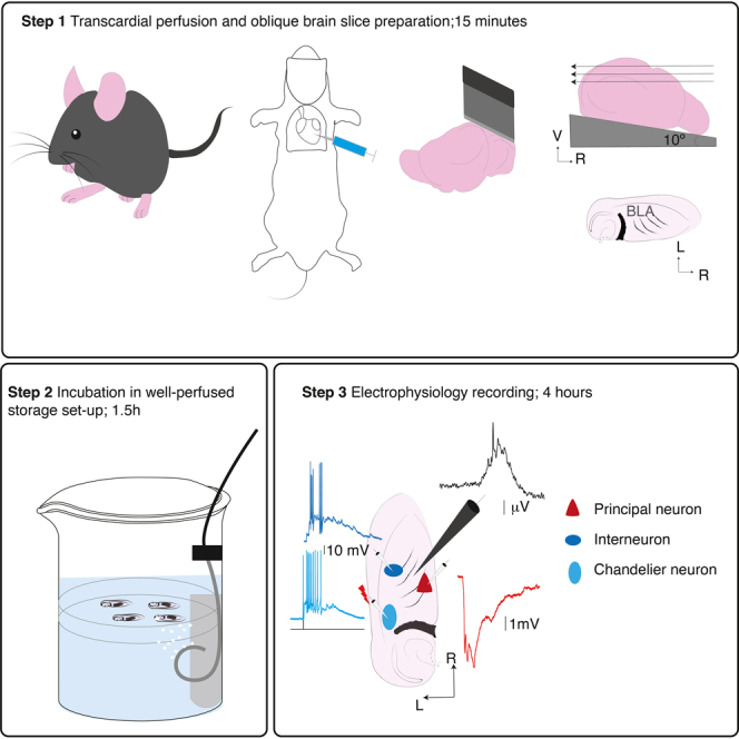
On the day of experiment, freshly prepare extracellular solution. Cool cutting solution and prepare set up for dissection. Take 300 mL of cutting ACSF solution and saturate with carbogen by bubbling for ∼30 min before cooling the solution to ice cold. After bubbling for ∼30 min, we cooled the solution rapidly by keeping it in −80°C for ∼ 20 min. Continuously bubble the solution with carbogen during dissection and slice preparation. This step involves anaesthetizing a rat or mouse for trans-cardial perfusion with ice-cold carbogenated cutting solution, extracting the brain, and obtaining oblique horizontal slices containing BLA using a vibratome. Slices are stored in normal extracellular solution in an in-house designed storage chamber at 37°C for ∼120 min and then at room temperature ∼ 24°C. In our experience, trans-cardial perfusion significantly improved viability of slices obtained from 3–12 weeks old adult mice and 3–8 weeks old rats. Typically, it takes ∼15–20 min from anesthetizing animal to obtaining slices.

• 1.
  Before starting slice preparation:

  • a.
    Ensure all equipment necessary for trans-cardial preparation and dissection are ready and organized for quick access. Tools: 21 Gauge needle connected to short tubing (∼5 cm) and other end attached to a three-way stopcock, 2× 20 mL syringes, general dissection tools such as a small and large operating scissors, spatulas, forceps, single edged blade, beakers, petri-dishes, filter paper, a super glue tube that can dry quickly, inhouse-made 10° block or flat plate to glue the brain and the slicing chamber.
  • b.
    Clean a razor blade with 70% ethanol and rinse with deionized water thoroughly. Fit the blade to the blade holder in the vibratome.
• 2.
  Incubation set up:

  • a.
    Design a storage chamber using a 460 mL beaker, petri-dish- bottom replaced with a nylon mesh (we used commercially available stocking material) and Tygon tubing connected to carbogen source (Figure 1A).
  • b.
    Arrange the tube to form a C-shape and with pores along the upper curvature.
  • c.
    Make pores using patch electrode pipettes. This chamber is filled with extracellular solution ∼250 mL and continuously bubbled with carbogen.

Note: This arrangement for carbogen delivery facilitated extracellular solution to circulate continuously around the slices placed on the nylon mesh. Typically, slices are submerged ∼ 12 mm under the circulating extracellular solution.

CRITICAL: The storage chamber with solution should be pre-warmed to 37°C before slice preparation.

• 3.Animals: rats or mice.

CRITICAL: All animal experiments must comply with national and institutional ethics approval.

• 4.
  Preparing oblique brain slices containing BLA.

  • a.
    Before anesthetizing the animal, load two 20 mL syringes with ice-cold and carbogenated cutting solution, connect them to the stopcock for transcardial perfusion and set it ready for perfusion. Make a soft bed with tissue paper in a large square weighing boat. Place the weighing boat on a thick thermocool sheet.
  • b.
    Anesthetize the animal using isoflurane sealed plexiglass container placed in a fume hood. Once the animal breathing has slowed down, pinch the paw for any pain response. If the animal is unresponsive, remove animal from the container. Insert the head inside a falcon tube containing cotton balls dabbed with isoflurane. Place animal on its back on the tissue bed in the weighing boat. Pin the front paw if required.
  • c.
    Lift the abdominal skin with forceps and use scissors to cut open the thorax. Cut the diaphragm carefully to expose the heart. Puncture the right atrium, then puncture the left ventricle with the 21G needle to perfuse ∼40 mL of ice-cold cutting solution. After perfusion, decapitate the mouse with large scissors. For rats, a rodent guillotine is used to decapitate. Place the head in a petri-dish with ice-cold cutting solution.
  • d.
    Open the skull using cuts on the left and front or through midline and front. Care must be taken not to damage the brain. Remove the brain using a small spatula into a small beaker or petri-dish filled with ice-cold cutting solution and bubble with carbogen.
  • e.
    Oblique horizontal brain slice preparation. Place the ventral side of the brain on a filter paper moistened with cutting solution on a flat surface (petri dish or a glass plate). Using a single edge blade cut and remove the cerebellum. Lift the brain from the filter paper using a small filter paper or spatula. Gently dry the dorsal surface of the brain and glue it to the slicing block ∼10° (Figure 1B) and quickly place it in a slicing chamber, fill with ice cold cutting solution and bubble with carbogen. Alternatively, to obtain the same angle, use a single edged blade to make a cut tangential to the dorsal cerebrum ∼10° and glue the cut surface to a flat plate. In both cases, the rostral end is in the downhill position (Figure 1B).The BLA lies ∼500 μm and ∼700 μm from ventral surface in mouse and rat brain, respectively.
  • f.
    The first 2 slices from either side are typically discarded. Slices containing BLA as a triangular region (Figure 1C) can be identified by landmarks such as the external capsule on the lateral side and hippocampus in the caudal end. We cut 400 μm thick horizontal slices and usually 4 slices (2 from each side) contain the BLA. Transfer slices to the storage chamber filled with circulating pre-warmed external solution. Slices are incubated for ∼120 min at physiological temperature (∼37°C) and subsequently stored at room temperature (24°C–26°C).

CRITICAL: (1) Cutting solution should be saturated with carbogen and kept ice-cold throughout slice preparation. (2) Limiting the duration of slice preparation within 20 min helps to obtain good quality slices.

Note: (1) In our experience, slices from 275 μm thickness showed SWs. However, we recommend 400 μm thick slices for stable local field potential recording. (2) We used either in-house made metal block or tangential cut on the dorsal side of cerebrum to obtain oblique slices and both methods reliably had network activity. Alternatively, make an agar block (see below for making 4% agarose solution) with desired angle to make oblique slices. (3) In our experience, circulation of carbogenated extracellular solution during incubation and storage is critical for the emergence of network activity. In our set-up, slices were kept submerged at ∼ 12 mm from the surface of ACSF. Limiting this volume can allow exchange of ACSF and better perfusion of slices. Alternatively, commercially available storage chambers such as Haas-type interface chambers provide continuous perfusion to slices and are used to record network activity in the hippocampus ex vivo (Maier et al., 2009). (4) We incubated slices at 37°C for the recovery of ion channels and pumps at physiological temperature. In our experience, incubation at this temperature reliably showed SWs. However, other studies have used ∼33°C (Maier et al., 2009) incubation in interface-type chambers for 2 h and observed SWs in hippocampus. (5) Large temperature changes from storage to recording chamber also can affect stability of network activity. We transferred one slice at a time after 2 h incubation at 37°C. Slices transferred within 1 hour (usually first 2 slices) after incubation at 33°C and subsequent slices at 28°C–30°C.

Figure 1.

Preparation of oblique slices containing basolateral amygdala (BLA) and recording for spontaneous sharp-wave ripples

(A) Photo of in-house designed storage chamber filled with extracellular solution and bubbled with carbogen delivered through a curved tubing.

(B) Schematic of brain glued on its dorsal side on an angled block (10°) and dotted arrows indicate slicing blade movement. Schematic below shows a typical oblique horizonal slice and and boundaries of the BLA highlighted as a triangular region highlighted in red.

(C) Top photo of 5× image shows a typical oblique horizontal slice containing BLA. Photo below shows BLA as a triangular region bounded laterally by external capsule and caudally by hippocampus. Scale bar: 100 μm. Inset below shows a representative 20× image of viable BLA neurons. Note the smooth appearance of somata. Scale bar: 50 μm.

(D) PNs and INs can be distinguished from intrinsic action potential (AP) discharge characteristics. Top, representative traces from a PN (red) and an IN (blue) showing regular and fast continuous discharge patterns. Bottom left, superimposed APs recorded in a PN (red) and IN (blue) showing that the PN-AP is wider; right, the width at the half-maximal amplitude of AP (AP half-width) in PNs (0.9 ± 2 ms, n=72) was significantly wider than in INs (0.4 ± 0.1 ms, n=54, t-test with Welch correction, p-value < 0.0001).

(E) Spontaneous LFP recording in the BLA. Representative image shows extracellular electrode placed in the BLA to record LFP, scale bar: 100 μm. Top trace shows spontaneously occurring deflections in the field potential. Same LFP signal filtered for sharp-wave (1–20 Hz) and ripple (100–300 Hz, bottom) frequencies. Note that each filed potential deflection contain both SW and ripple frequencies.

(F) Simultaneous recording for field potential and correlated post-synaptic potentials in a PN (red triangle) and an IN(blue oval). Top trace show LFP signal filtered for ripple frequency band that occur concurrently with inhibitory post-synaptic potentials (IPSPs) in the PN and excitatory post-synaptic potentials (EPSPs) with a burst of action potentials in the IN.

(G) LFP and same pair of cells in voltage clamp showing ripple-associated inhibitory post-synaptic currents (IPSC) in the PN (Vh −50 mV; middle) and excitatory post-synaptic currents (EPSC) in the IN going (Vh −70 mV, bottom). Data reported already in Perumal et al. (2021).

Electrophysiology

Timing: ∼4 h

The main goal of the experiment is to obtain extracellular local field potential (LFP) recording in the BLA and simultaneously record from neuronal subtypes to elucidate their engagement with the network activity. After incubation, slices are transferred one at a time to the recording chamber perfused with pre-warmed and carbogenated extracellular solution and visualized under an upright microscope, either an (1) Olympus-BX50WI fitted with Infrared differential interference contrast, 40× water immersion objective and a fluorescent lamp (Olympus U RFLT, Olympus Optical) or (2) an Axio Examiner Z1 fitted with Dodt gradient contrast, 5× and water immersion objectives 40× (Zeiss, Germany) or 60× (Olympus) and a fluorescent lamp (X-cite 120Q, Excelitas) and a video camera either IR-1000 (Dagemti, USA), ProgRes (Jenoptik, Germany) or Retiga Electro (QImaging, Canada). Electrical signals were acquired with a Multiclamp 700A and 700B amplifier (Molecular Devices, USA), digitized using ITC-16 A/D converter (InstruTECH, Germany), and recorded using Axograph X (Axograph Scientific, USA). Amplifier head stages were mounted on Patch-star manipulators (Scientifica, UK). The local field potential (LFP) generated by the network activity was recorded using a low-resistance extracellular patch electrode filled with 150 mM NaCl or external solution. The LFP signals from extracellular field electrodes are acquired with a Bessel filter set at 1 Hz–1 KHz and digitized at 50 kHz with x2000 amplification. For the LFP signal, the mains interference (50 Hz) was removed using Humbug (Digitimer, UK). For intracellular recordings, electrical signals are acquired from DC −10 kHz and digitized at 50 kHz. Start the electrophysiology set up at least 30 min prior to the start of the experiment.

• 5.
  Setup and preparation before recording

  • a.
    We used a submerged type recording chamber perfused with pre-warmed carbogenated external solution at 5–7 mL/min (33°C–34°C or 28°C–30°C). High perfusion rate is key for maintaining network activity in the recording chamber due to high metabolic demand. Keep the bath volume as low as possible to reduce pipette capacitance.
  • b.
    Take an aliquot of intracellular recording solution and thaw under room temperature ∼30 min before recording. We routinely added biocytin (∼0.3%) to whole-cell patch clamp solution. Biocytin can be added while preparing internal solution. However, it is preferable to add fresh before start of experiment. After adding biocytin, sonicate for ∼5 min until solution is clear. Patch pipette fillers can be custom made from plastic pipette tips (200 μL, yellow) with gentle heat and stretching to form a thin tube. This pipette filler is then connected to a 0.22μm filter unit (pipette filler unit). Load intracellular solution in a 1 mL insulin injection syringe and connected to the pipette filter unit.
  • c.
    Make a second pipette filler unit. Fill a 1mL insulin injection syringe with 150 mM NaCl or external perfusion solution and connect it to the filler unit.
  • d.
    Pull glass pipettes for extracellular and whole-cell patch recording electrodes. Borosilicate glass capillaries are pulled using a vertical puller (PC 10 dual stage puller, Narishige). Pull extracellular glass electrodes using Borosilicate glass capillaries and adjust heat settings to get tip resistance of 1–2 MΩ. Whole-cell patch clamp electrodes had tip resistance of 4–6 MΩ.
  • e.
    Transfer one slice at a time to the recording chamber and secure it using a ‘U’ shaped harp with nylon strings. Visualize the slice under 5×. In oblique horizontal slices, the BLA can be distinguished as a triangular region demarcated medially and laterally by fiber bundles, and caudally by the lateral ventricle and hippocampus (Figure 1C).
  • f.
    Under 40× or 60× objective visualize the quality of slice. Adjust optics for visualizing somata coming above the surface. Healthy somata show a smooth surface and opaque (typically nucleus not visible). Healthy slices typically show many such cells (Figure 1C bottom) and critical for network activity.
  • g.
    Fill an extracellular glass electrode with 150 mM NaCl or external perfusion solution and mount the electrode to pipette holder. Apply a small positive pressure while lowering the electrode tip to the surface of the slice. Maintain positive pressure and gently lower the tip into the slice until the pipette tip is buried into the slice. Release the pressure and the tissue wraps around the pipette tip. In current clamp configuration (with settings for LFP), monitor field potential deflections. It takes ∼1–3 min tissue around the pipette tip to settle and stabilize field potential baseline. Monitor for deflections in LFP signal for a sharp upward or downward going epochs lasting ∼ 50 ms that occur at ∼30 events/min (Figure 1E).

Note: Keep the bath volume as low as possible to enhance perfusion of slice for network activity and reduce pipette capacitance for intracellular recordings. Alternatively, an interface like chamber or submerged chamber with dual perfusion setups can be used to maintain network activity (Maier et al., 2009). Since BLA has a non-laminar cellular organization, unlike the hippocampus, SW LFP signal amplitudes are small and can occur as upward or downward deflections. In our experience, placement of the extracellular electrode in lateral part of BLA yielded best results (as in Figure 1E), but reliable recordings can be obtained throughout BLA as SWs are generated by population burst activity. We suspected pipettes filled with external solution may develop microscopic precipitates over time (due to lack of carbogen) that may affect the recordings. As an alternative, we used 150 mM NaCl as LFP electrode filling solution. However, both methods yielded similar results within the recording duration. LFP signal to noise ratio can be improved by using 0.5–1 M NaCl as electrode filling solution in patch recording electrode. High molar salt solution reduces electrical resistance significantly, however, care should be taken as leakage of this solution into the tissue will affect the slice viability and cells in the vicinity of the electrode tip. It is ideal to place the extracellular electrode first before obtaining intracellular recordings. Usually, whole-cell patch clamp recordings were obtained from neurons >100 μm away from the LFP electrode.

• 6.
  Dual SW LFP and whole-cell patch clamp recording to identify cellular correlates of network activity: To obtain dual recordings, it is essential to check that electrophysiology rig, manipulators and head-stages are set up to minimize transfer of vibration.

  • a.
    Under 40× or 60× magnification and DIC/Dodt contrast look for smooth healthy cells. Fill a pulled patch glass electrode with intracellular solution. Apply small positive pressure (∼20 mbar) and bring the tip close to soma. Press the tip gently on the soma and observe for a dimple. Release positive pressure and apply a gentle and subtle negative pressure or voltage (-70 mV) to help the seal, wait unit seal resistance exceeds at least one giga ohm, and release positive pressure to form tight seal (>1.5 GOhm seal). Apply a short pulse of gentle suction to break into whole cell configuration. Gently blow out membrane debris out of the pipette to improve access resistance of the whole-cell configuration. Switch to current clamp configuration and measure resting membrane potential (typically <-60 mV). If the resting membrane potential is more depolarized (>-50 mV), lose the recording and pick another cell. In slices obtained from transgenic mice lines, interneurons can be visualized using fluorescent light excitation. Keep fluorescent light exposure minimal to reduce photo-toxicity and bleaching. Identify a fluorescent soma and switch to DIC/Dodt mode to visualize. Verify if the somatic membrane is healthy looking and use same steps as above to obtain whole-cell patch recording. The same steps can also be followed to obtain simultaneous recordings from two neurons along with LFP. PNs and INs can be distinguished by their intrinsic electrophysiological properties (Figure 1D). Using a small step current injection (first step -50 pA, increment by 30 pA, 600 ms). PNs discharge at much lower frequency with wider action potentials than INs (Figure 1D). For more details, please refer to Perumal et al. (2021).
  • b.
    SW associated intra-cellular correlates: Upon conversion to whole-cell configuration monitor online for spontaneously occurring epochs of large post-synaptic potentials (PSP, current clamp) or post-synaptic currents (PSC, voltage clamp). SW- correlated events occur time-locked with every LFP deflection and are large multi-synaptic inputs as compared to mono-synaptic inputs to the same cells and can be detected online. Secondly, PNs and INs receive distinctive SW associated inputs.
  • c.
    SW associated PSPs: Switch to current clamp configuration and record spontaneous SW associated PSPs for at least 3 min. In PNs, SW-PSPs occur as depolarizing potentials from rest (∼-70 mV) but reverse polarity at ∼ −60 mV, hyperpolarizing the cell. In current clamp, inject positive current to depolarize membrane potential to ∼-50 mV and record spontaneous SWi-PSPs which occur as long-lasting hyperpolarizing PSPs (Figure 1F). Record reversal polarity of SW-PSPs by setting membrane potential from −80 mV to −50 mV (see Figure 1E in Perumal et al., 2021).
  • d.
    Using fluorescence guidance, obtain whole cell recording in an IN. In INs, SW-PSPs occur as excitatory potentials triggering a burst of action potentials.
  • e.
    SW-PSPs in PNs and INs occur simultaneously with SW-LFP. Obtain dual recording using the same steps as above and monitor for spontaneously occurring SW-PSPs. SW-PSPs occur simultaneously (±30 ms) between neurons within BLA.
  • f.
    SW associated PSCs: Switch to voltage clamp configuration to record SW-PSCs. In PNs, set holding potential to −70 mV and monitor for SW-PSCs which occur as large inward currents time-locked with LFP deflections. Change the holding potential to −50 mV and monitor for SW-PSCs. Notice SW-PSCs occur as outward currents (Figure 1G). Set holding potential from −80 mV to −50 mV to record reversal of SW-PSCs. Due to GABAergic origin of SW inputs to PNs, SW-PSP/PSCs reverse polarity near −60 mV, near Cl^- reversal for whole-cell recording solution (see Figure S1H in Perumal et al., 2021). In interneurons, set holding potential to −70 mV and monitor epochs of large inward currents. It is noteworthy that SW-PSCs in PNs and INs display consistent waveform between episodes, cells and slices. For detailed description of SW-PSC waveform please refer to (Perumal et al., 2021).
  • g.
    SWs and associated intracellular events show dual pharmacological sensitivity to antagonists for GABA_A and AMPA receptors. Perfuse antagonists for GABA_A and AMPA receptors sequentially to verify dual sensitivity (see Figure 1K in Perumal et al., 2021). We used following GABA_A receptor antagonists: Bicuculline (10 μM), Gabazine (3 μM), and Picrotoxin (100 μM) and AMPA receptor antagonists: 2,3-Dioxo-6-nitro-1,2,3,4-tetrahydrobenzo [f] quinoxaline-7-sulfonamide (NBQX, 10 μM) and 6-Cyano-7-nitroquinoxaline-2,3-dione (CNQX, 10 μM).

Note: (1) SW associated intracellular events (SWi) have consistent waveform and synaptic properties in BLA neurons (Perumal et al., 2021). In addition to LFP, SW-PSPs and PSCs are a reliable proxy to detect network activity in the slice.

• 7.
  Targeted recording from INs initiating SWs in the BLA: In the BLA, SWs and associated synaptic events can be initiated by a rare subset parvalbumin (PV) expressing GABAergic neurons, chandelier interneurons, that make synaptic contacts at the axon initial segment (AIS) of postsynaptic PNs. Individual BLA chandelier INs contact ∼200 PNs forming characteristic cartridge synapses at the AIS, the site of action potential initiation. To our knowledge, molecular markers exclusively targeting chandelier INs are unavailable for BLA. Even among PV INs, chandelier INs make a small proportion of (<10 %). Further, similar to basket PV INs (90% of PV INs) chandelier INs display fast spike discharge with depolarizing current injections. Thus, obtaining targeted recording from chandelier INs remains a challenge. Our group and others have reported that chandelier INs evoke a characteristic time-locked feedback excitation(Molnar et al., 2008; Perumal et al., 2021; Spampanato et al., 2016; Szabadics et al., 2006; Taniguchi et al., 2013; Woodruff et al., 2006). This evoked feedback excitation occurs exclusively in chandelier INs and suggests this feeback excitation as an electrophysiological marker(Woodruff and Yuste, 2008). Using a combination of somato-dendritic features and evoked feedback excitation enhanced our success rate to encounter chandelier INs. In the BLA, we predominantly encountered these cells in the lateral and caudal BLA (Figure 2A).

  • a.
    Under a 40× objective, visualize INs using fluorescence guidance. Adjust exposure and gain settings on the video acquisition software to visualize somata and proximal dendrites. Look for somata with square or triangular shape that also have a thick bifurcating dendrite at one corner (Figure 2A).
  • b.
    Once a suitable IN soma is identified, switch to DIC/Dodt contrast mode and verify health of the neuron to obtain whole-cell patch clamp recording.
  • c.
    Obtain whole-cell recording using step 6a and monitor for spontaneous SW associated synaptic PSPs in current clamp.
  • d.
    In current clamp, inject depolarizing current steps to elicit intrinsic discharge properties. Ins fire narrower action potentials than PNs and also discharge at high frequency with distinctive firing patterns (Figure 2B) (Woodruff and Sah, 2007; Perumal et al., 2021). In our experience, Ins with feedback excitation showed 4 types of fast spiking discharge patterns characteristic of PV subset of Ins (Figure 2C).
  • e.
    Monitoring for evoked feedback excitation: In current clamp, use square current pulse 1–2.5 nA for 0.5–1 ms to evoke a single action potential. Monitor for a EPSP or EPSP burst immediately after the action potential. Run this protocol for 30 or more trials (preferably 100 trials). Presence of feedback excitation can be detected online by occurrence of an EPSP immediately after the action potential (Figure 2D). This evoked feedback EPSP occurs time-locked at ∼ 2–4 ms, with at high success rate (∼ 83%). The latency of the feedback EPSP indicates it originated from a di-synaptic circuit. Notice that same cells can also evoke multi-synaptic burst of SW associated EPSPs (40±26% trials) which typically triggers time-locked action potentials riding on time-locked EPSPs (Figure 2D).
  • f.
    Monitoring for feedback excitation in voltage clamp: Switch to voltage clamp and set holding potential to −70 mV. Apply a square pulse of +70 mV for 0.5 ms. This pulse evokes a single unclamped ‘action current’. Monitor online for an inward current immediately following ‘action potential’ current (Figure 2E). Like in current clamp, this presence of di-synaptic feedback can be detected online as it occurs time-locked at ∼2–4 ms following voltage step. Notably, a single discharge in these cells is sufficient to trigger successive waves of SW-EPSCs at regular intervals of ∼ 4 ms and they consistently summate within ∼20 ms.
  • g.
    Chandelier Ins evoked feedback excitation shows dual pharmacological sensitivity to GABA_A and AMPA receptor antagonists (Figure 2E). Bath apply antagonists for AMPA and GABA_A receptors sequentially to verify dual sensitivity.
  • h.
    After recording, slices are transferred to fixative for the recovery of morphology and verification of axo-axonic synaptic contacts.

Note: (1) In the BLA, chandelier Ins are frequently encountered at the lateral and ventral regions and typically show fast-spiking characteristics of PV-Ins. (2) Soma and dendritic morphological features described here is only a guidance. In our experience, these criteria enhanced recording neurons with feedback excitation in 1 out of 4 cells. (3) IN discharge evoked SW-burst involves multi-synaptic recruitment of other neurons, thus depends on intact connections in the slice. We encountered 19/102 cells with di-synaptic feedback excitation that also evoked SW burst.

Figure 2.

Targeted recording from GABAergic interneurons (INs) initiating SW burst

(A) Left, photo of oblique brain slice and dots (cyan) indicate approximate location of INs that evoked feedback excitation. Scale bar: 100 μm. Right, top and bottom photos show of triangular and square shaped somata of INs with feedback excitation. Red arrowhead indicates thick bifurcating dendrite. Scale bar:10 μm.

(B) Traces show four types of intrinsic action potential discharge patterns elicited by depolarizing suprathreshold current injection in INs with feedback excitation.

(C) Top, somata shape among recovered INs with feedback excitation. Bottom, proportion of cells with distinct intrinsic discharge patterns.

(D) Whole-cell recording from a fast spiking IN. An action potential evoked with depolarizing current injection (1.5 nA, 1 ms) evoked a time-locked di-synaptic feedback EPSP (red arrow); inset shows mean trace of feedback EPSPs (cyan) overlaid on individual trials. Bottom traces show trials when the action potential evoked a summating EPSP burst, driving time-locked action potentials; a single trial highlighted in cyan is overlaid on individual trials.

(E) Voltage-clamp recording (Vh −70 mV) in the IN. A depolarizing voltage step (+70 mV, 0.5 ms) evokes an unclamped 'action potential current' followed by a time-locked burst of feedback excitatory postsynaptic currents (EPSCs, red arrow). The mean trace in cyan overlaid with individual trials. Bottom graph shows distribution of EPSCs in all trials (n=40 trials). Note regular spikes at intervals ∼4 ms following the evoked action potential current at 0 ms. The di-synaptic feedback is highlighted by dotted rectangle.

(F) The evoked feedback burst was reversibly blocked by a AMPA receptor antagonist, CNQX (upper) and a GABA_A receptor antagonist, gabazine (lower). Data reported in Perumal et al. (2021).

Immunohistochemistry

• 8.
  Prepare solutions for immunolabeling

  • a.
    Prepare fixative: 200 mL of 4% Paraformaldehyde in 1× Phosphate Buffered Saline (PBS), pH ∼7.4, store at 4°C and use within 5 days.
  • b.
    Blocking solution: 0.5% Bovine Serum Albumin (BSA) and 0.05% Saponin in 1× PBS. Blocking solution can be prepared as 20× stock, stored in 1mL aliquots in −30°C and used in ∼8 weeks.
  • c.
    Sodium azide stock: Make 10% sodium azide stock solution in dH2O. To prevent microbial growth, add sodium azide (0.05%) to blocking solution.
  • d.
    4% Agarose in H₂O is used to embed slices and sub-sectioned to label for synaptic contacts.
• 9.
  After whole-cell patch recording, neurons can be recovered for morphology by immunolabeling for biocytin. Interneurons in the BLA have a dense axonal plexus. For morphological recovery, it is best to limit number of sampled Ins to one or two to avoid overalap of axonal arbors. Solutions for immunolabeling are prepared prior to preparing for electrophysiology. A detailed immunolabeling protocol is beyond the scope of the article. For more details, please refer to https://theolb.readthedocs.io/en/latest/index.html.

  • a.
    After whole-cell patch recording (typically lasts at least ∼30 min) transfer the slice to a 16 well plate filled with fixative and incubate for ∼1 h at room temperature inside a hood for rapid fixation.
  • b.
    At the end of experiments, transfer slices in the fixative for overnight (∼12 h) incubation at 4°C.
  • c.
    Following day, slices are resuspended in PBS and rinsed for 3 × 15 min.
  • d.
    Resuspend the slices in blocking buffer and incubated on a shaker for 1 h at room temperature.
  • e.
    Recovery for biocytin. Add Alexa Fluor −555 bound to streptavidin (1:2000, Invitrogen) and incubate 24 h at room temperature.
  • f.
    On the following day, remove the blocking buffer and resuspend slices in PBS, wash for 3× for 15 min each.
  • g.
    Mount the slice on a glass slide with DABCO to preserve fluorescence labeling. A glass cover slip is placed on top of the slice and held in position by sealing the sides with nail polish. Cover the slides from light and allow the polish to dry and seal.
  • h.
    Verify immunolabeled neurons using an upright fluorescence microscope (Axio Imager, Zeiss). For detailed morphological characterization, we imaged neurons with a spinning-disk confocal system (Marianas; 3I, Inc.) consisting of a Axio Observer Z1 (Carl Zeiss) equipped with a CSU-W1 spinning-disk head (Yokogawa Corporation of America), ORCA-Flash4.0 v2 CMOS camera (Hamamatsu Photonics), 20× 0.8 NA PlanApo and 40× 1.2 NA C-Apo objectives. Image acquisition was performed using SlideBook 6.0 (3I, Inc). Morphological reconstruction was carried out manually using Neurolucida-360 (MBF Bioscience) and visualized in NeuroExplorer (MBF Bioscience).
• 10.
  After imaging, embed slices in 4% agarose for sub-sectioning. For this step, prepare other tools such as a dedicated vibratome for immunohistochemistry, single edged blade, a paint brush, glass petri-dish etc. For more details, please refer to https://theolb.readthedocs.io/en/latest/index.html.

  • a.
    Using a large petri-dish that can fit the length of the glass and fill with 1× PBS.
  • b.
    Place glass slides with slices in the petri-dish. Using a single edged blade cut through the sealed sides of the cover slip.
  • c.
    Using a paint brush gently move the cover slip and allow the slice to be completely dislodged from the slide.
  • d.
    Transfer the slice into a 16-well plate filled with 1× PBS.
  • e.
    Gently warm 4% agarose in a microwave for ∼2–3 min and stir to ensure solution is clear without precipitates. If overheated, the solution turns yellow and may not embed slices well. In this case, discard and make a new batch.
  • f.
    Transfer a slice on to a glass slide or small glass petri-dish. Gently remove excess PBS as much as possible using a filter paper without touching the slice. This is critical for proper embedding.
  • g.
    As quickly as possible transfer a large drop of agarose solution (∼40°C) on the slice and wait for agar to solidify at room temperature (∼25°C).
  • h.
    Once solidified, trim the excess agar.
  • i.
    Transfer embedded slice block to a dedicated vibratome (VT1000S vibratome, Leica) exclusively for immunohistochemistry and cut to 70 microns thick slabs submerged in 1× PBS.
  • j.
    Suspend sub-sectioned slices in the blocking buffer as described above.
  • k.
    Add primary antibodies labeling for parvalbumin (mouse anti-parvalbumin, 1:2000, Sigma-Aldrich) and Ankyrin-G (rabbit anti-Ankyrin G, 1:500, Santa Cruz) and incubate at room temperature for two days.
  • l.
    After two days, gently remove blocking buffer and wash slices with 1× PBS, 3 times for 15 min each.
  • m.
    Remove PBS and add blocking buffer containing secondary antibodies conjugated with fluorophores: goat anti-mouse, Alexa 405 (1:1000, Life Technologies) and goat anti-rabbit, Alexa Fluor 647(1:1000, Invitrogen).
  • n.
    Incubate for 1 day at room temperature.
  • o.
    On the following day, remove blocking buffer and wash slices 3× with 1× PBS, for 15 min.
  • p.
    Mount slices on glass slides with DABCO. We imaged synaptic contacts with 63× and 100× oil immersion objectives and imaged with spinning-disk set-up described above.

Expected outcomes

Using the slice preparation method described in steps 1–4 will yield high quality slices from adult animals with viable neurons (Figure 1C) and generating spontaneous network activity (Figures 1E and 1F). Protocol described in step 5g is expected to provide optimal method to get stable LFP recordings (Figure 1E), however, some optimization may be required to achieve consistent recordings. Health of neurons is crucial to obtain high resolution whole-cell recordings (Figure 1F). Protocol described in step 7 will guide selections interneurons initiating the network activity (Figures 2A and 2D). In our experience, patience in selecting cells is key to yield best results. Stable whole-cell recordings for at least 30 min will allow diffusion of biocytin to fine processes such as the axons (Figure 3A) and recovery for immunolabeling for synaptic contacts (Figure 3B).

Figure 3.

Axonal arborization and synaptic targeting of chandelier INs in the basolateral amygdala (BLA)

(A) Extensive axonal arborization by INs with feedback excitation in the BLA. Reconstruction of three INs (top and bottom left) that evoked feedback excitation with soma and dendrite in blue and axon in red. Same three cells overlaid on a mouse BLA slice with their approximate location. Note individual neurons cover extensive area of BLA. Scale bar: 100 μm.

(B) The axonal plexus of INs with feedback contained strings of synaptic bouton ‘‘cartridges’’ in close approximation to the axon initial segment marker Ankyrin G. Top panel, 20× magnified image of recovered axonal plexus from an IN with feedback burst showing multiple strings of synaptic bouton cartridges (red arrows); the inset shows a 100× magnification of a cartridge containing a string of synaptic boutons (red arrows). Bottom panels from the same axon at 100× magnification and panels from left to right show two axon initial segments stained for Ankyrin G (white), biocytin-recovered cartridge synaptic boutons in the same location, and superimposed images of biocytin and Ankyrin G staining exhibits close approximation of cartridge synaptic boutons (red) on Ankyrin G (white). Scale bar: 10 μm. Data reported already in Perumal et al. (2021).

Quantification and statistical analysis

For quantification and data analysis of SWs and SW intracellular events, please refer to (Perumal et al., 2021). As described above, network activity associated events can be readily detected online while recording. Here we describe main quantification methods used to analysis LFP and intracellular synaptic events.

LFP analysis for SWs and ripples: LFP deflection can be detected and aligned to peak using amplitude criteria in Axograph. Capture detected events ± 400 ms from the peak with and verify manually and export to MATLAB for generating spectrograms. Alternatively, wide-band LFP signal can be band-pass filtered between 1-20 Hz for SWs and 100–300 Hz for ripples.

SW associated synaptic events: SW-associated intracellular post-synaptic potentials/currents (SWi PSPs/PSCs) are many-fold larger than mono-synaptic events both in amplitude and duration. Capture SWi using amplitude threshold (in-built event detection function in Axograph) and verify visually. Captured episodes with a data window of ± 400 ms aligned to the peak. Analyze temporal structure of captured SWi-PSCs for intrinsic frequency and summation window. Captured episodes then exported to MATLAB for generating spectrograms (see Figure 1J in Perumal et al., 2021). The time to reach peak amplitude was calculated as the difference between the onset and location of the peak amplitude for each episode.

Analysis for IN evoked feedback excitation: IN evoked feedback excitation is analyzed for success rate, timing of the peak amplitude for each EPSC burst and peak amplitude. Both SW-EPSCs, evoked feedback EPSC burst shows spectral power in same frequency bands and time to peak (Figure 2e in Perumal et al., 2021).

Limitations

Successful patch clamp recordings require preparation of viable slices, optimal visualization settings and stable electrophysiological set up. Good quality slice preparation needs rigorous maintenance of equipment, storage containers and tools. After dissection, we thoroughly rinse and clean all equipment and spray with 70% ethanol to decontaminate. Storage chamber needs to be sprayed with 70% ethanol and then thoroughly rinsed under deionized water for at least 15–30 min. Preparing oblique slices may require optimization as brain size and shape can vary between animal strains. Incubation in a well-perfused storage chambers also key to observe network activity in slices.

Fluorescence in slices obtained from transgenic mice line provide useful method to target INs. However, fluorescence loss due to long exposure and with time is inevitable. Limiting exposure of slices to white light during storage such as by shielding with foil can help to reduce loss of fluorescence. It is important to optimize camera settings to get best fluorescent and contrast image with limited exposure.

Axons of individual INs densely innervate BLA (Figure 3). For morphological recovery and staining for synaptic contacts, it is best to limit number of cells sampled in each slice to minimum (∼2) and far apart from each other.

Troubleshooting

Problem 1

Slice viability for electrophysiology recordings (steps 1–4 in acute brain slice preparation).

Potential solutions

Slice preparation is the key step to get successful and stable recordings. It is critical that all tools used for dissection should be cleaned thoroughly after use and free of any harmful chemicals. Dissection tools used for electrophysiology should be kept separate and not used for other purposes (such as dissections using fixatives). All beakers and containers should be cleaned thoroughly for any contamination or residual salts. Trans-cardial perfusion enhances slice viability, however, requires experience to complete the procedure quickly to get best results. Solutions should have correct composition to get correct osmolarity and pH. Intracellular solution should have correct osmolarity to get giga ohm seal and stable whole-cell recording. Further, regular maintenance of patch electrode holder for salt deposits, leakage, and regularly coating the silver wire helps to achieve stable and good quality recordings.

Problem 2

Local field potential recordings (step 5g in electrophysiological recording).

Potential solutions

Recording LFP in the BLA is a challenge and requires optimizing pipette tip size, shape, and placement to get stable recordings and detect SWs online. If LFP detection is difficult, first verify for network activity with intracellular correlate using whole-cell patch recording. Using 0.5 or 1 M NaCl as filling solution for extracellular electrode will greatly reduce access resistance, but slice quality may deteriorate due to leakage of pipette solution into the tissue.

Problem 3

Targeted recording from interneurons (step 6a in electrophysiological recording).

Potential solution

Optimizing fluorescence imaging is important to get targeted recordings from interneurons using transgenic mouse lines. Particularly, it is a key step to search for cells with specific soma and dendritic morphology before losing fluorescence.

Problem 4

Multi-cellular recording (step 6a in electrophysiological recording).

Potential solution

For successful multicellular recording, it is crucial that electrophysiology set up is placed on air table to reduce vibration that can affect patch electrodes. Head-stages on the manipulators should be fixed firmly, aligned for changing electrodes without colliding with the other electrodes, and isolated for transfer of vibration between electrodes.

Problem 5

Recovering axonal processes for synaptic contacts (steps 7 and 8 in immunohistochemistry).

Potential solution

Typically, whole-cell patch clamp recordings last at least ∼30 min. During this time, biocytin in the intracellular recording solution diffuse enough to recover axons. It is best to use freshly prepared PFA to fix slices. IN axons form dense and extensive plexus in the BLA. It is best to limit number of cells to a minimum as possible.

Resource availability

Lead contact

Further information and requests for resources and reagents should be directed to and will be fulfilled by the lead contact, Pankaj Sah (pankaj.sah@uq.edu.au).

Materials availability

This study did not generate any unique reagents

Data and code availability

Original source data for Figures are available in the main text or the supplementary materials of Perumal et al. (2021).

References

- Bahner F., Weiss E.K., Birke G., Maier N., Schmitz D., Rudolph U., Frotscher M., Traub R.D., Both M., Draguhn A. Cellular correlate of assembly formation in oscillating hippocampal networks in vitro. Proc. Natl. Acad. Sci. U S A. 2011;108:E607–E616. doi: 10.1073/pnas.1103546108. [DOI] [PMC free article] [PubMed] [Google Scholar]
- Maier N., Morris G., Johenning F.W., Schmitz D. An approach for reliably investigating hippocampal sharp wave-ripples in vitro. PLoS ONE. 2009;4:e6925. doi: 10.1371/journal.pone.0006925. [DOI] [PMC free article] [PubMed] [Google Scholar]
- Maier N., Nimmrich V., Draguhn A. Cellular and network mechanisms underlying spontaneous sharp wave-ripple complexes in mouse hippocampal slices. J. Physiol. 2003;550:873–887. doi: 10.1113/jphysiol.2003.044602. [DOI] [PMC free article] [PubMed] [Google Scholar]
- Molnar G., Olah S., Komlosi G., Fule M., Szabadics J., Varga C., Barzo P., Tamas G. Complex events initiated by individual spikes in the human cerebral cortex. PLoS Biol. 2008;6:e222. doi: 10.1371/journal.pbio.0060222. [DOI] [PMC free article] [PubMed] [Google Scholar]
- Pare D., Collins D.R., Pelletier J.G. Amygdala oscillations and the consolidation of emotional memories. Trends Cogn. Sci. 2002;6:306–314. doi: 10.1016/s1364-6613(02)01924-1. [DOI] [PubMed] [Google Scholar]
- Perumal M.B., Latimer B., Xu L., Stratton P., Nair S., Sah P. Microcircuit mechanisms for the generation of sharp-wave ripples in the basolateral amygdala: a role for chandelier interneurons. Cell Rep. 2021;35:109106. doi: 10.1016/j.celrep.2021.109106. [DOI] [PMC free article] [PubMed] [Google Scholar]
- Perumal M.B., Sah P. Inhibitory circuits in the basolateral amygdala in aversive learning and memory. Front. Neural Circuits. 2021;15:633235. doi: 10.3389/fncir.2021.633235. [DOI] [PMC free article] [PubMed] [Google Scholar]
- Popescu A.T., Pare D. Synaptic interactions underlying synchronized inhibition in the basal amygdala: evidence for existence of two types of projection cells. J. Neurophysiol. 2011;105:687–696. doi: 10.1152/jn.00732.2010. [DOI] [PMC free article] [PubMed] [Google Scholar]
- Schindelin J., Arganda-Carreras I., Frise E., Kaynig V., Longair M., Pietzsch T., Preibisch S., Rueden C., Saalfeld S., Schmid B., et al. Fiji: an open-source platform for biological-image analysis. Nat. Methods. 2012;9:676–682. doi: 10.1038/nmeth.2019. [DOI] [PMC free article] [PubMed] [Google Scholar]
- Spampanato J., Sullivan R.K., Perumal M.B., Sah P. Development and physiology of GABAergic feedback excitation in parvalbumin expressing interneurons of the mouse basolateral amygdala. Physiol. Rep. 2016;4 doi: 10.14814/phy2.12664. [DOI] [PMC free article] [PubMed] [Google Scholar]
- Szabadics J., Varga C., Molnar G., Olah S., Barzo P., Tamas G. Excitatory effect of GABAergic axo-axonic cells in cortical microcircuits. Science. 2006;311:233–235. doi: 10.1126/science.1121325. [DOI] [PubMed] [Google Scholar]
- Taniguchi H., Lu J., Huang Z.J. The spatial and temporal origin of chandelier cells in mouse neocortex. Science. 2013;339:70–74. doi: 10.1126/science.1227622. [DOI] [PMC free article] [PubMed] [Google Scholar]
- Woodruff A., Yuste R. Of mice and men, and chandeliers. PLoS Biol. 2008;6:e243. doi: 10.1371/journal.pbio.0060243. [DOI] [PMC free article] [PubMed] [Google Scholar]
- Woodruff A.R., Monyer H., Sah P. GABAergic excitation in the basolateral amygdala. J. Neurosci. 2006;26:11881–11887. doi: 10.1523/JNEUROSCI.3389-06.2006. [DOI] [PMC free article] [PubMed] [Google Scholar]
- Woodruff A.R., Sah P. Networks of parvalbumin-positive interneurons in the basolateral amygdala. J. Neurosci. 2007;27:553–563. doi: 10.1523/JNEUROSCI.3686-06.2007. [DOI] [PMC free article] [PubMed] [Google Scholar]
Associated Data
This section collects any data citations, data availability statements, or supplementary materials included in this article.
Data Availability Statement