Dynamics of Caputo Fractional Order SEIRV Epidemic Model with Optimal Control and Stability Analysis

Abstract

In mid-March 2020, the World Health Organization declared COVID-19, a worldwide public health emergency. This paper presents a study of an SEIRV epidemic model with optimal control in the context of the Caputo fractional derivative of order $0<\nu \le 1$. The stability analysis of the model is performed. We also present an optimum control scheme for an SEIRV model. The real time data for India COVID-19 cases have been used to determine the parameters of the fractional order SEIRV model. The Adam-Bashforth-Moulton predictor–corrector method is implemented to solve the SEIRV model numerically. For analyzing COVID-19 transmission dynamics, the fractional order of the SEIRV model is found to be better than the integral order. Graphical demonstration and numerical simulations are presented using MATLAB (2018a) software.

Introduction

The first instances of corona virus infection in humans in 1965, with symptoms that were comparable to the common cold were first reported by Tyrrell and Bynoe [1]. From December 2019, a new coronavirus known as SARS-COV-2 has been identified in a number of nations, infecting thousands of individuals worldwide with a higher mortality rate. The virus, however, proved deadly in Wuhan, Hubei Province, China, in 2019, after multiple modifications [2]. Henceforth, the virus was named SARS-CoV-2 and the disease was declared to be COVID-19. The spread of the disease with fatal consequences soon accelerated in several countries and was declared a pandemic by WHO on 11th March 2020. When an infected individual coughs or sneezes, the virus is spread through contact with them or by respiratory droplets. It can harm the respiratory tract in a variety of ways, from a typical cold to more serious diseases like SARS [3]. COVID-19 has recently engulfed most of the world’s countries, infecting a huge number of individuals. COVID-19 has had a significant impact on people’s lives and has resulted in significant economic losses. Coronavirus (formally known as COVID-19) has killed 4,336,797 individuals and infected 205,468,881 individuals throughout the world since it first emerged in China (as on Aug 12, 2021) [4].

Epidemic mathematical models may help in various aspects, including analyzing the role of epidemic propagation and suggesting effective control measures. The idea that epidemic disease transmission patterns may be expressed mathematically dates back to 1766, when Daniel Bernoulli published an article describing the impact of smallpox variolization on lifespan [5]. The epidemiological model created by Kermack and Mckendrick during 1927 is an example of a mathematical model that can be useful in studying the development and prevention of infectious illness [6]. Differential equations of integral order are commonly used in epidemiology modelling of biological processes [7–11]. Many studies have been conducted in this field of mathematics, and it has been shown that differential equations using fractional operators are effective in demonstrating epidemic models linked to many infectious illnesses [12–16].Tang, Wang, Li, and Bragazzi [17] proposed a compartmental mathematical approach that would combine the disease’s clinical progression, the patient’s epidemiological state, and intervention measures. There are several concerns, however, about the integral order of the differential equations in such models. Fractional order differential equations, a relatively new and growing topic of mathematical calculus, takes into account such constraints. Various approaches for constructing actual and approximate solutions to fractional order differential equations have emerged throughout time as a result of extensive research [18–23]. Because of its memory effects, fractional-order models have been investigated for mimicking actual occurrences in recent decades [24]. In [25], the SEIRA mathematical model is analyzed using the Atangana–Baleanu fractional derivative method with the Mittag–Leffler kernel. Furthermore, because fractional models have been shown to be capable of accurately representing chaotic systems, they have surfaced in a variety of domains dealing with chaos, including physics, biology, and finances [26–28].

Research Background and Motivation

Fractional derivatives are a powerful tool for describing memory and heredity features in a wide range of systems and phenomena. Fractional-order differential equations preserve the function’s fundamental information in stacked form. We have such an additional variable (order of the derivative) in fractional-order modeling that is beneficial for numerical methods. Fractional-order modeling has been used to investigate the disease transmission dynamics. In addition, the integer-order differentiation is local, whereas the fractional differentiation is not so. This behavior helps in the simulation of epidemic situations. Furthermore, the fractional derivative has the capability to improve the system’s stability zone. The calculus of fractional order system adds an additional parameter to the modeling framework, which helps in numerical simulations. When talking about real problems, the Caputo derivative is highly useful since it allows traditional starting and boundary conditions be included in the derivation, and the derivative of a constant is zero, that is not the case with the Riemann–Liouville fractional derivative.

In this study, a fractional SEIRV model with optimum control has been created using Caputo fractional-order differential equations, motivated by the aforementioned studies and the benefits of Caputo fractional-order differential equations.

The objectives of this work are:

• Investigate the SEIRV model’s dynamical behavior and stability.

• Determine the Basic Reproduction number and Equilibrium points.

• The model system is subjected to an optimal control analysis by controlling ‘vaccination rate’ parameter.

• Application of the Adam-Bashforth-Moulton predictor–corrector technique to obtain numerical solution.

The paper is organized as follows: The fractional operator is defined and results for the fractional operatorand the Laplace transform are provided in see section ‘Research Background and Motivation’. SEIRV model with fractional derivative in Caputo sense and the existence and uniqueness of the model solution, including positivity and boundedness are established in see section ‘Preliminaries of Fractional Calculus’. The stability analysis and stability criterion of the model system are discussed in see section ‘Stability Analysis’. We also provide an optimal control strategy for an SEIRV model using the control parameter “vaccination rate” in see section ‘SEIRV Model with Optimal Control’. In section ‘Adam-Bashforth-Moulton Predictor–Corrector Scheme for the SEIRV Model’, we perform Adam-Bashforth-Moulton predictor–corrector scheme for the SEIRV model. In section ‘Numerical Simulation and Discussion’, numerical simulation and discussion are presented via MATLAB. Finally, section ‘Conclusion’ includes conclusion of the paper.

Preliminaries of Fractional Calculus

In this section we use some fundamental definitions of fractional differential and integral operators.

The Caputo fractional derivative [29–35] of order $0<\nu \le 1$ is defined as

Definition 1

A function $g:{\mathbb{R}}^{+}\to \mathbb{R}$ with fractional order $0<\nu \le 1$, is defined as

$${}_{}^C{I}_t^{\nu }\left(g\left(t\right)\right)=\frac{1}{\mathrm{\Gamma }\left(\nu \right)}{\int }_0^t\frac{g\left(p\right)}{{(t-p)}^{1-\nu }}dp,$$ 2.1

Here the Gamma function is defined by $\mathrm{\Gamma }\left(\right)$.

Definition 2

The Caputo fractional derivative operator of order $0<\nu \le 1$, is defined as

$${}_{}^C{D}_t^{\nu }\left(g\left(t\right)\right)=\frac{1}{\mathrm{\Gamma }\left(n-\nu \right)}{\int }_0^t\frac{1}{{(t-p)}^{\nu +1-n}}\frac{d^n}{d{p}^n}g\left(p\right)dp,\mathrm{where}n-1<\nu <n$$ 2.2

Definition 3

The Riemann–Liouville fractional derivative of order $0<\nu \le 1$, is defined as

$${}_{}^{\mathit{RL}}{D}_t^{\nu }\left(g\left(t\right)\right)=\frac{1}{\mathrm{\Gamma }\left(n-\nu \right)}\frac{d^n}{d{t}^n}{\int }_0^t\frac{1}{{(t-p)}^{\nu +1-n}}g\left(p\right)dp,\mathrm{where}n-1<\nu <n$$ 2.3

Definition 4

Let $g\in C\left[a,b\right],a<b,$ be a function, and $0<\nu \le 1.$ The fractional derivative in Caputo sense is defined as.

$${}_{}^C{D}_t^{\nu }\left(g\left(t\right)\right)=\frac{M\left(\nu \right)}{\left(1-\nu \right)}{\int }_a^t{g}^{\prime }\left(p\right)exp\left(-\frac{\nu \left(t-p\right)}{1-\nu }\right)dp,$$ 2.4

where $M\left(\nu \right)$ denotes the normalization function with $M\left(0\right)=M\left(1\right)=1$.

Definition 5

The Laplace transform for the fractional operator of order $0<\nu \le 1$ is defined as.

$$L\left({}^C{D}_t^{\nu }\left(t\right)\right)=p^{\nu }L\left(g\left(t\right)\right)-{\sum }_{i=0}^{k-1}{p}^{\nu -i-i}{g}^{\left(i\right)}\left(0\right),k-1<\nu \le k\in \mathbb{N}$$ 2.5

Definition 6

For $a_1,a_2\in {\mathbb{R}}^{+}$ and $A\in {\mathbb{C}}^{n\times n}$ where $\mathbb{C}$ denote complex plane, then.

$$L\left\{t^{a_2-1}{E}_{a_1,a_2}\left(A{t}^{a_1}\right)\right\}=\frac{p^{a_1-a_2}}{p^{a_1}-A},\mathrm{where}{E}_{a_1,a_2}:\mathrm{Mittag}-\mathrm{Leffler}\mathrm{function}.$$ 2.6

Lemma 1

(Generalized Mean Value Theorem)

Let $0<\nu \le 1,\mathrm{\Phi }\left(t\right)\in C\left[a,b\right]$ and if ${}_{}^C{D}_t^{\nu }\mathrm{\Phi }\left(t\right)$ is continuous in $\left[a,b\right],$ then $\mathrm{\Phi }\left(x\right)=\mathrm{\Phi }\left(a\right)+\frac{1}{\mathrm{\Gamma }\left(\nu \right)}{\left(x-a\right)}^{\nu }.{}_{}^C{D}_t^{\nu }\mathrm{\Phi }\left(u\right)$.where $0\le u\le x,\forall x\in \left(a,b\right].$

Lemma 2

Let us the fractional order system as.

$${}_{}^C{D}_t^{\nu }\left(Y\left(t\right)\right)=\mathrm{\Phi }\left(Y\right),Y_{t_0}=\left(y_{t_0}^1,y_{t_0}^2,\dots ,y_{t_0}^n\right),y_{t_0}^j,j=1,2,\dots ,n$$

with $0<\nu <1,Y\left(t\right)=\left(y^1\left(t\right),y^2\left(t\right),\dots ,y^n\left(t\right)\right)$ and $\mathrm{\Phi }\left(Y\right):\left[t_0,\infty \right]\to {\mathbb{R}}^{n\times n}$. For calculate the equilibrium points, we have $\mathrm{\Phi }\left(Y\right)=0$. These equilibrium points are locally asymptotically stable if and only if each eigen value ${\lambda }_j$ of the Jacobian matrix $J\left(Y\right)=\frac{\partial \left({\mathrm{\Phi }}_1,{\mathrm{\Phi }}_2,\dots ,{\mathrm{\Phi }}_n\right)}{\partial \left(y^1,y^2,\dots ,y^n\right)}$ calculated at the equilibrium points satisfy $\left|arg\left({\lambda }_j\right)\right|>\frac{\nu \pi }{2}$.

Lemma 3

Assume that $g\left(t\right)\in {\mathbb{R}}^{+}$ is a differentiable function. Then, for any $t>0,$

$${}^C{D}_t^{\nu }\left[g\left(t\right)-g^{\ast }-g^{\ast }ln\frac{g\left(t\right)}{g^{\ast }}\right]\le \left(1-\frac{g^{\ast }}{g\left(t\right)}\right){}_{}^C{D}_t^{\nu }\left(g\left(t\right)\right),g^{\ast }\in {\mathbb{R}}^{+},\forall \nu \in \left(0,1\right).$$

Model Formulation

The entire population $\left(N\right)$ is divided into five categories, namely, the susceptible individuals $\left(S\right)$, the exposed individuals $\left(E\right)$, the infected individuals $\left(I\right)$, the recovered individuals $\left(R\right)$ and the vaccinated individuals $\left(V\right)$ at any time $t\ge 0$. Thus

$$N\left(t\right)=S\left(t\right)+E\left(t\right)+I\left(t\right)+R\left(t\right)+V\left(t\right)$$ 3.1

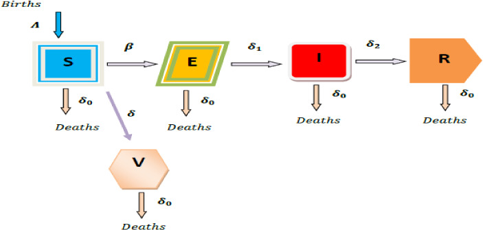
The proposed SEIRV model with vaccination is depicted in Fig. 1 as a flow diagram.

Fig. 1.

The SEIRV model is represented schematically

The SEIRV model [36, 37] with vaccination in the sense of integral order is defined as follows on the basis of the flow diagram:

$$D_{t}S\left(t\right)=\mathrm{\Lambda }-\beta S\left(t\right)I\left(t\right)-{\delta }_{0}S\left(t\right)-\delta S\left(t\right),$$

$$D_{t}E\left(t\right)=\beta S\left(t\right)I\left(t\right)-\left({\delta }_0+{\delta }_1\right)E\left(t\right),$$ 3.2

$$D_{t}I\left(t\right)={\delta }_{1}E\left(t\right)-\left({\delta }_0+{\delta }_2\right)I\left(t\right),$$

$$D_{t}R\left(t\right)={\delta }_{2}I\left(t\right)-{\delta }_{0}R\left(t\right),$$

$$D_{t}V\left(t\right)=\delta S\left(t\right)-{\delta }_{0}V\left(t\right),$$

where

$\mathrm{\Lambda }$: birth rate of susceptible individuals,

$\beta$: the rate of infection of susceptible individuals,

${\delta }_0$: the rate of mortality of all individuals,

$\delta$: the rate of vaccination,

${\delta }_1$: the rate of progression from exposed to infected individuals,

${\delta }_2$: the recovery rate of infected individuals.

In this communication, we consider the SEIRV model using fractional order derivatives with Caputo operator of order $0<\nu <1$.

$${}_{}^C{D}_t^{\nu }S\left(t\right)={\mathrm{\Lambda }}^{\nu }-{\beta }^{\nu }S\left(t\right)I\left(t\right)-{\delta }_0^{\nu }S\left(t\right)-{\delta }^{\nu }S\left(t\right),$$

$${}_{}^C{D}_t^{\nu }E\left(t\right)={\beta }^{\nu }S\left(t\right)I\left(t\right)-\left({\delta }_0^{\nu }+{\delta }_1^{\nu }\right)E\left(t\right),$$ 3.3

$${}_{}^C{D}_t^{\nu }I\left(t\right)={\delta }_1^{\nu }E\left(t\right)-{\delta }_0^{\nu }I\left(t\right)-{\delta }_2^{\nu }I\left(t\right),$$

$${}_{}^C{D}_t^{\nu }R\left(t\right)={\delta }_2^{\nu }I\left(t\right)-{\delta }_0^{\nu }R\left(t\right),$$

$${}_{}^C{D}_t^{\nu }V\left(t\right)={\delta }^{\nu }S\left(t\right)-{\delta }_0^{\nu }V\left(t\right),$$

It is found that the model system’s time dimension (3.3) is correct as both sides of the model system’s equations have dimension ${\left(\mathit{time}\right)}^{-\nu }$ [38]. Next, let us consider $t_0=0$ and disregarded the super script $\nu$ of all parameters and the system becomes:

$${}_{}^C{D}_t^{\nu }S\left(t\right)=\mathrm{\Lambda }-\beta S\left(t\right)I\left(t\right)-{\delta }_{0}S\left(t\right)-\delta S\left(t\right),$$

$${}_{}^C{D}_t^{\nu }E\left(t\right)=\beta S\left(t\right)I\left(t\right)-\left({\delta }_0+{\delta }_1\right)E\left(t\right),$$ 3.4

$${}_{}^C{D}_t^{\nu }I\left(t\right)={\delta }_{1}E\left(t\right)-{\delta }_{0}I\left(t\right)-{\delta }_{2}I\left(t\right),$$

$${}_{}^C{D}_t^{\nu }R\left(t\right)={\delta }_{2}I\left(t\right)-{\delta }_{0}R\left(t\right),$$

$${}_{}^C{D}_t^{\nu }V\left(t\right)=\delta S\left(t\right)-{\delta }_{0}V\left(t\right),$$

The initial conditions are

$$S\left(0\right)=S_0>0,E\left(0\right)=E_0>0,I\left(0\right)=I_0>0,R\left(0\right)=R_0\ge 0,V\left(0\right)=V_0\ge 0$$ 3.5

Positivity and boundedness of Solutions

Proposition

For all $t\ge 0,$ the variables are non-negative.

The closed region $\mathrm{\Omega }=\{\left(S,E,I,R,V\right)\in {\mathbb{R}}^5:0<N\le \frac{\lambda }{{\delta }_0}\}$ is positive invariant for the system (3.4).

Proof

From the model (3.4) we have.

$$\begin{array}{c}{}^C{D}_t^{\nu }\left(S+E+I+R+V\right)\left(t\right)=\lambda -{\delta }_0\left(S+E+I+R\right)\left(t\right).\\ \Rightarrow {}^C{D}_t^{\nu }N\left(t\right)=\lambda -{\delta }_{0}N\left(t\right)\\ \Rightarrow {}^C{D}_t^{\nu }N\left(t\right)+{\delta }_{0}N\left(t\right)=\lambda .\\ \end{array}$$ 3.5

Using Laplace transform, we obtain

$$\begin{array}{c}{p}^{\nu }L\left(N\left(t\right)\right)-p^{\nu -1}N\left(0\right)+{\delta }_{0}L\left(N\left(t\right)\right)=\frac{\lambda }{p}\\ \Rightarrow L\left(N\left(t\right)\right)\left(p^{\nu +1}+{\delta }_0\right)=p^{\nu }N\left(0\right)+\lambda \\ \Rightarrow L\left(N\left(t\right)\right)=\frac{p^{\nu }N\left(0\right)+\lambda }{p^{\nu +1}+{\delta }_0}=\frac{p^{\nu }N\left(0\right)}{p^{\nu +1}+{\delta }_0}+\frac{\lambda }{p^{\nu +1}+{\delta }_0}.\\ \end{array}$$ 3.6

Taking inverse Laplace transform, we have

$$N\left(t\right)=N\left(0\right)E_{\nu ,1}\left(-{\delta }_0{t}^{\nu }\right)+\lambda t^{\nu }{E}_{\nu ,\nu +1}\left(-{\delta }_0{t}^{\nu }\right).$$

According to Mittag–Leffler function,

$$E_{c,d}\left(z\right)=z{E}_{c,c+d}\left(z\right)+\frac{1}{\mathrm{\Gamma }\left(d\right)}.$$

Hence, $N\left(t\right)=\left(N\left(0\right)-\frac{\lambda }{{\delta }_0}\right)E_{\nu ,1}\left(-{\delta }_0{t}^{\nu }\right)+\frac{\lambda }{{\delta }_0}$.

$$\mathrm{Thus}\underset{t\to \infty }{lim}SupN\left(t\right)\le \frac{\lambda }{{\delta }_0}.$$ 3.7

And hence the model (3.4) is bounded above by $\frac{\lambda }{{\delta }_0}$.

Thus $S,E,I,R,$ and $V$ are all positive functions, and the system (3.4) is positive invariant.

Existence and uniqueness of solution

This section demonstrates that the system (3.4) has a unique solution. To begin with, we rewrite system (3.4) in the following manner:

$${}_{}^C{D}_t^{\nu }S\left(t\right)=G_1\left(t,S\left(t\right)\right),$$

$${}_{}^C{D}_t^{\nu }E\left(t\right)=G_2\left(t,E\left(t\right)\right),$$ 3.8

$${}_{}^C{D}_t^{\nu }I\left(t\right)=G_3\left(t,I\left(t\right)\right),$$

$${}_{}^C{D}_t^{\nu }R\left(t\right)=G_4\left(t,R\left(t\right)\right),$$

$${}_{}^C{D}_t^{\nu }V\left(t\right)=G_5\left(t,V\left(t\right)\right),$$

where

$$G_1\left(t,S\left(t\right)\right)=\mathrm{\Lambda }-\beta S\left(t\right)I\left(t\right)-{\delta }_{0}S\left(t\right)-\delta S\left(t\right),G_2\left(t,E\left(t\right)\right)=\beta S\left(t\right)I\left(t\right)-\left({\delta }_0+{\delta }_1\right)E\left(t\right),$$

$$G_3\left(t,I\left(t\right)\right)={\delta }_{1}E\left(t\right)-{\delta }_{0}I\left(t\right)-{\delta }_{2}I\left(t\right),G_4\left(t,R\left(t\right)\right)={\delta }_{2}I\left(t\right)-{\delta }_{0}R\left(t\right),G_5\left(t,V\left(t\right)\right)=\delta S\left(t\right)-{\delta }_{0}V\left(t\right).$$

Taking integral transform on both sides of the Eqs. (3.8), we obtain

$$S\left(t\right)-S\left(0\right)=\frac{1}{\mathrm{\Gamma }\left(\nu \right)}\underset{0}{\overset{t}{\int }}{G}_1\left(p,S\right){(t-p)}^{\nu -1}dp,$$

$$E\left(t\right)-E\left(0\right)=\frac{1}{\mathrm{\Gamma }\left(\nu \right)}\underset{0}{\overset{t}{\int }}{G}_2\left(p,E\right){(t-p)}^{\nu -1}dp,$$

$$I\left(t\right)-I\left(0\right)=\frac{1}{\mathrm{\Gamma }\left(\nu \right)}\underset{0}{\overset{t}{\int }}{G}_3\left(p,I\right){(t-p)}^{\nu -1}dp,$$ 3.9

$$R\left(t\right)-R\left(0\right)=\frac{1}{\mathrm{\Gamma }\left(\nu \right)}\underset{0}{\overset{t}{\int }}{G}_4\left(p,R\right){(t-p)}^{\nu -1}dp,$$

$$V\left(t\right)-V\left(0\right)=\frac{1}{\mathrm{\Gamma }\left(\nu \right)}\underset{0}{\overset{t}{\int }}{G}_5\left(p,V\right){(t-p)}^{\nu -1}dp,$$

The kernels $G_i$, i = 1, 2, 3, 4,5, fulfil the Lipschitz condition and contraction, as demonstrated.

Theorem 1

$G_1$ satisfies the Lipschitz condition and contraction if the following condition holds: $0\le \beta a_1+{\delta }_0+\delta <1.$

Proof

For $S$ and $S_1$,

$$∥G_1\left(t,S\right)-G_1\left(t,S_1\right)∥=∥-\beta I\left(t\right)\left(S\left(t\right)-S_1\left(t\right)\right)-{\delta }_0\left(S\left(t\right)-S_1\left(t\right)\right)-\delta \left(S\left(t\right)-S_1\left(t\right)\right)∥$$

$$\le \left(\beta \Vert I\left(t\right)\Vert +{\delta }_0+\delta \right)\left(\Vert ,S\left(t\right)-S_1\left(t\right),\Vert \right).$$

Suppose $K_1=\beta a_1+{\delta }_0+\delta$, where $I\left(t\right)\le a_1$ is a bounded function.

$$\mathit{So}\Vert G_1\left(t,S\right)-G_1\left(t,S_1\right)\Vert \le K_1\left(\Vert ,S\left(t\right)-S_1\left(t\right)\Vert \right).$$ 3.10

For $G_1$, the Lipschitz condition is obtained, and if $0\le \beta a_1+{\delta }_0+\delta <$ 1, then $G_1$ is a contraction.

In the same manner, $G_j,j=2,3,4,5$ satisfy the Lipschitz condition as follows:

$$∥G_2\left(t,E\right)-G_2\left(t,E_1\right)∥\le K_2\left(∥E\left(t\right)-E_1\left(t\right)∥\right),$$

$$∥G_3\left(t,I\right)-G_3\left(t,I_1\right)∥\le K_3\left(∥I\left(t\right)-I_1\left(t\right)∥\right),$$

$$∥G_4\left(t,R\right)-G_4\left(t,R_1\right)∥\le K_4\left(∥R\left(t\right)-R_1\left(t\right)∥\right),$$

$$∥G_5\left(t,V\right)-G_5\left(t,V_1\right)∥\le K_5\left(∥V\left(t\right)-V_1\left(t\right)∥\right),$$

where $K_2={\delta }_0+{\delta }_1,K_3={\delta }_0+{\delta }_2,K_4={\delta }_0,K_5={\delta }_0.$

For $j=2,3,4,5$, we obtain $0\le K_j<1$, then $G_j$ are contractions. Consider the following recursive patterns, as suggested by system (3.9):

$${\phi }_{1n}\left(t\right)=S_n\left(t\right)-S_{n-1}\left(t\right)=\frac{1}{\mathrm{\Gamma }\left(\nu \right)}\underset{0}{\overset{t}{\int }}\left(G_1\left(p,S_{n-1}\right)-G_1\left(p,S_{n-2}\right)\right){(t-p)}^{\nu -1}dp,$$

$${\phi }_{2n}\left(t\right)=E_n\left(t\right)-E_{n-1}\left(t\right)=\frac{1}{\mathrm{\Gamma }\left(\nu \right)}\underset{0}{\overset{t}{\int }}\left(G_2\left(p,E_{n-1}\right)-G_2\left(p,E_{n-2}\right)\right){(t-p)}^{\nu -1}dp,$$

$${\phi }_{3n}\left(t\right)=I_n\left(t\right)-I_{n-1}\left(t\right)=\frac{1}{\mathrm{\Gamma }\left(\nu \right)}\underset{0}{\overset{t}{\int }}\left(G_3\left(p,I_{n-1}\right)-G_3\left(p,I_{n-2}\right)\right){(t-p)}^{\nu -1}dp,$$

$${\phi }_{4n}\left(t\right)=R_n\left(t\right)-R_{n-1}\left(t\right)=\frac{1}{\mathrm{\Gamma }\left(\nu \right)}\underset{0}{\overset{t}{\int }}\left(G_4\left(p,R_{n-1}\right)-G_4\left(p,R_{n-2}\right)\right){(t-p)}^{\nu -1}dp,$$

$${\phi }_{5n}\left(t\right)=V_n\left(t\right)-V_{n-1}\left(t\right)=\frac{1}{\mathrm{\Gamma }\left(\nu \right)}\underset{0}{\overset{t}{\int }}\left(G_5\left(p,V_{n-1}\right)-G_5\left(p,V_{n-2}\right)\right){(t-p)}^{\nu -1}dp,$$

with $S_0\left(t\right)=S\left(0\right),E_0\left(t\right)=E\left(0\right),I_0\left(t\right)=I\left(0\right),R_0\left(t\right)=R\left(0\right)$ and $V_0\left(t\right)=V\left(0\right)$.

Throughout the above system, we compute the norm of its first equation, and then

$$∥{\phi }_{1n}\left(t\right)∥=∥S_n\left(t\right)-S_{n-1}\left(t\right)∥=∥\frac{1}{\mathrm{\Gamma }\left(\nu \right)}\underset{0}{\overset{t}{\int }}\left(G_1\left(p,S_{n-1}\right)-G_1\left(p,S_{n-2}\right)\right){(t-p)}^{\nu -1}dp∥$$

$\le \frac{1}{\mathrm{\Gamma }\left(\nu \right)}{\sum }_0^t∥\left(G_1\left(p,S_{n-1}\right)-G_1\left(p,S_{n-2}\right)\right){(t-p)}^{\nu -1}∥dp$ .

Possessing Lipschitz’s condition (3.10), we have

$$∥{\phi }_{1n}\left(t\right)∥\le \frac{1}{\mathrm{\Gamma }\left(\nu \right)}{K}_1{\int }_0^t∥{\phi }_{1\left(n-1\right)}\left(p\right)∥dp.$$ 3.11

In similar aspect, we obtain

$$∥{\phi }_{2n}\left(t\right)∥\le \frac{1}{\mathrm{\Gamma }\left(\nu \right)}{K}_2{\int }_0^t∥{\phi }_{2\left(n-1\right)}\left(p\right)∥dp,$$

$$∥{\phi }_{3n}\left(t\right)∥\le \frac{1}{\mathrm{\Gamma }\left(\nu \right)}{K}_3{\int }_0^t∥{\phi }_{3\left(n-1\right)}\left(p\right)∥dp,$$ 3.12

$$∥{\phi }_{4n}\left(t\right)∥\le \frac{1}{\mathrm{\Gamma }\left(\nu \right)}{K}_4{\int }_0^t∥{\phi }_{4\left(n-1\right)}\left(p\right)∥dp,$$

$$∥{\phi }_{5n}\left(t\right)∥\le \frac{1}{\mathrm{\Gamma }\left(\nu \right)}{K}_5{\int }_0^t∥{\phi }_{5\left(n-1\right)}\left(p\right)∥dp.$$

As a result, we may write

$$S_n\left(t\right)=\sum _{i=1}^n{\phi }_{1i}\left(t\right),E_n\left(t\right)=\sum _{i=1}^n{\phi }_{2i}\left(t\right),I_n\left(t\right)=\sum _{i=1}^n{\phi }_{3i}\left(t\right),R_n\left(t\right)=\sum _{i=1}^n{\phi }_{4i}\left(t\right),V_n\left(t\right)=\sum _{i=1}^n{\phi }_{5i}\left(t\right).$$

Theorem 2

A system of solutions described by the SEIRV model (3.4) exists if there exists $t_1$ such that $\left(\frac{1}{\mathrm{\Gamma }\left(\nu \right)}{t}_1{K}_j\right)<1.$

Proof

From (3.11) and (3.12), we have.

$$∥{\phi }_{1n}\left(t\right)∥\le ∥S_n\left(0\right)∥{\left[\frac{1}{\mathrm{\Gamma }\left(\nu \right)}t{K}_1\right]}^n,$$

$$∥{\phi }_{2n}\left(t\right)∥\le ∥E_n\left(0\right)∥{\left[\frac{1}{\mathrm{\Gamma }\left(\nu \right)}t{K}_2\right]}^n,$$

$$∥{\phi }_{3n}\left(t\right)∥\le ∥I_n\left(0\right)∥{\left[\frac{1}{\mathrm{\Gamma }\left(\nu \right)}t{K}_3\right]}^n,$$

$$∥{\phi }_{4n}\left(t\right)∥\le ∥R_n\left(0\right)∥{\left[\frac{1}{\mathrm{\Gamma }\left(\nu \right)}t{K}_4\right]}^n,$$

$$∥{\phi }_{5n}\left(t\right)∥\le ∥V_n\left(0\right)∥{\left[\frac{1}{\mathrm{\Gamma }\left(\nu \right)}t{K}_5\right]}^n.$$

Thus, the system is continuous and has a solution. Now we’ll explain how the functions listed above may be used to construct a model solution (3.9). We make the assumption that

$$S\left(t\right)-S\left(0\right)=S_n\left(t\right)-P_{1n}\left(t\right),$$

$$E\left(t\right)-E\left(0\right)=E_n\left(t\right)-P_{2n}\left(t\right),$$

$$I\left(t\right)-I\left(0\right)=I_n\left(t\right)-P_{3n}\left(t\right),$$

$$R\left(t\right)-R\left(0\right)=R_n\left(t\right)-P_{4n}\left(t\right),$$

$$V\left(t\right)-V\left(0\right)=V_n\left(t\right)-P_{5n}\left(t\right).$$

So

$$\begin{array}{cc}\hfill ∥P_{1n}\left(t\right)∥=& ∥\frac{1}{\mathrm{\Gamma }\left(\nu \right)}\underset{0}{\overset{t}{\int }}\left(G_1\left(p,S\right)-G_1\left(p,S_{n-1}\right)\right)dp∥\hfill \\ \hfill & \le \frac{1}{\mathrm{\Gamma }\left(\nu \right)}\underset{0}{\overset{t}{\int }}∥G_1\left(p,S\right)-G_1\left(p,S_{n-1}\right)∥dp\hfill \\ \hfill & \le \frac{1}{\mathrm{\Gamma }\left(\nu \right)}t{K}_1∥S-S_{n-1}∥.\hfill \\ \hfill \end{array}$$

We get the result by repeating the process.

$$∥P_{1n}\left(t\right)∥\le {\left[\frac{1}{\mathrm{\Gamma }\left(\nu \right)}t\right]}^{n+1}{K}_1^{n+1}k.$$ 3.13

$∥P_{1n}\left(t\right)∥\to 0$ as $n\to \infty$.

Similarly, we may establish that $∥P_{\mathit{jn}}\left(t\right)∥\to 0,j=2,3,4,5$ as $n\to \infty$.

To examine the uniqueness of the solution, we assume that there is another solution of the system, such as $S_1\left(t\right),E_1\left(t\right),I_1\left(t\right),R_1\left(t\right)and{V}_1\left(t\right)$.

Then

$$S\left(t\right)-S_1\left(t\right)=\frac{1}{\mathrm{\Gamma }\left(\nu \right)}\underset{0}{\overset{t}{\int }}\left(G_1\left(p,S\right)-G_1\left(p,S_{n-1}\right)\right)dp.$$

Taking norm we have

$$∥S\left(t\right)-S_1\left(t\right)∥=\frac{1}{\mathrm{\Gamma }\left(\nu \right)}\underset{0}{\overset{t}{\int }}∥G_1\left(p,S\right)-G_1\left(p,S_{n-1}\right)∥dp.$$

From Lipschitz condition (3.10),

$$∥S\left(t\right)-S_1\left(t\right)∥\le \frac{1}{\mathrm{\Gamma }\left(\nu \right)}t{K}_1∥S\left(t\right)-S_1\left(t\right)∥.$$

Thus

$$∥S\left(t\right)-S_1\left(t\right)∥\left(1-\frac{1}{\mathrm{\Gamma }\left(\nu \right)}t{K}_1\right)\le 0.$$ 3.14

Theorem 3

The model system ( 3.4 ) has a unique solution, provided that

$$\left(1-\frac{1}{\mathrm{\Gamma }\left(\nu \right)}t{K}_1\right)>0.$$

Proof

Assuming that condition (3.14) is valid,

$$∥S\left(t\right)-S_1\left(t\right)∥\left(1-\frac{1}{\mathrm{\Gamma }\left(\nu \right)}t{K}_1\right)\le 0.$$

Then $∥S\left(t\right)-S_1\left(t\right)∥=0$. So, we have $S\left(t\right)=S_1\left(t\right)$. Similarly, we can prove that $E\left(t\right)=E_1\left(t\right)$, $I\left(t\right)=I_1\left(t\right)$, $R\left(t\right)=R_1\left(t\right)$, $V\left(t\right)=V_1\left(t\right)$.

Equilibrium Points and Basic Reproduction Number

The disease-free equilibrium points $E_0$ and the epidemic equilibrium point $E_1$ of the system (3.4) are obtained from

$${}^C{D}_t^{\nu }S\left(t\right)={}^C{D}_t^{\nu }E\left(t\right)={}^C{D}_t^{\nu }I\left(t\right)={}^C{D}_t^{\nu }R\left(t\right)={}^C{D}_t^{\nu }V\left(t\right)=0.$$ 3.15

We have $E_0$ = ($\frac{\mathrm{\Lambda }}{{\delta }_0+\delta },0,0,0,\frac{\mathrm{\Lambda }\delta }{{\delta }_0({\delta }_0+\delta )}$) and $E_1=\left(S^{\ast },E^{\ast },I^{\ast },R^{\ast },V^{\ast }\right)$,

where $S^{\ast }$ = $\frac{\left({\delta }_0+{\delta }_1\right)\left({\delta }_0+{\delta }_2\right)}{\beta {\delta }_1}$, $E^{\ast }=\frac{\left({\delta }_0+{\delta }_2\right)}{{\delta }_1}{I}^{\ast }$, $I^{\ast }$ = $\frac{\mathrm{\Lambda }{\delta }_1}{\left({\delta }_0+{\delta }_1\right)\left({\delta }_0+{\delta }_2\right)}-\frac{{\delta }_0+\delta }{\beta }$, $R^{\ast }$ = $\frac{{\delta }_2}{{\delta }_0}{I}^{\ast }$, $V^{\ast }$ = $\frac{\left({\delta }_0+{\delta }_1\right)\left({\delta }_0+{\delta }_2\right)\delta }{\beta {\delta }_0{\delta }_1}$.

The basic reproduction number, indicated by ${\Re }_0$, is the estimated number of secondary cases generated by infection of a single susceptible individual.

Using next generation matrix method [39, 40], the reproduction number (${\Re }_0$) can be obtained from the leading eigen value of the matrix $F{V}^{-1}$ where,

$$F=\left[\begin{array}{cc}0& \frac{\beta \mathrm{\Lambda }}{{\delta }_0+\delta }\\ 0& 0\end{array}\right]\mathit{and}V=\left[\begin{array}{cc}{\delta }_0+{\delta }_1& 0\\ -{\delta }_1& {\delta }_0+{\delta }_2\end{array}\right].$$

$$\mathrm{Therefore},\mathrm{the}\mathrm{reproduction}\mathrm{number}{\Re }_0=\frac{\beta \mathrm{\Lambda }{\delta }_1}{\left({\delta }_0+\delta \right)\left({\delta }_0+{\delta }_1\right)\left({\delta }_0+{\delta }_2\right)}.$$ 3.16

Each parameter is obviously dependent on $\nu .$ So ${\Re }_0$ is a function of $\nu .$ For analysis purpose, we have fixed the value of $\nu$. If we change the value of $\nu$, then all other parametric values will be changed and this will change the value of ${\Re }_0$.

Significance of Sensitivity Parameters

This section shows the impact of altering parameter values on the ${\Re }_0$, reproduction number’s perceived usefulness. The crucial parameter, which might be a critical threshold for illness management, must be identified.

The following are the mathematical representations of ${\Re }_0$’s sensitivity index towards the parameters $\mathrm{\Lambda },\beta$, $\delta ,{\delta }_0,{\delta }_1,{\delta }_2$:

$$\begin{array}{cc}\hfill \frac{\partial {\Re }_0}{\partial \mathrm{\Lambda }}& =\frac{\beta {\delta }_1}{\left({\delta }_0+\delta \right)\left({\delta }_0+{\delta }_1\right)\left({\delta }_0+{\delta }_2\right)},\hfill \\ \hfill \frac{\partial {\Re }_0}{\partial \beta }& =\frac{\mathrm{\Lambda }{\delta }_1}{\left({\delta }_0+\delta \right)\left({\delta }_0+{\delta }_1\right)\left({\delta }_0+{\delta }_2\right)},\frac{\partial {\Re }_0}{\partial \delta }=-\frac{\beta \mathrm{\Lambda }{\delta }_1}{{\left({\delta }_0+\delta \right)}^2\left({\delta }_0+{\delta }_1\right)\left({\delta }_0+{\delta }_2\right)},\hfill \end{array}$$

$$\frac{\partial {\Re }_0}{\partial {\delta }_1}=\frac{\beta \mathrm{\Lambda }{\delta }_0}{\left({\delta }_0+\delta \right){\left({\delta }_0+{\delta }_1\right)}^2\left({\delta }_0+{\delta }_2\right)},\frac{\partial {\Re }_0}{\partial {\delta }_2}=-\frac{\beta \mathrm{\Lambda }{\delta }_1}{{\left({\delta }_0+{\delta }_2\right)}^2\left({\delta }_0+{\delta }_1\right)\left({\delta }_0+\delta \right)},$$

$$\frac{\partial {\Re }_0}{\partial {\delta }_0}=-\frac{\beta \mathrm{\Lambda }{\delta }_1\left[3{\delta }_0^2+2{\delta }_0\left({\delta }_0+\delta +{\delta }_2\right)+\left(\delta {\delta }_1+{\delta }_1{\delta }_2+\delta {\delta }_2\right)\right]}{{\left[\left({\delta }_0+\delta \right)\left({\delta }_0+{\delta }_1\right)\left({\delta }_0+{\delta }_2\right)\right]}^2}.$$

It is inferred that some derivatives seem positive, and that the basic reproductive number ${\Re }_0$ increases as any of the aforementioned positive value parameters $\mathrm{\Lambda },\beta ,{\delta }_1$ is increased. The proportionate reaction to the proportion stimulation is used to calculate the elasticity.

We have

$${\mathrm{E}}_{\mathrm{\Lambda }}=\frac{\mathrm{\Lambda }}{{\Re }_0}\frac{\partial {\Re }_0}{\partial \mathrm{\Lambda }}=1,{\mathrm{E}}_{\beta }=\frac{\beta }{{\Re }_0}\frac{\partial {\Re }_0}{\partial \beta }=1,{\mathrm{E}}_{{\delta }_1}=\frac{{\delta }_1}{{\Re }_0}\frac{\partial {\Re }_0}{\partial {\delta }_1}=\frac{{\delta }_0}{{\delta }_0+{\delta }_1}.$$

As a result, we observed that ${\mathrm{E}}_{\mathrm{\Lambda }},{\mathrm{E}}_{\beta }$ and ${\mathrm{E}}_{{\delta }_1}$ are positive. This means that increasing the values of the parameters $\mathrm{\Lambda },\beta$ and ${\delta }_1$ raises the value of the fundamental reproduction number ${\Re }_0$. The fundamental reproduction number might vary a lot depending on how these factors are changed. A highly sensitive component should be computed with care, since even slight variations might result in significant quantitative systemic changes.

Stability Analysis

For stability analysis, the Jacobianmatrix of the system (3.4) at disease-free equilibrium point $E_0$ is given by $J_0=P,$ where

$$P=\left[\begin{array}{ccc}{P}_{11}& 0& P_{13}\\ 0& P_{22}& P_{23}\\ \begin{array}{c}0\\ \begin{array}{c}0\\ P_{51}\end{array}\end{array}& \begin{array}{c}{P}_{32}\\ \begin{array}{c}0\\ 0\end{array}\end{array}& \begin{array}{c}{P}_{33}\\ \begin{array}{c}{P}_{43}\\ 0\end{array}\end{array}\end{array}\begin{array}{cc}0& 0\\ 0& 0\\ \begin{array}{c}0\\ \begin{array}{c}{P}_{44}\\ 0\end{array}\end{array}& \begin{array}{c}0\\ \begin{array}{c}0\\ P_{55}\end{array}\end{array}\end{array}\right],$$

with $P_{11}=-\left(\delta +{\delta }_0\right)$,$P_{13}=-\beta S_0$,$P_{22}=-\left({\delta }_1+{\delta }_0\right)$,$P_{23}=\beta S_0,P_{32}={\delta }_1$,$P_{33}=-\left({\delta }_0+{\delta }_2\right),P_{44}=-{\delta }_0,P_{55}=-{\delta }_0,P_{43}={\delta }_2$.

Theorem 4

When ${\Re }_0$ When  < 1, the disease-free equilibrium point of the system ( 3.4 ) is locally asymptotically stable, and when ${\Re }_0>1$ , it is unstable.

Proof

The characteristic equation of $J_0$ is given by determinant $\left(P-\lambda I_5\right)=0.$

The roots of the characteristic equation are $-{\delta }_0$, $-{\delta }_0$, $-\left(\delta +{\delta }_0\right)$ and ${\lambda }^2-\lambda \left(P_{22}+P_{33}\right)+\left(P_{22}{P}_{33}-P_{23}{P}_{32}\right)=0$.

By Routh-Hurwitz Criterion, the roots are negative if $\left(P_{22}+P_{33}\right)<0$ and $\left(P_{22}{P}_{33}-P_{23}{P}_{32}\right)>0.$

Now $\left(P_{22}{P}_{33}-P_{23}{P}_{32}\right)>0$

$$=>\left({\delta }_1+{\delta }_0\right)\left({\delta }_0+{\delta }_2\right)-\frac{\beta \mathrm{\Lambda }{\delta }_1}{\left({\delta }_0+\delta \right)}>0$$

$$=>{\Re }_0<1.$$

Since the first three roots are negative and other roots will be negative if ${\Re }_0<1$ and positive if ${\Re }_0>1$.

Therefore the equilibrium point $E_0$ is locally asymptotically stable or unstable according as ${\Re }_0<1$ or ${\Re }_0>1$.

Theorem 5

When ${\Re }_0$ < 1, the disease-free equilibrium point $E_0$ of the system (3.4) is globally asymptotically stable, and unstable when ${\Re }_0>1$.

Proof

Taking the appropriate Lyapunov function into consideration.

$$F=\left({\delta }_1\right)E+\left({\delta }_0+{\delta }_1\right)I.$$

The time fractional derivative of the above function is

$${}_{}^C{D}_t^{\nu }F\left(t\right)=\left({\delta }_1\right){}_{}^C{D}_t^{\nu }E\left(t\right)+\left({\delta }_0+{\delta }_1\right){}_{}^C{D}_t^{\nu }I\left(t\right).$$

From (3.4) we get,

$${}^C{D}_t^{\nu }F\left(t\right)=\left({\delta }_1\right)\left[\beta SI-\left({\delta }_0+{\delta }_1\right)E\right]+\left({\delta }_0+{\delta }_1\right)\left[{\delta }_{1}E-\left({\delta }_0+{\delta }_2\right)I\right]$$

Now,

$$\begin{array}{c}{}_{}^C{D}_t^{\nu }F\left(t\right)=\beta SI{\delta }_1-\left({\delta }_0+{\delta }_1\right)\left({\delta }_0+{\delta }_2\right)I\\ =I\left[\left({\delta }_0+{\delta }_1\right)\left({\delta }_0+{\delta }_2\right)\right]\left[\frac{\beta S{\delta }_1}{\left({\delta }_0+{\delta }_1\right)\left({\delta }_0+{\delta }_2\right)}-1\right]\\ \end{array}$$

Since $S=\frac{\mathrm{\Lambda }}{{\delta }_0+\delta }\le N$, it follows that

$$\begin{array}{c}{}_{}^C{D}_t^{\nu }F\left(t\right)=I\left[\left({\delta }_0+{\delta }_1\right)\left({\delta }_0+{\delta }_2\right)\right]\left[\frac{\beta \mathrm{\Lambda }{\delta }_1}{\left({\delta }_0+\delta \right)\left({\delta }_0+{\delta }_1\right)\left({\delta }_0+{\delta }_2\right)}-1\right]\\ =I\left[\left({\delta }_0+{\delta }_1\right)\left({\delta }_0+{\delta }_2\right)\right]\left[{\Re }_0-1\right]\\ \end{array}$$

Hence if ${\Re }_0<1,$ then ${}_{}^C{D}_t^{\nu }F\left(t\right)<0$. Hence, by LaSalle's extension to Lyapunov’s principle [41, 42], the disease-free equilibrium point $E_0$ is globally asymptotically stable and unstable if ${\Re }_0>1$.

Theorem 6

If ${\Re }_0>1$ , the epidemic equilibrium $E_1=\left(S^{\ast },E^{\ast },I^{\ast },R^{\ast },V^{\ast }\right)$ is locally asymptotically stable.

Proof

The characteristic equation is $\left(-{\delta }_0-\lambda \right)\left(-{\delta }_0-\lambda \right)$(${\lambda }^3+A{\lambda }^2+B\lambda +C)=0$. where

$$A=-\left(G_{11}+G_{22}+G_{33}\right),B=G_{11}\left(G_{22}+G_{33}\right)+\left(G_{22}{G}_{33}-G_{23}{G}_{32}+G_{13}{G}_{21}{G}_{32}\right),$$

$$C=-G_{11}\left(G_{22}{G}_{33}-G_{23}{G}_{32}+G_{13}{G}_{21}{G}_{32}\right),$$

with

$$G_{11}=-\beta I^{\ast }-\delta -{\delta }_0,G_{22}=-{\delta }_0-{\delta }_1,G_{33}=-{\delta }_0-{\delta }_2,G_{23}=\beta S^{\ast },G_{32}={\delta }_1,$$

$$G_{13}=-\beta S^{\ast },G_{23}=\beta I^{\ast },G_{21}=\beta I^{\ast }.$$

Since $A>0,C>0,AB>C$, by Routh-Hurwitz Criterion, the system (3.4) is locally asymptotically stable at $E_1$.

Theorem 7

The epidemic equilibrium $E_1$ is globally asymptotically stable if ${\Re }_0>1$.

Proof

The Goh-Volterra form's non-linear Lyapunov function is defined as.

$$W=\left(S-S^{\ast }-S^{\ast }log\frac{S}{S^{\ast }}\right)+\left(E-E^{\ast }-E^{\ast }log\frac{E}{E^{\ast }}\right)+Q\left(I-I^{\ast }-I^{\ast }log\frac{I}{I^{\ast }}\right).$$

Using Lemma 3 and then the above function’s time fractional derivative is,

$${}_{}^C{D}_t^{\nu }W\left(t\right)\le \left(1-\frac{S^{\ast }}{S}\right){}_{}^C{D}_t^{\nu }S\left(t\right)+\left(1-\frac{E^{\ast }}{E}\right){}_{}^C{D}_t^{\nu }\left(t\right)+Q\left(1-\frac{I^{\ast }}{I}\right){}_{}^C{D}_t^{\nu }I\left(t\right).$$ 4.1

Using system (3.4) we get,

$$\begin{array}{cc}\hfill {}_{}^C{D}_t^{\nu }W\left(t\right)\le & \left(\mathrm{\Lambda }-\beta SI-{\delta }_{0}S-\delta S-\frac{S^{\ast }\left(\mathrm{\Lambda }-\beta SI-{\delta }_{0}S-\delta S\right)}{S}\right)\hfill \\ \hfill & +\left(\left(\beta SI-\left({\delta }_0+{\delta }_1\right)E\right)-\frac{E^{\ast }\left(\beta SI-\left({\delta }_0+{\delta }_1\right)E\right)}{E}\right).\hfill \\ \hfill & +Q\left(\left({\delta }_{1}E-\left({\delta }_0+{\delta }_2\right)I\right)-\frac{I^{\ast }\left({\delta }_{1}E-\left({\delta }_0+{\delta }_2\right)I\right)}{I}\right)\hfill \\ \hfill \end{array}$$ 4.2

We have Eq. (3.4) in steady state,

$$\mathrm{\Lambda }=\beta S^{\ast }{I}^{\ast }+{\delta }_0{S}^{\ast }+\delta S^{\ast }.$$ 4.3

Substituting Eq. (4.3) into (4.2) we have

$$\begin{array}{cc}\hfill {}_{}^C{D}_t^{\nu }W\left(t\right)\le & \left(\beta S^{\ast }{I}^{\ast }+{\delta }_0{S}^{\ast }+\delta S^{\ast }-\beta SI-{\delta }_{0}S-\delta S-\frac{S^{\ast }\left(\beta S^{\ast }{I}^{\ast }+{\delta }_0{S}^{\ast }+\delta S^{\ast }-\beta SI-{\delta }_{0}S-\delta S\right)}{S}\right)\hfill \\ \hfill & +\left(\left(\beta SI-\left({\delta }_0+{\delta }_1\right)E\right)-\frac{E^{\ast }\left(\beta SI-\left({\delta }_0+{\delta }_1\right)E\right)}{E}\right)\hfill \\ \hfill & +Q\left(\left({\delta }_{1}E-\left({\delta }_0+{\delta }_2\right)I\right)-\frac{I^{\ast }\left({\mu }_{1}E-\left({\delta }_0+{\delta }_2\right)I\right)}{I}\right).\hfill \\ \hfill \end{array}$$

Further simplification gives,

$$\begin{array}{cc}\hfill {}_{}^C{D}_t^{\nu }W\left(t\right)\le & \left(\beta S^{\ast }{I}^{\ast }+{\delta }_0{S}^{\ast }+\delta S^{\ast }-{\delta }_{0}S-\delta S-\frac{S^{\ast }\left(\beta S^{\ast }{I}^{\ast }+{\delta }_0{S}^{\ast }+\delta S^{\ast }-\beta SI-{\delta }_{0}S-\delta S\right)}{S}\right)\hfill \\ \hfill & +\left(-\left({\delta }_0+{\delta }_1\right)E)-\frac{E^{\ast }\left(\beta SI-\left({\delta }_0+{\delta }_1\right)E\right)}{E}\right)\hfill \\ \hfill & +Q\left(\left({\delta }_{1}E-\left({\delta }_0+{\delta }_2\right)I\right)-\frac{I^{\ast }\left({\delta }_{1}E-\left({\delta }_0+{\delta }_2\right)I\right)}{I}\right).\hfill \\ \hfill \end{array}$$ 4.4

Adding all infected classes without a single star (*) from (4.4) to zero:

$$S^{\ast }\beta I-\left({\delta }_0+{\delta }_1\right)E+Q\left({\delta }_{1}E-\left({\delta }_0+{\delta }_2\right)I\right)=0.$$ 4.5

The steady state was somewhat perturbed between (3.4) and (4.5), yielding:

$$Q=\frac{S^{\ast }\beta }{\left({\delta }_0+{\delta }_2\right)},\left({\delta }_0+{\delta }_1\right)=\frac{I^{\ast }{S}^{\ast }\beta }{E^{\ast }},{\delta }_1=\frac{\left({\delta }_0+{\delta }_2\right)I^{\ast }}{E^{\ast }}.$$ 4.6

Substituting the expression from (4.6) into (4.4) gives:

$\begin{array}{cc}\hfill {}_{}^C{D}_t^{\nu }W\left(t\right)\le & \left(\beta S^{\ast }{I}^{\ast }+{\delta }_0{S}^{\ast }+\delta S^{\ast }-{\delta }_{0}S-\frac{S^{\ast }\left(\beta S^{\ast }{I}^{\ast }+{\delta }_0{S}^{\ast }-{\delta }_{0}S-\delta S\right)}{S}\right)\hfill \\ \hfill & +\left(-\frac{E^{\ast }\beta SI}{E}+I^{\ast }{S}^{\ast }\beta \right)+\left(-\frac{I^{\ast }{S}^{\ast }E\beta I^{\ast }}{I{E}^{\ast }}+\beta S^{\ast }{I}^{\ast }\right).\hfill \\ \hfill \end{array}$.

We have an arithmetic mean that is greater than the geometric mean.

$$\left(2-\frac{s}{S^{\ast }}-\frac{S^{\ast }}{S}\right)\le 0,\left(3-\frac{S^{\ast }}{S}-\frac{I^{\ast }E}{I{E}^{\ast }}-\frac{S{E}^{\ast }I}{E}\right)\le 0.$$

Hecne,

${}_{}^C{D}_t^{\nu }W\left(t\right)\le 0$ for ${\Re }_0>1$.

Hence $W$ is a Lyapunov function. If ${\Re }_0>1$, the epidemic equilibrium $E_1$ is globally asymptotically stable, according to LaSalle's Invariance Principle [42].

SEIRV Model with Optimal Control

Vaccination is an important tool in the fight against infectious illnesses. The vaccine against Covid-19 has recently been proven to be an effective means of stopping the disease’s transmission. Ding et al. [43] and Agarwal et al. [44] have contributed on optimum control theory in fractional calculus. Pontryagain’s maximal principle [45] strikes at the core of the concept of optimal control in fractional calculus. Our goal is to incorporate the effectiveness of vaccination through a control measure namely $w\left(0\le w\left(t\right)\le 1\right)$ and to identify the best control $w^{\ast }$ to minimize the cost function $J\left(w\right)$ of the control strategy.

$$\mathrm{The}\mathrm{cost}\mathrm{function}J\left(w^{\ast }\right)=min\left(J\left(w\left(t\right)\right)\right)\mathrm{with}J\left(w\right)=\underset{0}{\overset{t_g}{\int }}\left[E+I+A_1{w}^2\right]dt,$$ 5.1

subject to

$${}_{}^C{D}_t^{\nu }S\left(t\right)=\mathrm{\Lambda }-\beta S\left(t\right)I\left(t\right)-{\delta }_{0}S\left(t\right)-wS\left(t\right),S\left(0\right)=S_0>0,$$

$${}_{}^C{D}_t^{\nu }E\left(t\right)=\beta S\left(t\right)I\left(t\right)-\left({\delta }_0+{\delta }_1\right)E\left(t\right),E\left(0\right)=E_0\ge 0,$$ 5.2

$${}_{}^C{D}_t^{\nu }I\left(t\right)={\delta }_{1}E\left(t\right)-{\delta }_{0}I\left(t\right)-{\delta }_{2}I\left(t\right),I\left(0\right)=I_0\ge 0,$$

$${}_{}^C{D}_t^{\nu }R\left(t\right)={\delta }_{2}I\left(t\right)-{\delta }_{0}R\left(t\right),R\left(0\right)=R_0\ge 0,$$

$${}_{}^C{D}_t^{\nu }V\left(t\right)=wS\left(t\right)-{\delta }_{0}V\left(t\right),V\left(0\right)=V_0\ge 0,$$

where $0\le w\left(t\right)\le 1$.

Theorem 8

Let $w\left(t\right)$ be a measurable control function on $\left[0,t_g\right]$, with $w\left(t\right)$ having a value in [0,1]. Then an optimal control $w^{\ast }$ minimizing the objective function $J\left(w\right)$ of (5.1) with.

$$w^{\ast }=max\left\{min\left\{\overline{w},1\right\},0\right\},$$

$$\overline{w}=\overline{w}=\frac{\left({\epsilon }_1-{\epsilon }_5\right)S}{2A_1}$$

where

$\left(S,E,I,R,V\right)$ is the corresponding solution of the system (5.2).

Proof

The Hamiltonian has been analyzed in the following manner:

$$\begin{array}{cc}\hfill \mathbb{H}=& \left[E+I+A_1{w}^2\right]+{\epsilon }_1\left(\mathrm{\Lambda }-\beta S\left(t\right)I\left(t\right)-{\delta }_{0}S\left(t\right)-wS\left(t\right)\right)+{\epsilon }_2\left(\beta S\left(t\right)I\left(t\right)-\left({\delta }_0+{\delta }_1\right)E\left(t\right)\right)\hfill \\ \hfill & +{\epsilon }_3\left({\delta }_{1}E\left(t\right)-{\delta }_{0}I\left(t\right)-{\delta }_{2}I\left(t\right)\right)+{\epsilon }_4\left({\delta }_{2}I\left(t\right)-{\delta }_{0}R\left(t\right)\right)+{\epsilon }_5\left(wS\left(t\right)-{\delta }_{0}V\left(t\right)\right),\hfill \\ \hfill \end{array}$$ 5.3

with

${\epsilon }_i\left(t\right)$, i = 1, 2, 3, 4, 5 are the adjoint variables with ${\epsilon }_i\left(t_g\right)=0,$ expressed in terms canonical equations:

$${}^{\mathit{RL}}{D}_t^{\nu }{\epsilon }_1\left(t\right)=-\frac{\partial \mathbb{H}}{\partial S}={\epsilon }_1\left(\beta I\left(t\right)+{\delta }_0-w\right)-{\epsilon }_2\left(\beta I\left(t\right)\right)-{\epsilon }_5\left(w\right),$$

$${}^{\mathit{RL}}{D}_t^{\nu }{\epsilon }_2\left(t\right)=-\frac{\partial \mathbb{H}}{\partial E}=-1+{\epsilon }_2\left(\left({\delta }_0+{\delta }_1\right)E\left(t\right)\right)-{\epsilon }_3\left({\delta }_1\right),$$ 5.4

$${}^{\mathit{RL}}{D}_t^{\nu }{\epsilon }_3\left(t\right)=-\frac{\partial \mathbb{H}}{\partial I}=-1+{\epsilon }_1\left(\beta S\left(t\right)\right)-{\epsilon }_2\left(\beta S\left(t\right)\right)+{\epsilon }_3\left({\delta }_0+{\delta }_2\right)-{\epsilon }_4\left({\delta }_2\right),$$

$${}^{\mathit{RL}}{D}_t^{\nu }{\epsilon }_4\left(t\right)=-\frac{\partial \mathbb{H}}{\partial R}={\epsilon }_4\left({\delta }_0\right),$$

$${}^{\mathit{RL}}{D}_t^{\nu }{\epsilon }_5\left(t\right)=-\frac{\partial \mathbb{H}}{\partial V}={\epsilon }_5\left({\delta }_0\right).$$

As a result, the issue of determining $w^{\ast }$ that minimizes $\mathcal{H}$ in the presence of (5.2) is recast as minimizing the Hamiltonian with regard to the control. We then establish the following optimum condition using the Pontryagin principle:

$$\frac{\partial \mathbb{H}}{\partial w}=2A_{1}w-\left({\epsilon }_1-{\epsilon }_5\right)S=0,$$ 5.5

which may be solved using state and adjoint variables to yield

$$\overline{w}=\frac{\left({\epsilon }_1-{\epsilon }_5\right)S}{2A_1}.$$ 5.6

For the best control $w^{\ast }$, take into account the control constraints as well as the sign of $\frac{\partial \mathbb{H}}{\partial w}$.

As a result, we have

$$w^{\ast }=\left\{\begin{array}{c}0if\frac{\partial \mathbb{H}}{\partial w}<0\\ \\ \overline{w}if\frac{\partial \mathbb{H}}{\partial w}=0\\ \\ 1if\frac{\partial \mathbb{H}}{\partial w}>0\end{array}\right)$$ 5.7

and $w^{\ast }=max\left\{min\left\{\overline{w},1\right\},0\right\}$ where $\overline{w}=\frac{\left({\epsilon }_1-{\epsilon }_5\right)S}{2A_1}$.

By substituting $w^{\ast }$ to the equation, the optimal condition may be determined for the system (5.2).

Adam-Bashforth-Moulton Predictor–Corrector Scheme for the SEIRV Model

The Adams–Bashforth-Moulton strategy is the most widely used numerical technique for addressing any fractional order initial value problems.

Let’s look at the fractional differential equation below.

$${}^C{D}_t^{\nu }{F}_j\left(t\right)=g_j\left(t,F_j\left(t\right)\right),F_j^r\left(0\right)=F_{j0}^r,$$ 6.1

$$r=0,1,2,\dots ,\nu ,j\in \mathbb{N}$$

where $F_{j0}^r$ is the arbitrary real number, $\nu >0$ and the fractional differential operator $D_t^{\nu }$ is identical to the well-known Volterra integral equation in the Caputo sense.

$$F_j\left(t\right)={\sum }_{n=0}^{\nu -1}{F}_{j0}^r\frac{t^n}{n!}+\frac{1}{\mathrm{\Gamma }\left(\mathrm{\nu }\right)}{\int }_0^t{(t-u)}^{\nu -1}{g}_j\left(u,F_j\left(u\right)\right)du,j\in \mathbb{N}.$$ 6.2

Using Adam’s-Bashforth-Moulton predictor–corrector scheme, we explore the numerical solution of a fractional order SEIRV model with vaccination. The algorithm is described in the following manner.

Let $h=\frac{T}{\widehat{m}},t_n=nh,n=0,1,2,\dots ,\widehat{m}.$

Corrector formulae:

$$S_{n+1}=S_0+\frac{h^{\nu }}{\mathrm{\Gamma }\left(\nu +2\right)}\left(\mathrm{\Lambda }-\beta S_{n+1}^p{I}_{n+1}^p-{\delta }_0{S}_{n+1}^p-\delta S_{n+1}^p\right)+\frac{h^{\nu }}{\mathrm{\Gamma }\left(\nu +2\right)}{\sum }_{j=0}^n{\alpha }_{j,n+1}\left(\mathrm{\Lambda }-\beta S_j{I}_j-{\delta }_0{S}_j-\delta S_j\right),$$

$$E_{n+1}=E_0+\frac{h^{\nu }}{\mathrm{\Gamma }\left(\nu +2\right)}\left(\beta S_{n+1}^p{I}_{n+1}^p-\left({\delta }_0+{\delta }_1\right)E_{n+1}^p\right)+\frac{h^{\nu }}{\mathrm{\Gamma }\left(\nu +2\right)}{\sum }_{j=0}^n{\alpha }_{j,n+1}\left(\beta S_j{I}_j-\left({\delta }_0+{\delta }_1\right)E_j\right),$$

$$I_{n+1}=I_0+\frac{h^{\nu }}{\mathrm{\Gamma }\left(\nu +2\right)}\left({\delta }_1{E}_{n+1}^p-\left({\delta }_0+{\delta }_2\right)I_{n+1}^p\right)+\frac{h^{\nu }}{\mathrm{\Gamma }\left(\nu +2\right)}{\sum }_{j=0}^n{\alpha }_{j,n+1}\left({\delta }_1{E}_j-\left({\delta }_0+{\delta }_2\right)I_j\right),$$

$$R_{n+1}=R_0+\frac{h^{\nu }}{\mathrm{\Gamma }\left(\nu +2\right)}\left({\delta }_2{I}_{n+1}^p-{\delta }_0{R}_{n+1}^p\right)+\frac{h^{\nu }}{\mathrm{\Gamma }\left(\nu +2\right)}{\sum }_{j=0}^n{\alpha }_{j,n+1}\left({\delta }_2{I}_j-{\delta }_0{R}_j\right),$$

$$V_{n+1}=V_0+\frac{h^{\nu }}{\mathrm{\Gamma }\left(\nu +2\right)}\left(\delta S_{n+1}^p-{\delta }_0{V}_{n+1}^p\right)+\frac{h^{\nu }}{\mathrm{\Gamma }\left(\nu +2\right)}{\sum }_{j=0}^n{\alpha }_{j,n+1}\left(\delta S_j-{\delta }_0{V}_j\right).$$ 6.3

Predictor formulae:

$$S_{n+1}^p=S_0+\frac{1}{\mathrm{\Gamma }\left(\nu \right)}{\sum }_{j=0}^n{\mathrm{\Theta }}_{j,n+1}\left(\mathrm{\Lambda }-\beta S_j{I}_j-{\delta }_0{S}_j-\delta S_j\right),$$

$$E_{n+1}^p=E_0+\frac{1}{\mathrm{\Gamma }\left(\nu \right)}{\sum }_{j=0}^n{\mathrm{\Theta }}_{j,n+1}\left(\beta S_j{I}_j-\left({\delta }_0+{\delta }_1\right)E_j\right),$$ 6.4

$$I_{n+1}^p=I_0+\frac{1}{\mathrm{\Gamma }\left(\nu \right)}{\sum }_{j=0}^n{\mathrm{\Theta }}_{j,n+1}\left({\delta }_1{E}_j-\left({\delta }_0+{\delta }_2\right)I_j\right),$$

$$R_{n+1}^p=R_0+\frac{1}{\mathrm{\Gamma }\left(\nu \right)}{\sum }_{j=0}^n{\mathrm{\Theta }}_{j,n+1}\left({\delta }_2{I}_j-{\delta }_0{R}_j\right),$$

$$V_{n+1}^p=V_0+\frac{1}{\mathrm{\Gamma }\left(\nu \right)}{\sum }_{j=0}^n{\mathrm{\Theta }}_{j,n+1}\left(\delta S_j-{\delta }_0{V}_j\right),$$

where

$${\nu }_{j,n+1}=\left\{\begin{array}{c}{n}^{\nu +1}-\left(n-\nu \right){(n+1)}^{\nu },\hfill \\ {\left(n-j+2\right)}^{\nu +1}+{(n-j)}^{\nu +1}-2{(n-j+1)}^{\nu +1},\hfill \\ 1,\hfill \end{array}\right)\begin{array}{c}ifj=0,\hfill \\ if0\le j\le n,\hfill \\ ifj=1,\hfill \end{array}.$$

and

$${\mathrm{\Theta }}_{j,n+1}=\frac{h^{\nu }}{\nu }\left[{\left(n+1-j\right)}^{\nu }-\left({n-j)}^{\nu }\right)\right],0\le j\le n.$$

Numerical Simulation and Discussion

In this section, we perform rigorous numerical simulations to evaluate and verify the analytical results of our model system (3.4). Using mathematical software MATLAB (2018a version), we have employed Adam’s-Bashforth-Moulton predictor–corrector scheme to obtain numerical solution to the system (3.4).

We investigate numerical simulations of the model system (3.4) for India in the Caputo sense, using the parameters listed in Table 1. We estimate and anticipate the progression of the COVID-19 pandemic using recent Indian data up to the 10th of August 2021 [4]. In the India scenario, Table 1 is utilized for simulation. The following figures were produced to examine the behavior of the model (3.4) under various initial conditions.

Table 1.

Estimated values of parameters for India:

Parameter	Value	References
$\mathrm{\Lambda }$	0.0182	[46]
$\beta$	0.476	[47]
${\delta }_1$	0.071	[48]
${\delta }_2$	0.286	[47]
${\delta }_0$	0.0073	[46]
$\delta$	0.01	Model to fit

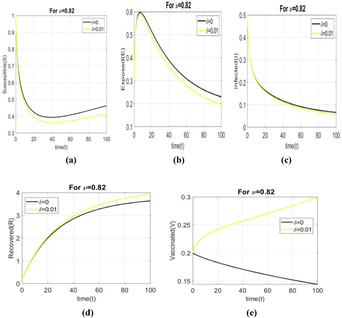
Figure 2 demonstrates the dynamical behavior of all individuals for fractional order $\nu =0.82.$ The comparison of the number of susceptible, infected, exposed and recovered individuals in case of $\delta =0$ and $\delta =0.01$ is quite obvious.The number of susceptible individualsis more for $\delta =0$ than $\delta =0.01.$ Similar is the case with exposed individuals and infected individuals. However, in case of recoveredindividuals, it is just the opposite, due to obvious reasons. Now, the recovered individuals will be more in case of $\delta =0.01$ than in case of $\delta =0$.

Fig. 2.

Comparison of dynamical behaviour of all individuals with respect to time for fractional order $\nu =0.82$, $\delta =0$ and $\delta =0.01$

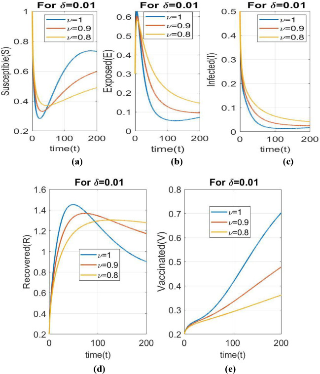
Figure 3 depicts the dynamical behavior of all individuals with a vaccination rate of 0.01 at fractional orders of $\nu =0.8,0.9,1$ and the value of ${\Re }_0$ is $1.55$. The purpose of this study is to demonstrate the importance of the COVID-19 vaccination rate. When we enforced a vaccination rate, the basic reproduction number decreases.

Fig. 3.

Dynamical behaviour of all individuals with respect to time with a vaccination rate, $\delta =0.01$ and fractional order $\nu =0.8,0.9,1$

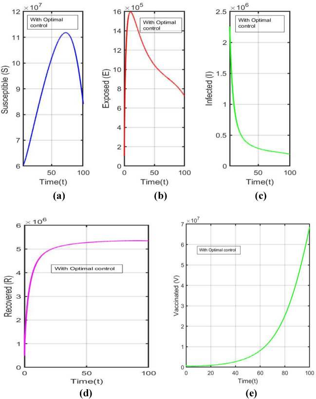
Figure 4a-e shows the time series of susceptible individuals, exposed individuals, infected individuals, recovered individuals and vaccinated individuals across a time period of [0,100] with optimal control taking fractional order ν = 1.

Fig. 4.

With respect to time, the time series of the model system (3.3) corresponds to Table 1

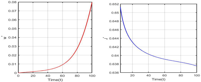
Vaccination is a critical component in preventing people from COVID-19, and various ideas have been proposed in which vaccination rates are viewed as quite beneficial. As a result, the addition of the vaccination parameter decreases the reproduction number ${\Re }_0$. For the simulation of the optimal control problem subject to the model (3.3) corresponding to Table 1 in the India scenario, we used a final time of $t_g=100$. Figure 5 depicts the time series of optimal control variable $w^{\ast }$ and optimal cost $J^{\ast }$.

Fig. 5.

Time series of optimal control variable $w^{\ast }$ and optimal cost $J^{\ast }$ with parameter values corresponding to Table 1

Data Fitting and Model Validation

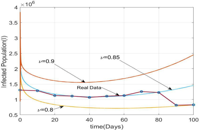
The data fitting and model validation of the system (3.4) for Infected population in Brazil are described in this section. From the 10th of April to the 19th of July, 2021, we compared the model values with the real scenario for Brazil. The total initial population of Brazil is around $209500000$ [4]. The parametric values are given in Table 2. We have taken $t=1$ day as time unit and $t=100$ as final time. Table 3 recommends day wise Infected population from 10th April, 2021 to 19th July, 2021. Figure 6 depict time series solution of Infected population of the system (3.4) for Table 2 taking $\nu =0.8,0.85,0.9.$

Table 2.

The estimated parametric values are as follows in Brazil

Parameter	Value	References
$\mathrm{\Lambda }$	0.0187	[46]
$\beta$	0.32	[47]
${\delta }_1$	0.344	[48]
${\delta }_2$	0.041	[47]
${\delta }_0$	0.0063	[46]
$\delta$	0.01	Model to fit

Table 3.

Day wise Infected population of Brazil from 10th April, 2021 to 19th July, 2021

Day	Infected population
10/04/2021	1,269,000
20/04/2021	1,285,000
30/04/2021	1,270,000
10/05/2021	1,111,000
20/05/2021	1,068,000
30/05/2021	1,108,000
09/06/2021	1,128,000
19/06/2021	1,257,000
29/06/2021	1,227,000
09/07/2021	813,700
19/07/2021	825,000

Fig. 6.

Time series solution of Infected population of the system (3.4) for Table 2 taking $\nu =0.8,0.85,0.9.$

Conclusion

In this paper we have discussed the optimal control of fractional order SEIRV model with vaccination as the control parameter $w$. Based on the COVID-19 cases data in India, collected upto 10th August, 2021, we estimated the basic reproduction number ${\Re }_{0}withoutvaccination$ to be 3.67 and with vaccination to be 1.55. The fractional-order derivatives are usually more suitable in modeling since the choice of the derivative order provides one more degree of freedom and this leads to better fit to the real time data with less error than the integer-order model. A comparison of the number of individuals in different compartments for $\nu =0.82$ has been presented in Fig. 2 in case of $\delta =0$ and $\delta =0.01$. The stability analysis of the model shows that the system is locally as well as globally asymptotically stable at disease-free equilibrium point $E_0$ when ${\Re }_0$ < 1 and at epidemic equilibrium $E_1$ when ${\Re }_0$ > 1. Sensitivity analysis shows that ${\Re }_0$ is directly proportional to thebirth rate of susceptible individuals $\mathrm{\Lambda },$ the rate of infection of susceptible individuals $\beta$ and the rate of progression from exposed to infected individuals ${\delta }_1$, all of which may be controlled with the effective execution of vaccination drives. We have used the Pontryagin’s Maximum Principle to provide the necessary conditions needed for the existence of the optimal solution to the optimal control problem. Adam-Bashforth-Moulton predictor–corrector technique has been used to obtain numerical solutions to the system. Numerical simulations are presented using MATLAB to validate the efficacy and impact of the control parameter. It is evident that if the control measure $w$ is employed then the transmission of the disease may be checked and eradicated. Additionally, the optimal control value $w^{\ast }$ has been determined in Theorem 8 to minimize the cost of vaccination given by $J\left(w\right)={\int }_0^{t_g}\left[E+I+A_1{w}^2\right]dt$. We have assumed a final time $t_g=100$ for optimal control. The order of derivative can differ from region to region. If we vary the order of derivatives while keeping other parametric values fixed, the results will be different (Fig. 6). This demonstrates that the order of derivative is important in system simulation. We have comparatively studied the model values and real scenario of Brazil starts from 10th April 2021 and continues up to 100 days. It has been observed that our model fits with $\nu =0.85$ with realistic data.

Author Contributions

Animesh Mahata: Data curation, Software, Investigation. Subrata Paul: Conceptualization, Methodology. Supriya Mukherjee: Methodology, Validation. Meghadri Das: Software, Validation. Banamali Roy: Supervision, Writing—review & editing.

Funding

None.

Data Availability

There is nothing left after reporting all of the data needed for numerical simulations and comparisons in the tables and depicting it in the graphical representations.

Declarations

Conflict of interest

There are no conflicts of interest declared by the authors.

Ethical approval

All of the authors participated directly and actively involved in the considerable effort that led to the publication of the article, and they will be held accountable for its content. This manuscript is the authors’ original work, and it has never been published earlier. The manuscript is not being considered for publication anywhere at this time. The work accurately and completely represents the authors’ own research and analysis.

Consent for publication

The authors state that they have no known conflicting financial interests or personal connections that might have influenced the research presented in this publication.

References

- 1.Tyrrell, D.A., Bynoe, M.L.: Cultivation of viruses from a high proportion of patients with colds. Lancet (1966) [DOI] [PubMed]
- 2.Wang C, Horby PW, Hayden FG, Gao GF. A novel coronavirus outbreak of global health concern. The Lancet. 2020;395(10223):470–473. doi: 10.1016/S0140-6736(20)30185-9. [DOI] [PMC free article] [PubMed] [Google Scholar]
- 3.Centers for disease control and prevention: 2019 novel coronavirus. https://www.cdc.gov/coronavirus/2019-ncov (2020)
- 4.https://www.worldometers.info/coronavirus/
- 5.Dietz K, Heesterbeek JA. Bernoulli was ahead of modern epidemiology. Nature. 2000;408(6812):513–514. doi: 10.1038/35046270. [DOI] [PubMed] [Google Scholar]
- 6.Kermack NO, Mackendrick AG. Contribution to mathematical theory of epidemics. P. Roy. Soc. Lond. A. Mat. US. 1927;115(772):700–721. doi: 10.1098/rspa.1927.0118. [DOI] [Google Scholar]
- 7.Blackwood JC, Childs LM. An introduction to compartmental modeling for the budding infectious disease modeler. Lett. Biomath. 2018;5(1):195–221. doi: 10.30707/LiB5.1Blackwood. [DOI] [Google Scholar]
- 8.Biazar J. Solution of the epidemic model by Adomian decomposition method. Appl. Math. Comput. 2006;173:1101–1106. [Google Scholar]
- 9.Shereen MA, Khan S. COVID-19 infection: origin, transmission, and characteristics of human coronaviruses. J. Adv. Res. 2020;24:91–98. doi: 10.1016/j.jare.2020.03.005. [DOI] [PMC free article] [PubMed] [Google Scholar]
- 10.Das P, Upadhyay RK, Misra AK, Rihan FA, Das P, Ghosh D. Mathematical model of COVID-19 with comorbitity and controlling using non-pharmaceutical interventions and vaccination. Nonlin. Dyn. 2021 doi: 10.1007/s11071-021-06517-w. [DOI] [PMC free article] [PubMed] [Google Scholar]
- 11.Das P, Nadim SS, Das S, Das P. Dynamics of COVID-19 transmission with comorbidity:a data driven modelling based approach. Nonlin. Dyn. 2021 doi: 10.1007/s11071-021-06324-3. [DOI] [PMC free article] [PubMed] [Google Scholar]
- 12.Ghanbari B, Kumar S, Kumar R. A study of behaviour for immune and tumor cells in immune genetic tumour model with non-singular fractional derivative. Chaos Solitons Fractals. 2020;133:109619. doi: 10.1016/j.chaos.2020.109619. [DOI] [Google Scholar]
- 13.Ullah S, Khan MA, Farooq M, Hammouch Z, Baleanu D. A fractional model for the dynamics of tuberculosis infection using Caputo-Fabrizio derivative. Discrete Contin. Dyn. Syst. Ser. S. 2020;13(3):975–993. doi: 10.3934/dcdss.202005. [DOI] [Google Scholar]
- 14.Shaikh AS, Nisar KS. Transmission dynamics of fractional order typhoid fever model using Caputo-Fabrizio operator. Chaos Solitons Fractals. 2019;128:355–365. doi: 10.1016/j.chaos.2019.08.012. [DOI] [Google Scholar]
- 15.Erturk VS, Zaman G, Momani S. A numeric analytic method for approximating a giving up smoking model containing fractional derivatives. Comput. Math. Appl. 2012;64:3068–3074. doi: 10.1016/j.camwa.2012.02.002. [DOI] [Google Scholar]
- 16.Bushnaq S, Khan S, Shah K, Zaman G. Mathematical analysis of HIV/AIDS infection model with Caputo-Fabrizio fractional derivative. Cogent Math. Stat. 2018;5:1432521. doi: 10.1080/23311835.2018.1432521. [DOI] [Google Scholar]
- 17.Tang B, Wang X, Li Q, Bragazzi NL, Tang S, Xiao Y, Wu J. Estimation of the transmission risk of the 2019-nCoV and its implication for public health interventions. J. Clin. Med. 2020;9(2):462. doi: 10.3390/jcm9020462. [DOI] [PMC free article] [PubMed] [Google Scholar]
- 18.Sontakke BR, Shaikh AS, Nisar KS. Approximate solutions of a generalized Hirota-Satsuma coupled KdV and a coupled mKdV systems with time fractional derivatives. Malaysian J. Math. Sci. 2018;12(2):173–193. [Google Scholar]
- 19.Kumar S, Kumar A, Baleanu D. Two analytical methods for time-fractional nonlinear coupled Boussinesq–Burger’s equations arise in propagation of shallow water waves. Nonlinear Dyn. 2016;85:699–715. doi: 10.1007/s11071-016-2716-2. [DOI] [Google Scholar]
- 20.Shaikh A, Sontakke BR. Impulsive initial value problems for a class of implicit fractional differential equations. Comput. Methods Differ. Equ. 2020;8(1):141–154. [Google Scholar]
- 21.Daftardar-Gejji V, Jafari H. An iterative method for solving nonlinear functional equations. J. Math. Anal. Appl. 2006;316:753–763. doi: 10.1016/j.jmaa.2005.05.009. [DOI] [Google Scholar]
- 22.Garrappa R. On linear stability of predictor–corrector algorithms for fractional differential equations. Int. J. Comput. Math. 2010;87(10):2281–2290. doi: 10.1080/00207160802624331. [DOI] [Google Scholar]
- 23.Das M, Samanta GP. A prey-predator fractional order model with fear effect and group defense. Int. J. Dyn. Control. 2020 doi: 10.1007/s40435-020-00626-x. [DOI] [Google Scholar]
- 24.Baleanu D, Sajjadi SS, Jajarmi A, Defterli O, Asad JH. The fractional dynamics of a linear triatomic molecule. Rom. Rep. Phys. 2021;73(1):105. [Google Scholar]
- 25.Ucar S. Analysis of a basic SEIRA model with Atangana-Baleanu derivative. AIMS Math. 2020;5(2):1411–1424. doi: 10.3934/math.2020097. [DOI] [Google Scholar]
- 26.Baleanu D, Sajjadi SS, Jajarmi A, Defterli O. On a nonlinear dynamical system with both chaotic and non-chaotic behaviours: a new fractional analysis and control. Adv. Differ. Equ. 2021;2021:234. doi: 10.1186/s13662-021-03393-x. [DOI] [Google Scholar]
- 27.Baleanu D, Zibaei S, Namjoo M, Jajarmi A. A nonstandard finite difference scheme for the modelling and nonidentical synchronization of a novel fractional chaotic system. Adv. Diff. Equ. 2021;2021:308. doi: 10.1186/s13662-021-03454-1. [DOI] [Google Scholar]
- 28.Baleanu D, Sajjadi SS, Asad JH, Jajarmi A, Estiri E. Hyperchaotic behaviours, optimal control, and synchronization of a nonautonomous cardiac conduction system. Adv. Differ. Equ. 2021;2021:157. doi: 10.1186/s13662-021-03320-0. [DOI] [Google Scholar]
- 29.Kilbas, A., Srivastava, H., Trujillo, J.: Theory and Applications of Fractional Differential Equations, Vol. 204, North-Holland Mathematics Studies, (2006)
- 30.Losada J, Nieto JJ. Properties of the new fractional derivative without singular kernel. Prog. Fract. Differ. Appl. 2015;1(2):87–92. [Google Scholar]
- 31.Caputo M, Fabrizio M. A new definition of fractional derivative without singular kernel. Prog. Fract. Differ. Appl. 2015;1(2):73–85. [Google Scholar]
- 32.Kexue L, Jigen P. Laplace transform and fractional differential equations. Appl. Math. Lett. 2011;24:2019–2023. doi: 10.1016/j.aml.2011.05.035. [DOI] [Google Scholar]
- 33.Petras I. Fractional-Order Nonlinear Systems: Modeling Aanlysis and Simulation. Beijing, China: Higher Education Press; 2011. [Google Scholar]
- 34.Liang S, Wu R, Chen L. Laplace transform of fractional order differential equations. Electron. J. Differ. Equ. 2015;2015(139):1–15. [Google Scholar]
- 35.Li Y, Chen Y, Podlubny I. Stability of fractional-order nonlinear dynamic systems: Lyapunov direct method and generalized Mittag-Leffler stability. Comput. Math. Appl. 2010;59:1810–1821. doi: 10.1016/j.camwa.2009.08.019. [DOI] [Google Scholar]
- 36.Zhang Z, Kundu S, Tripathi JP, Bugalia S. Stability and Hopf bifurcation analysis of an SVEIR epidemic model with vaccination and multiple time delay. Chaos Solitons Fractals. 2019;131:109483. doi: 10.1016/j.chaos.2019.109483. [DOI] [Google Scholar]
- 37.Upadhyay RK, Kumari S, Misra AK. Modeling the virus dynamics in computer network with SVEIR model and nonlinear incident rate. J. Appl. Math. Comput. 2017;54:485–509. doi: 10.1007/s12190-016-1020-0. [DOI] [Google Scholar]
- 38.Dokoumetzidis A, Magin R, Macheras P. A commentary on fractionalization ofmulti-compartmental models. J. Pharmacokinet Pharmacodyn. 2010;37:203–207. doi: 10.1007/s10928-010-9153-5. [DOI] [PubMed] [Google Scholar]
- 39.Zhu LH, Wang XW, Zhang HH, Shen SL, Li YM, Zhou YD. Dynamics analysis and optimal control strategy for a SIRS epidemic model with two discrete time delays. Phys. Scr. 2020;95:035213. doi: 10.1088/1402-4896/ab495b. [DOI] [Google Scholar]
- 40.Pongkitivanichkul C, Samart D, Tangphati T, Koomhin P, Pimton P, Dam-o P, Payaka A, Channuie P. Estimating the size of COVID-19 epidemic outbreak. Phys. Scr. 2020;95:085206. doi: 10.1088/1402-4896/ab9bdf. [DOI] [Google Scholar]
- 41.Li MY, Smith HL, Wang L. Global dynamics of an SEIR epidemic model with vertical transmission. SIAM J Appl. Math. 2001;62:58. doi: 10.1137/S0036139999359860. [DOI] [Google Scholar]
- 42.Perko L. Differential Equations and Dynamical Systems. New York: Springer; 2000. [Google Scholar]
- 43.Ding Y, Wang Z, Ye H. Optimal control of a fractional-order hiv immune system with memory. IEEE Trans. Control Syst. Technol. 2012;20(3):763–769. doi: 10.1109/TCST.2011.2153203. [DOI] [Google Scholar]
- 44.Agarwal OP. A general formulation and solution scheme for fractional optimal control problems. Nonlinear Dyn. 2004;38(1–4):323–337. doi: 10.1007/s11071-004-3764-6. [DOI] [Google Scholar]
- 45.Kamocki R. Pontryagin maximum principle for fractional ordinary optimal control problems. Math. Methods Appl. Sci. 2014;37(11):1668–1686. doi: 10.1002/mma.2928. [DOI] [Google Scholar]
- 46.https://data.worldbank.org/indicator/SP.DYN.CBRT.IN?locations=IN
- 47.Paul S, Mahata A, Ghosh U, Roy B. SEIR epidemic model and scenario analysis of COVID-19 pandemic. Ecolo. Gene. Genom. 2021;19:100087. doi: 10.1016/j.egg.2021.100087. [DOI] [PMC free article] [PubMed] [Google Scholar]
- 48.Gaff H, Schaefer E. Optimal control applied to vaccination and treatment strategies for various epidemiological models. Math. Biosci. Eng. 2009;6:469–492. doi: 10.3934/mbe.2009.6.469. [DOI] [PubMed] [Google Scholar]
Associated Data
This section collects any data citations, data availability statements, or supplementary materials included in this article.
Data Availability Statement