Modeling the dynamics of COVID-19 pandemic with implementation of intervention strategies

Abstract

The ongoing COVID-19 epidemic spread rapidly throughout India, with 34,587,822 confirmed cases and 468,980 deaths as of November 30, 2021. Major behavioral, clinical, and state interventions have implemented to mitigate the outbreak and prevent the persistence of the COVID-19 in human-to-human transmission in India and worldwide. Hence, the mathematical study of the disease transmission becomes essential to illuminate the real nature of the transmission behavior and control of the diseases. We proposed a compartmental model that stratify into nine stages of infection. The incidence data of the SRAS-CoV-2 outbreak in India was analyzed for the best fit to the epidemic curve and we estimated the parameters from the best fitted curve. Based on the estimated model parameters, we performed a short-term prediction of our model. We performed sensitivity analysis with respect to $R_0$ and obtained that the disease transmission rate has an impact in reducing the spread of diseases. Furthermore, considering the non-pharmaceutical and pharmaceutical intervention policies as control functions, an optimal control problem is implemented to reduce the disease fatality. To mitigate the infected individuals and to minimize the cost of the controls, an objective functional has been formulated and solved with the aid of Pontryagin’s maximum principle. This study suggest that the implementation of optimal control strategy at the start of a pandemic tends to decrease the intensity of epidemic peaks, spreading the maximal impact of an epidemic over an extended time period. Our numerical simulations exhibit that the combination of two controls is more effective when compared with the combination of single control as well as no control.

Introduction

The novel coronavirus is bizarre due to several causes, making its transmission unpredictable and hard to control due to its peculiar epidemiological traits. In December 2019, the COVID-19 pandemic has started in Wuhan city of Hubei Province, the Republic of China, caused by the severe acute respiratory syndrome coronavirus-2 (SARS-CoV-2) and China became the epicenter, and has now spread throughout the world [1]. As of November 30, 2021, the total number of confirmed cases 26,14,35,768 total number of deaths 52,07,634 [2]. The worldwide pandemic resulting from SARS-CoV-2 was preceded by other two epidemics of human coronavirus, namely Middle East respiratory syndrome coronavirus (MERS-CoV) and severe acute respiratory syndrome coronavirus (SARS-CoV) infections [3], posing the tremendous menace to the economy and global public health after the 2nd World War [4]. Presently one of the major problems is that there is no clear picture or consensus on the future progression of the COVID-19 pandemic. The possibilities of the source of the COVID-19 transmission incorporate (but not limited to) animals, human to human and intermediate animal vectors [3].

Due to non-appearance of any pharmaceutical interventions, government of different countries is incorporating different policy to control this pandemic and the most common one is the implementation of lockdown to maintain the social distancing, and contact tracing [5]. This is an excellent measure to control the spreading of the COVID-19, but from an economic view point, the nationwide lockdown may be the cause of an important financial catastrophe in the near future. Specifically, the lockdown in the 2nd most populated country reduces the contact rate of the diseases, but complete control on disease transmission may not be obtained. Thus, to dynamic the economic situation of a country, a complete nationwide lockdown for an uncertain period is not acceptable at all in any circumstances. The index case for COVID-19 epidemic in India was reported on January 30, 2020, in Trissur district of Kerala when a student returned from Wuhan, China [6]. The Govt. of India implemented one-day ‘Janata Curfew,’ to control the SARS-CoV-2 epidemic and maintain the social distancing on March 22, 2020 [7], and the first lockdown throughout the country for 21 days was implemented on and from March 25, 2020.

Mathematical models of the infectious diseases through a system of differential equations are now ubiquitous. Mechanistic mathematical models based on the system of nonlinear ordinary differential equations (ODEs) may give an important information regarding the transmission dynamics of COVID-19 outbreak and its control as well as mitigation strategies. Kermack and McKendrick [8] constructed a fundamental epidemic SIR model to study the human-to-human disease transmission dynamics of individuals through three mutually exclusive phages of infection, namely susceptible (S), infected (I) and recovered class (R) in the year 1927. More complex mathematical models have been introduced to study the COVID-19 transmission dynamics. Kucharski and colleagues [1] investigated a mathematical model to study the transmission dynamics of COVID-19 outbreak for cases in Wuhan, China (including cases that originated there), using stochastic approach and use data-driven analysis and estimate the data based on likelihood of the outbreak taking place in other geographical locations. Tang and colleagues [9] constructed a compartmental mathematical model to investigate the transmission dynamics of COVID-19 and compute the basic reproduction number ${\mathcal{R}}_0=6.47$, which is very high for COVID-19 outbreak as well as for the infectious diseases. Khajanchi and Colleagues [10] constructed a compartmental model to control and predict the COVID-19 outbreak for the overall India and for the four states of India. The authors also introduce the effect of media to mitigate the spread of COVID-19 outbreak. Sarkar and Khajanchi [11] developed a compartmental mathematical model to investigate the transmission dynamics and forecast the COVID-19 outbreak in seventeen states of India and the overall India. Wu and colleagues [12] investigated a simple SIR model to delineate the transmission dynamics of SARS-CoV-2 virus and also estimate the clinical severity for the coronavirus diseases. Giordano and colleagues [13] developed a new compartmental mathematical model for SARS-CoV-2 epidemics to mitigate the transmission of COVID-19 among the human and suggest to restrictive social distancing including lockdown, closing educational institutions contact tracing, etc.

In an extended version of the classical SEIR (susceptible–exposed–infected–recovered) model to study the intervention strategies for infectious diseases incorporates the fact that asymptomatic and pre-symptomatic infected individuals play a key role in the transmission dynamics of COVID-19 pandemic [14–23]. One oddity is how simply individual can get infected by someone without any clinical symptoms. But there is a distinction between pre-symptomatic and asymptomatic spread. The transmission of virus by persons who do not have symptoms and will never get symptoms from their infection is known as asymptomatic spread of the virus. Thus, the asymptomatic individuals are the carrier of the virus and they could still get others very sick. The transmission of the virus by persons who don’t look or feel sick, but will eventually get symptoms later is known as pre-symptomatic spread of the virus. The pre-symptomatic individuals can also infect other person without knowing it.

The course of an epidemic can be delineated by a series of significant factors, but some of which are very difficult to understand the present SARS-CoV-2 disease. Also, the basic reproduction number $R_0$ is a key identifier for the transmissibility of the infectious diseases, as $R_0$ quantifies how contagious the disease is. The average number of secondary infections by a single infected person in a whole susceptible class is known as $R_0$, or more precisely the area under the pandemic curve. Again for $R_0<1$, the disease due to infection by the virus is expected to stop spreading, but for $R_0=1$ an infected person can infect on an average single person; that is, the spread of the disease is stable. Hence, the disease due to infection by the virus can spread and become epidemic if $R_0$ becomes larger than unity. $R_0$ can aid in understanding the effectiveness of the diseases, that is, under what condition the disease can spread or stop [24].

Curbing the worldwide spread of COVID-19 needs implementation of multiple population-wide policies; however, how the stringency and timing of such measures will influence ‘flattening the curve’ remains unknown. In order to answer some of the important issues, we have proposed a compartmental mathematical model that forecasts the evolution of outbreaks and aids to assess the effect of various policies to restrain the spread of the infection. We estimate the system parameters, and the data have been taken from the World Health Organization (WHO) [2]. We perform a short-term prediction of the pandemic based on the estimated model parameters, and the results show the increasing trend of the COVID-19 in India.

At the present situation, we maintain the outbreak related to the potentiality to obtain actual data that in turn will capable to use real data for modeling work purposes, which are the perfect skeleton in agreement with upcoming phenomena [25]. Several efforts have been taken into consideration to better understand the kinetics of epidemiological cycle of the coronavirus diseases [13, 26–30]. The rearrangement of the system parameters in a practicable way, through the imposition of limits on the system in getting the optimization of a given function that can be implemented using the theory of optimal control.

Various kinds of mathematical models have been created and established to investigate the interactive dynamics of the SARS-CoV-2 outbreak with their dynamical behaviors [10, 11, 31–39]. The study related to data-driven model for the COVID-19 transmission dynamics with the implementation of distributed time lag has been observed by Liu et al. [40]. Khyar et al. developed a multi-strain SEIR model to study the complicated dynamics of the SARS-CoV-2 epidemic and observed that their model showed global dynamics [41]. The theory of optimal control policies has been used to study the SARS-CoV-2 viral dynamics, and the authors optimal doses are required to curtail the SARS-CoV-2 viruses [42, 43]. Different kinds of qualitative behavior have been observed in various mathematical models [44–47].

The implementation of the control theory in infectious diseases is very familiar: While modeling of the infectious diseases has used that combinations of quarantine, isolation, clinically ill cases and vaccination are necessary to eliminate the infectious diseases, the theory of optimal control suggests us how they should be maintained, by providing actual times for intervention with actual dosages [48]. This optimization procedure has also been used in some advanced research the span of SARS-CoV-2 epidemic. The theory of optimal control of a modified susceptible–exposed–infected–recovered (SEIR) mathematical model has been studied with the aim to understand the impact of two inflexible lockdown policies on the UK [49].

Herein, we are interested in employing the control theory procedure to better understand the ways to maintain the progression of the SARS-CoV-2 outbreak in a case study of India by designing optimal disease intervention strategies. Moreover, we raised some important questions that are not entirely investigated in the existing literature. Our proposed model exhibits the incorporation of optimal control policy, to minimize the clinically ill individuals and isolated individuals where the response applicability of public health policies is perpetuated. The SARS-CoV-2 outbreak has shown us that the public health facility is not only a medical issues but also affects the country as a whole [43]. The theoretical analysis of the transmission dynamics of the SARS-CoV-2 pandemic has also been studied in the present manuscript.

The article is organized in the following way: Sect. 2 briefly describes the assumptions and formulation of the compartmental model. The mathematical analysis is shown in Sect. 2.1. In the next section, we performed rigorous model simulations to validate our theoretical analysis by considering the estimated model parameters for the Republic of India. The system parameters are estimated based on real world example on SARS-CoV-2 for India and performed a short-term prediction of the pandemic based on the estimated parameter values. A discussion in Sect. 6 concludes the manuscript.

The mathematical model

Herein, we proposed a mathematical model that represents the transmission dynamics of SARS-CoV-2 or COVID-19 epidemic. The total population is classified into nine compartments of the COVID-19 disease: S, susceptible (uninfected); E, exposed; A, asymptomatic; P, pre-symptomatic; U, symptomatic infected (undetected); D, symptomatic infected (detected) or severely symptomatic; I, isolation or hospitalization; R, recovered or healed; H, dead or extinct; collectively termed SEAPUDIRH. The SEAPUDIRH dynamical system consists of nine nonlinear ordinary differential equations, delineating the evolution of the individuals in each compartment over time t:

$$\begin{array}{cc}\hfill \frac{\mathit{dS}}{\mathit{dt}}=& -S({\beta }_p\frac{P}{N}+{\beta }_a\frac{A}{N}+{\beta }_u\frac{U}{N}),\hfill \\ \hfill \frac{\mathit{dE}}{\mathit{dt}}=& S({\beta }_p\frac{P}{N}+{\beta }_a\frac{A}{N}+{\beta }_u\frac{U}{N})-{\gamma }_{e}E,\hfill \\ \hfill \frac{\mathit{dA}}{\mathit{dt}}=& \rho {\gamma }_{e}E-{\gamma }_{a}A,\hfill \\ \hfill \frac{\mathit{dP}}{\mathit{dt}}=& (1-\rho ){\gamma }_{e}E-({\gamma }_p+{\xi }_p+{\eta }_p)P,\hfill \\ \hfill \frac{\mathit{dU}}{\mathit{dt}}=& {\xi }_{p}P-{\gamma }_{u}U,\hfill \\ \hfill \frac{\mathit{dD}}{\mathit{dt}}=& {\gamma }_{p}P-{\gamma }_{d}D,\hfill \\ \hfill \frac{\mathit{dI}}{\mathit{dt}}=& {\gamma }_{d}D-({\gamma }_i+{\xi }_i)I,\hfill \\ \hfill \frac{\mathit{dR}}{\mathit{dt}}=& {\gamma }_{i}I+{\gamma }_{a}A+{\gamma }_{u}U+{\eta }_{p}P,\hfill \\ \hfill \frac{\mathit{dH}}{\mathit{dt}}=& {\xi }_{i}I.\hfill \end{array}$$ 1

We assume that the detected symptomatic or severely symptomatic infected individuals will no longer involve into the infections because they are isolated and move to the hospitalized class. Thus, the infectious individuals belonging to pre-symptomatic (P), asymptomatic (A) and symptomatic undetected individuals (U) spread the disease. We consider that the COVID-19 pandemic situation usually persists for a short time period, and thus, we neglect the demographic factors (that is, birth, death and immigration) in our model. The parameters ${\beta }_a$, ${\beta }_p$ and ${\beta }_u$ represent the probability of disease transmission rate due to contact between a uninfected individuals subject to an asymptomatic, a pre-symptomatic and an undetected symptomatic infected individuals, respectively. These parameters can be recast by social distancing strategies, for example, lockdown, closing educational institutions and remote working. The exposed individuals develop to infectious class at the rate ${\gamma }_e$, implying the average time spent in the exposed class is $\frac{1}{{\gamma }_e}$ days. We assume that a fraction of individual move from the exposed compartment (E) to the infectious compartments (A) and (P), respectively. Pre-symptomatic infected individuals develop to infectious class (undetected symptomatic and severely symptomatic) at a rates ${\xi }_p$ and ${\gamma }_p$, and thus, the average time spent in the pre-symptomatic compartment is $\frac{1}{{\gamma }_p+{\xi }_p}$ days. Isolated or hospitalized infectious individuals either recover at a rate ${\gamma }_i$ or dead at a rate ${\xi }_i$, indicating the mean infectious period is $\frac{1}{{\gamma }_i+{\xi }_i}$ days. The mortality rate ${\xi }_i$ (subject to the life-threatening symptoms) can be mitigated by means of improved therapeutics. The parameters ${\gamma }_i$, ${\gamma }_a$, ${\gamma }_u$ and ${\eta }_p$ indicate the recovery rate for the four compartments of infected individuals, namely isolation, asymptomatic, symptomatic undetected and pre-symptomatic, respectively. They may differ substantially if an appropriate treatment for the COVID-19 disease is known and adopted for the diagnosed patients. The interactions among the nine stages of COVID-19 compartmental mathematical model are shown in Fig. 1.

Fig. 1.

Graphical schematic diagram represents the interactions among different compartments of infection in the mathematical model SEAPUDIRH: S, susceptible or uninfected; E, exposed; A, asymptomatic; P, pre-symptomatic; U, symptomatic undetected; D, symptomatic detected or severely symptomatic; I, isolation or hospitalization; R, recovered or healed; H, dead or extinct

In our model formulation, we ignore the probability of becoming susceptible individual again, after having already recovered from the COVID-19 infection, as this appears to be ignorable based on early evidence [52].

Analysis of the mathematical model

Our SEAPUDIRH model system (1) is a bilinear system of nine ordinary differential equations. The model system is positive for all $t\ge 0$ as all the nine state variables are initialized at time 0 with nonnegative values. It can be noted that R(t) and H(t) are the cumulative state variables, which depends only on the other state variables and their own initial values.

The SEAPUDIRH model is compartmental model and shows the mass conservation property, which can be checked by summing all the state variables as follows:

$$\begin{array}{cc}\hfill \dot{S}+\dot{E}+\dot{A}+\dot{P}+\dot{U}+\dot{D}+\dot{I}+\dot{R}+\dot{H}=& 0,\hfill \end{array}$$

and thus, the sum of the states (total population) is constant, say N, that is,

$$\begin{array}{cc}\hfill S+E+A+P+U+D+I+R+H=& N,\hfill \end{array}$$

including the dead class. For the given initial values S(0), E(0), A(0), P(0), U(0), D(0), I(0), R(0), H(0) summing to N, we can show that the state variables converge to an equilibrium state

$$\begin{array}{c}\hfill \widehat{S}\ge 0,\widehat{E}=0,\widehat{A}=0,\widehat{P}=0,\widehat{U}=0,\widehat{D}=0,\widehat{I}=0,\widehat{R}\ge 0,\widehat{H}\ge 0,\end{array}$$

with $\widehat{S}+\widehat{R}+\widehat{H}=N$. Therefore, only the uninfected, the recovered and the death individuals are eventually present, indicating that the epidemic scenario is no more. Thus, the possible equilibria are given by $(\widehat{S},0,0,0,0,0,0,\widehat{R},\widehat{H})$, with $\widehat{S}+\widehat{R}+\widehat{H}=N$.

To understand the dynamics of the SEAPUDIRH system (1), we divide the entire population into three subclasses: The first subclass incorporates just single variable S (representing to the uninfected population), the second subclass incorporates E, A, P, U, D and I (the infectious population) that are nonzero only during the transient, and the last subclass incorporates R and H (corresponding to recovered and dead class). We focus on the infected (second) subsystem that can be denoted as the EAPUDI subsystem. It is worthy to mention that when (and only when) the infectious individuals $E+A+P+U+D+I$ become zero, the remaining state variables S, R and H are at an equilibrium. The uninfected variable S is monotonically decreasing and converges to $\widehat{S}$, whereas the state variables R and H are monotonically increasing and converge to their asymptotic values $\widehat{R}$ and $\widehat{H}$, respectively, which happen if and only if E, A, P, U, D and I converge to zero.

The whole system can be rewritten in the feedback structure, in which the EAPUDI subsystem can be shown as a positive linear system subject to a feedback signal f as follows. Denoting $x={[EAPUDI]}^T$, we can recast the EAPUDI subsystem as

$$\begin{array}{cc}\hfill \dot{x}=& Bx(t)+af(t)=\left[\begin{array}{cccccc}-{\gamma }_e& 0& 0& 0& 0& 0\\ (1-\rho ){\gamma }_e& -{\gamma }_a& 0& 0& 0& 0\\ 0& 0& -r_3& 0& 0& 0\\ 0& 0& {\xi }_p& -{\gamma }_u& 0& 0\\ 0& 0& {\gamma }_p& 0& -{\gamma }_d& 0\\ 0& 0& 0& 0& {\gamma }_d& -r_6\end{array}\right]+\left[\begin{array}{c}\frac{1}{N}\\ 0\\ 0\\ 0\\ 0\\ 0\end{array}\right]f(t),\hfill \end{array}$$ 2

where

$$\begin{array}{cc}\hfill y_S(t)=& b^{T}x(t)=[\begin{array}{cccccc}0& {\beta }_a& {\beta }_p& {\beta }_u& 0& 0\end{array}]x(t),\hfill \end{array}$$ 3

$$\begin{array}{cc}\hfill y_R(t)=& c^{T}x(t)=[\begin{array}{cccccc}0& {\gamma }_a& {\eta }_p& {\gamma }_u& 0& {\gamma }_i\end{array}]x(t),\hfill \end{array}$$ 4

$$\begin{array}{cc}\hfill y_H(t)=& d^{T}x(t)=[\begin{array}{cccccc}0& 0& 0& 0& 0& {\xi }_i\end{array}]x(t),\hfill \end{array}$$ 5

$$\begin{array}{cc}\hfill f(t)=& S(t)y_S(t),\hfill \end{array}$$ 6

where $r_3=({\gamma }_p+{\xi }_p+{\eta }_p)$ and $r_6=({\gamma }_i+{\xi }_i)$. The rest of the three variables satisfy the following differential equations

$$\begin{array}{cc}\hfill \dot{S}(t)=& -S(t)y_S(t),\dot{R}(t)=y_R(t),\dot{H}(t)=y_H(t).\hfill \end{array}$$ 7

The time-varying uninfected individual S(t) ultimately converges to a constant value $\widehat{S}$, and we can proceed with a parametric investigation with respect to the asymptotic convergence of $\widehat{S}$. An important characteristics is stated in the following theorem.

Theorem 1

The EAPUDI subsystem with uninfected individuals $\widehat{S}$ is locally asymptotically stable if and only if

$$\begin{array}{cc}\hfill \frac{\widehat{S}}{N}<\frac{{\widehat{S}}^{\ast }}{N}=& \frac{{\gamma }_a{\gamma }_u({\gamma }_p+{\xi }_p+{\eta }_p)}{{\beta }_a\rho {\gamma }_u({\gamma }_p+{\xi }_p+{\eta }_p)+(1-\rho ){\gamma }_a\{{\beta }_p{\gamma }_u+{\beta }_u{\xi }_p\}}.\hfill \end{array}$$ 8

Proof

Since at early stages $S\approx N$ and all the other individuals E, A, P, U, D, I, R, D $\ll$ N, one can conduct a linearization of the above system of equations. This informs us about the early stage growth of the COVID-19 outbreak, in particular the exponential growth rate. The variational matrix of the linearized system around the equilibrium point $(\widehat{S},0,0,0,0,0,0,\widehat{R},\widehat{H})$ is given by

$$\begin{array}{cc}\hfill J=& \left[\begin{array}{ccccccccc}0& 0& -\frac{\widehat{S}}{N}{\beta }_a& -\frac{\widehat{S}}{N}{\beta }_p& -\frac{\widehat{S}}{N}{\beta }_u& 0& 0& 0& 0\\ 0& -{\gamma }_e& \frac{\widehat{S}}{N}{\beta }_a& \frac{\widehat{S}}{N}{\beta }_p& \frac{\widehat{S}}{N}{\beta }_u& 0& 0& 0& 0\\ 0& \rho {\gamma }_e& -{\gamma }_a& 0& 0& 0& 0& 0& 0\\ 0& (1-\rho ){\gamma }_e& 0& -({\gamma }_p+{\xi }_p+{\eta }_p)& 0& 0& 0& 0& 0\\ 0& 0& 0& {\xi }_p& -{\gamma }_u& 0& 0& 0& 0\\ 0& 0& 0& {\gamma }_p& 0& -{\gamma }_d& 0& 0& 0\\ 0& 0& 0& 0& 0& {\gamma }_d& -({\gamma }_i+{\xi }_i)& 0& 0\\ 0& 0& {\gamma }_a& {\eta }_p& {\gamma }_u& 0& {\gamma }_i& 0& 0\\ 0& 0& 0& 0& 0& 0& {\xi }_i& 0& 0\end{array}\right].\hfill \end{array}$$

The above Jacobian matrix has three zero eigenvalues, and the six eigenvalues are the roots of the given polynomial

$$\begin{array}{cc}\hfill L(\lambda )=& F(\lambda )-\frac{\widehat{S}}{N}M(\lambda ),\hfill \end{array}$$

where

$$\begin{array}{cc}\hfill F(\lambda )=& ({\gamma }_e+\lambda )({\gamma }_a+\lambda )({\gamma }_d+\lambda )({\gamma }_u+\lambda )({\gamma }_i+{\xi }_i+\lambda )({\gamma }_p+{\xi }_p+{\eta }_p+\lambda ),\hfill \\ \hfill M(\lambda )=& {\beta }_a\rho {\gamma }_e({\gamma }_u+\lambda )({\gamma }_d+\lambda )({\gamma }_i+{\xi }_i+\lambda )({\gamma }_p+{\xi }_p+{\eta }_p+\lambda )\hfill \\ \hfill & +(1-\rho ){\beta }_p{\gamma }_e({\gamma }_a+\lambda )({\gamma }_u+\lambda )({\gamma }_d+\lambda )({\gamma }_i+{\xi }_i+\lambda )\hfill \\ \hfill & +(1-\rho ){\beta }_u{\gamma }_e{\xi }_p({\gamma }_a+\lambda )({\gamma }_d+\lambda )({\gamma }_i+{\xi }_i+\lambda ).\hfill \end{array}$$

The transition function from f to $y_S$ for the system of equations (2)-(6) is $Q(\lambda )=\frac{M(\lambda )}{F(\lambda )}.$ Since the SEAPUDIRH system (1) is positive, thus the $H_{\infty }$ norm of $Q(\lambda )$ is equal to $Q(0)=\frac{M(0)}{F(0)}.$

Therefore, by the standard root locus (small gain argument) on the positive SEAPUDIRH system $Q(\lambda )$, we can conclude that the polynomial is Hurwitz (as all the roots lie in the left-hand plane) if and only if the expression (8) holds, where ${\widehat{S}}^{\ast }=\frac{N}{Q(0)}$, which proves the theorem.

It can be observed that, therefore, we define the basic reproduction number and we are well justified to define the basic reproduction number

$$\begin{array}{cc}\hfill R_0=& \frac{N}{{\widehat{S}}^{\ast }}=\frac{{\beta }_a\rho }{{\gamma }_a}+\frac{(1-\rho )}{{\gamma }_p+{\xi }_p+{\eta }_p}({\beta }_p+\frac{{\beta }_u{\xi }_p}{{\gamma }_u}),\hfill \end{array}$$

and stability of the steady state occurs for $\frac{{\widehat{S}}^{\ast }}{N}{R}_0<1$. $\square$

Sensitivity analysis of basic reproduction number $(R_0)$

To determine how best to mitigate the human mortality and morbidity due to COVID-19, it is very important to understand the importance of multiple factors responsible for the transmission of coronavirus. At the beginning, transmission of the virus is directly associated to the basic reproduction number $R_0$. The main reason for sensitivity analysis is to investigate the robustness of model predictions to the system parameter values, as there are errors in collected data and presumed system parameter values. We perform the sensitivity analysis to delineate the impact of parameters which are related to the basic reproduction number $R_0$, and hence the impact of those parameters on the system dynamics. Also, sensitivity analysis gives an idea about the intervention strategies.

More precisely, when a system parameter alters, then the sensitivity indices allow us to quantify the relative change in a variable. In order to do the sensitivity analysis, we compute the normalized forward sensitivity index of $R_0$ and these indices quantify the relative change in $R_0$ with respect to the relative change in its parameter. Thus, the normalized forward sensitivity index of $R_0$ [51], with respect to the parameter ${\beta }_a$, is given by

$$\begin{array}{cc}\hfill {{\rm Y}}_{{\beta }_a}^{R_0}=& \frac{\partial R_0}{\partial {\beta }_a}\times \frac{{\beta }_a}{R_0}=\frac{\rho }{{\beta }_a}\times \frac{{\beta }_a}{R_0}=\frac{\rho {\beta }_a{\gamma }_u({\gamma }_p+{\xi }_p+{\eta }_p)}{\rho {\beta }_a{\gamma }_u({\gamma }_p+{\xi }_p+{\eta }_p)+(1-\rho ){\gamma }_a({\beta }_p{\gamma }_u+{\beta }_u{\xi }_p)}.\hfill \end{array}$$

In similarly way, we can find the sensitivity indices of $R_0$ with respect to the other system parameters.

$$\begin{array}{cc}\hfill {{\rm Y}}_{\rho }^{R_0}=& \frac{\rho {\beta }_a{\gamma }_u({\gamma }_p+{\xi }_p+{\eta }_p)-\rho {\gamma }_a({\beta }_p{\gamma }_u+{\beta }_u{\xi }_p)}{\rho {\beta }_a{\gamma }_u({\gamma }_p+{\xi }_p+{\eta }_p)+(1-\rho ){\gamma }_a({\beta }_p{\gamma }_u+{\beta }_u{\xi }_p)}\hfill \\ \hfill {{\rm Y}}_{{\gamma }_a}^{R_0}=& \frac{-\rho {\beta }_a{\gamma }_u({\gamma }_p+{\xi }_p+{\eta }_p)}{\rho {\beta }_a{\gamma }_u({\gamma }_p+{\xi }_p+{\eta }_p)+(1-\rho ){\gamma }_a({\beta }_p{\gamma }_u+{\beta }_u{\xi }_p)}\hfill \\ \hfill {{\rm Y}}_{{\gamma }_p}^{R_0}=& \frac{-(1-\rho ){\gamma }_a{\gamma }_p({\beta }_p{\gamma }_u+{\beta }_u{\xi }_p)}{({\gamma }_p+{\xi }_p+{\eta }_p)\left[\rho ,{\beta }_a,{\gamma }_u,({\gamma }_p+{\xi }_p+{\eta }_p),+,(1-\rho ),{\gamma }_a,({\beta }_p{\gamma }_u+{\beta }_u{\xi }_p)\right]}\hfill \\ \hfill {{\rm Y}}_{{\xi }_p}^{R_0}=& \frac{(1-\rho ){\gamma }_a{\xi }_p\left[{\beta }_u,({\gamma }_p+{\eta }_p),-,{\beta }_p,{\gamma }_u\right]}{({\gamma }_p+{\xi }_p+{\eta }_p)\left[\rho ,{\beta }_a,{\gamma }_u,({\gamma }_p+{\xi }_p+{\eta }_p),+,(1-\rho ),{\gamma }_a,({\beta }_p{\gamma }_u+{\beta }_u{\xi }_p)\right]}\hfill \\ \hfill {{\rm Y}}_{{\eta }_p}^{R_0}=& \frac{-(1-\rho ){\gamma }_a{\eta }_p({\beta }_p{\gamma }_u+{\beta }_u{\xi }_p)}{({\gamma }_p+{\xi }_p+{\eta }_p)\left[\rho ,{\beta }_a,{\gamma }_u,({\gamma }_p+{\xi }_p+{\eta }_p),+,(1-\rho ),{\gamma }_a,({\beta }_p{\gamma }_u+{\beta }_u{\xi }_p)\right]}\hfill \\ \hfill {{\rm Y}}_{{\beta }_p}^{R_0}=& \frac{(1-\rho ){\beta }_p{\gamma }_a{\gamma }_u}{\rho {\beta }_a{\gamma }_u({\gamma }_p+{\xi }_p+{\eta }_p)+(1-\rho ){\gamma }_a({\beta }_p{\gamma }_u+{\beta }_u{\xi }_p)}\hfill \\ \hfill {{\rm Y}}_{{\beta }_u}^{R_0}=& \frac{(1-\rho ){\beta }_u{\gamma }_a{\xi }_p}{\rho {\beta }_a{\gamma }_u({\gamma }_p+{\xi }_p+{\eta }_p)+(1-\rho ){\gamma }_a({\beta }_p{\gamma }_u+{\beta }_u{\xi }_p)}\hfill \\ \hfill {{\rm Y}}_{{\gamma }_u}^{R_0}=& \frac{-(1-\rho ){\beta }_u{\gamma }_a{\xi }_p}{\rho {\beta }_a{\gamma }_u({\gamma }_p+{\xi }_p+{\eta }_p)+(1-\rho ){\gamma }_a({\beta }_p{\gamma }_u+{\beta }_u{\xi }_p)}\hfill \end{array}$$

From the above expression, we obtain that ${{\rm Y}}_{{\beta }_a}^{R_0},{{\rm Y}}_{{\beta }_p}^{R_0},{{\rm Y}}_{{\beta }_u}^{R_0}>0$, ${{\rm Y}}_{{\xi }_p}^{R_0}>0$ if ${\beta }_u({\gamma }_p+{\eta }_p)>{\beta }_p{\gamma }_u$ and ${{\rm Y}}_{\rho }^{R_0}>0$ if ${\beta }_a{\gamma }_u({\gamma }_p+{\xi }_p+{\eta }_p)>{\gamma }_a({\beta }_p{\gamma }_u+{\beta }_u{\xi }_p)$. We also obtain that ${{\rm Y}}_{{\gamma }_a}^{R_0},{{\rm Y}}_{{\gamma }_p}^{R_0},{{\rm Y}}_{{\eta }_p}^{R_0},{{\rm Y}}_{{\gamma }_u}^{R_0}<0$. Notice that $R_0$ does not depend on the system parameters ${\gamma }_d,{\gamma }_e,{\gamma }_i,{\xi }_i$, so ${{\rm Y}}_{{\gamma }_d}^{R_0}={{\rm Y}}_{{\gamma }_e}^{R_0}={{\rm Y}}_{{\gamma }_i}^{R_0}={{\rm Y}}_{{\xi }_i}^{R_0}=0$.

Since ${\beta }_a,{\beta }_p$ and ${\beta }_u$ are the probability of disease transmission rate, ${{\rm Y}}_{{\beta }_a}^{R_0},{{\rm Y}}_{{\beta }_p}^{R_0},{{\rm Y}}_{{\beta }_u}^{R_0}>0$, which implies that the increment of ${\beta }_a,{\beta }_p$ and ${\beta }_u$ will cause $R_0$ to increase. Here, ${{\rm Y}}_{{\xi }_p}^{R_0}>0$ and ${{\rm Y}}_{\rho }^{R_0}>0$, which implies that increment of rate of pre-symptomatic to symptomatic undetected $({\xi }_p)$ and fraction of asymptomatic carriers $(\rho )$ will cause $R_0$ to increase. Again, ${{\rm Y}}_{{\gamma }_a}^{R_0},{{\rm Y}}_{{\eta }_p}^{R_0},{{\rm Y}}_{{\gamma }_u}^{R_0}<0$, so the increment of recovery rates ${\gamma }_a,{\eta }_p$ and ${\gamma }_u$ will cause $R_0$ to decrease. Moreover, the increment of the rate at which pre-symptomatic infected individuals become symptomatic detected $({\gamma }_p)$ will cause $R_0$ to decrease as ${{\rm Y}}_{{\gamma }_p}^{R_0}<0$. These conclusions are biologically acceptable.

From the expressions of ${{\rm Y}}_{{\beta }_a}^{R_0},{{\rm Y}}_{{\beta }_p}^{R_0},{{\rm Y}}_{{\beta }_u}^{R_0}$, ${{\rm Y}}_{{\xi }_p}^{R_0},{{\rm Y}}_{\rho }^{R_0},{{\rm Y}}_{{\gamma }_a}^{R_0},{{\rm Y}}_{{\gamma }_p}^{R_0},{{\rm Y}}_{{\eta }_p}^{R_0}$ and ${{\rm Y}}_{{\gamma }_u}^{R_0}$, it is easy to show that $|{{\rm Y}}_{{\beta }_a}^{R_0}|,|{{\rm Y}}_{{\beta }_p}^{R_0}|,|{{\rm Y}}_{{\beta }_u}^{R_0}|$, $|{{\rm Y}}_{{\xi }_p}^{R_0}|,|{{\rm Y}}_{\rho }^{R_0}|,|{{\rm Y}}_{{\gamma }_a}^{R_0}|,|{{\rm Y}}_{{\gamma }_p}^{R_0}|,|{{\rm Y}}_{{\eta }_p}^{R_0}|,|{{\rm Y}}_{{\gamma }_u}^{R_0}|<1$. Here, ${{\rm Y}}_{{\beta }_a}^{R_0}=-{{\rm Y}}_{{\gamma }_a}^{R_0}$, which implies that the perturbations in the parameters ${\beta }_a$ and ${\gamma }_a$ produce equal and opposite change in $R_0$. Also here, ${{\rm Y}}_{{\beta }_u}^{R_0}=-{{\rm Y}}_{{\gamma }_u}^{R_0}$, which implies that the perturbations in the parameters ${\beta }_u$ and ${\gamma }_u$ produce equal and opposite change in $R_0$. Again, ${{\rm Y}}_{\rho }^{R_0}<{{\rm Y}}_{{\beta }_a}^{R_0}$, which implies that the perturbation in $\rho$ produces a relatively low changes in $R_0$ comparing to the perturbation in ${\beta }_a$. The sensitivity index ${{\rm Y}}_{{\beta }_a}^{R_0}$ becomes most positive if the following inequality holds:

$$\begin{array}{cc}\hfill (1-\rho ){\beta }_u{\gamma }_a{\xi }_p({\gamma }_p+{\xi }_p+{\eta }_p)<& (1-\rho ){\gamma }_a{\xi }_p({\beta }_p{\gamma }_u+{\beta }_u{\xi }_p)+\rho {\beta }_a{\gamma }_u{({\gamma }_p+{\xi }_p+{\eta }_p)}^2,\hfill \\ \hfill (1-\rho ){\beta }_p{\gamma }_a{\gamma }_u<& \rho {\beta }_a{\gamma }_u({\beta }_p{\gamma }_u+{\beta }_u{\xi }_p),\hfill \\ \hfill (1-\rho ){\beta }_u{\gamma }_a{\xi }_p<& \rho {\beta }_a{\gamma }_u({\beta }_p{\gamma }_u+{\beta }_u{\xi }_p).\hfill \end{array}$$

The sensitivity index ${{\rm Y}}_{{\gamma }_a}^{R_0}$ becomes most negative if the following inequality holds:

$$\begin{array}{cc}\hfill \rho {\beta }_a{\gamma }_u{({\gamma }_p+{\xi }_p+{\eta }_p)}^2>& (1-\rho ){\gamma }_a{\gamma }_p({\beta }_p{\gamma }_u+{\beta }_u{\xi }_p),\hfill \\ \hfill \rho {\beta }_a{\gamma }_u{({\gamma }_p+{\xi }_p+{\eta }_p)}^2>& (1-\rho ){\gamma }_a{\eta }_p({\beta }_p{\gamma }_u+{\beta }_u{\xi }_p),\hfill \\ \hfill \rho {\beta }_a{\gamma }_u({\gamma }_p+{\xi }_p+{\eta }_p)>& (1-\rho ){\gamma }_a{\beta }_u{\xi }_p.\hfill \end{array}$$

Hence, the absolute value of the normalized forward sensitivity index becomes largest for the parameters ${\beta }_a$ and ${\gamma }_a$. Positive sensitivity indices imply that $R_0$ is an increasing function of the corresponding system parameter and negative indices indicate that $R_0$ is a decreasing function of that system parameter. As for example, ${{\rm Y}}_{{\beta }_a}^{R_0}=0.9099$ indicates that if ${\beta }_a$ is increased by 10%, then the $R_0$ is also increased by 9.09% Table 1. Again, for ${{\rm Y}}_{{\gamma }_a}^{R_0}=-0.9099$ indicates that 10% increment in ${\gamma }_a$ will decrease $R_0$ by 9.09%. From Table 2, it can be observed that the disease transmission rate ${\beta }_a$ and the fraction of asymptomatic carriers $\rho$ are most sensitive parameter which has positive impact on $R_0$ and the parameters ${\gamma }_a$ and ${\gamma }_p$ show more negative impacts on $R_0$ Fig. 2 shows sensitivity of the model parameters with respect to $R_0$.

Table 1.

Description of the SEAPUDIRH model parameters used for numerical simulations

Parameters	Description	Values & Unit	References
${\beta }_p$	Disease transmission rate due to contact between susceptible and pre-symptomatic	0.3649 ${\mathrm{day}}^{-1}$	Estimated
${\beta }_a$	Disease transmission rate due to contact between susceptible and asymptomatic	0.2788 ${\mathrm{day}}^{-1}$	Estimated
${\beta }_u$	Disease transmission rate due to contact between susceptible and undetected symptomatic	0.3690 ${\mathrm{day}}^{-1}$	Estimated
${\gamma }_e$	Transition rate from exposed to infectious	0.15 ${\mathrm{day}}^{-1}$	[16]
$\rho$	Fraction of asymptomatic carriers	0.67 Dimensionless	Estimated
${\gamma }_a$	Rate at which asymptomatic infected individuals become recovered	0.1428 ${\mathrm{day}}^{-1}$	Estimated
${\gamma }_p$	Rate at which pre-symptomatic infected individuals become symptomatic detected	0.93575 ${\mathrm{day}}^{-1}$	Estimated
${\xi }_p$	Rate at which pre-symptomatic infected individuals become symptomatic undetected	0.01425 ${\mathrm{day}}^{-1}$	Assumed
${\eta }_p$	Transition rate of pre-symptomatic to recovery	0.0112 ${\mathrm{day}}^{-1}$	[16]
${\gamma }_u$	Recovery rate of undetected symptomatic infected	0.428 ${\mathrm{day}}^{-1}$	Assumed
${\gamma }_d$	Transition rate of symptomatic detected to isolation or hospitalization	0.736 ${\mathrm{day}}^{-1}$	[13]
${\gamma }_i$	Transition rate of isolation to recovery	0.008 ${\mathrm{day}}^{-1}$	[10]
${\xi }_i$	Mortality rate of isolated infected subject to the life-threatening symptoms	0.000037 ${\mathrm{day}}^{-1}$	Assumed

Table 2.

Sensitivity indices of $R_0$ evaluated at the baseline parameter values listed in Table 1

Parameters	${\beta }_a$	${\beta }_p$	${\beta }_u$	$\rho$	${\gamma }_a$	${\gamma }_u$	${\xi }_p$	${\eta }_p$	${\gamma }_p$
Sensitivity index	0.9099	0.0872	0.0094	0.7271	$-$0.9099	$-$0.0089	0.0056	$-$0.0081	$-$0.0877

Fig. 2.

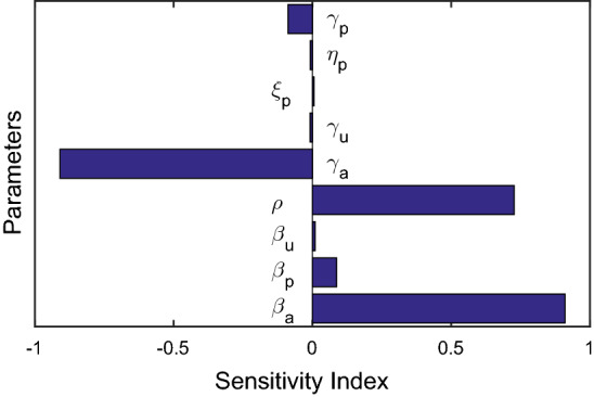
The plot represents the normalized forward sensitivity indices of the basic reproduction number $R_0$ with respect to the baseline system parameter values specified in Table 1

Optimal control problem

The control measures play an important role in mitigating the transmission of the COVID-19 dynamics. Thus, in this section we formulate an optimal control problem using $u_1(t)$ and $u_2(t)$ as time-dependent control variables corresponding to the mathematical model (1). We are mainly interested to investigate the effect of these intervention strategies on the transmission of the COVID-19 virus. We minimize the infected population and the hospitalized population by using the theory of optimal intervention strategies [53]. We performed the theoretical analysis as well as numerical illustrations to show how these control strategies make an evident on the transmission of COVID-19 pandemic and to minimize the disease burden with their implementations. The definition of the parameters and supposition leads to the model (1) which implies a coupled system of nonlinear differential equations with nine state variables, that is, S(t), E(t), A(t), P(t), U(t), D(t), I(t), H(t) and R(t). In our control problem, we implemented two control variables $u_i(t)$ $(i=1,2)$ that externally control the number of isolated or hospitalized cases and clinically ill or symptomatic infected cases over a specified time window. Now, we delineate these two control strategies and then investigate their impact on COVID-19 transmission dynamics.

To provide better treatment to the clinically ill or infected individuals

Better treatment strategy to the symptomatic infected population not only weakens the disease prevalence but also influences its development. It is very essential to the individuals to consult with a doctor if the mildly symptom is observed in this body. The individuals should not neglect by considering it as a mildly cases. Consulting to the doctors at the beginning can reduce the disease transmission, and thus, a saturated isolation rate $\frac{{ϵ}_1{u}_1(t)D}{1+{\xi }_{1}D}$ is implemented in our original model (1) where ${ϵ}_1$ represents the rate at which clinically ill cases move to the hospitals for medical treatment without neglecting the symptoms with magnitude $u_1$ and half saturation constant ${\xi }_1^{-1}$. There are different costs related to the medicines, kits, diagnosis, health protocols, etc., during the period when an individual detected with coronavirus symptoms is taken into account. Hence, we consider that the treatment intensity $u_1(t)$ as a control variable lies between 0 and 1 where 0 represents case when an individual ignores his/her mild symptoms and 1 indicates the case when an individual consults with doctor neglecting the mild symptoms.

Better treatment strategy to the isolated individuals

The disease mortality can be lower by providing proper antivirals or vaccination against novel coronavirus to the isolated or hospitalized individuals at the very beginning of infection. It influences the development of the diseases too. It is to be noted that the vaccine is accessible and given to the population who are admitted in the nursing home or hospitals in a limited amount. As the accessibility of resources associated with the medical treatments, financial crisis, disease diagnosis, etc., all the equipment is restricted. To keep this mind, we implemented intervention strategy in our original model (1) by introducing a saturated treatment rate function $\frac{{ϵ}_2{u}_2(t)I}{1+{\xi }_{2}I}$ where ${ϵ}_2$ represents the treatment rate with magnitude $u_2$ along with half saturation constant ${\xi }_2^{-1}$. Different costs related to the medicines, health problem, isolation, vaccination, medical kits, etc., at the time of medication period are need to be taken into account. Thus, we consider $u_2(t)$ as a control variable lying between 0 and 1, where 0 represents no response and 1 represents full response after the treatment.

Our main aim is to obtain the optimal treatment strategy for the clinically ill population and isolated individuals with minimum cost. To do this, we consider the admissible set for two control variables $u_1(t)$ and $u_2(t)$ defined as follows:

$$\begin{array}{c}\hfill \mathcal{U}=\{u_1(t),u_2(t):0\le u_1(t),u_2(t)\le 1,t\in [0,T]\}.\end{array}$$ 9

After introducing the controls in the original system (1), we get the following system of equations:

$$\begin{array}{cc}\hfill \frac{\mathit{dS}}{\mathit{dt}}=& -S({\beta }_p\frac{P}{N}+{\beta }_a\frac{A}{N}+{\beta }_u\frac{U}{N}),\hfill \\ \hfill \frac{\mathit{dE}}{\mathit{dt}}=& S({\beta }_p\frac{P}{N}+{\beta }_a\frac{A}{N}+{\beta }_u\frac{U}{N})-{\gamma }_{e}E,\hfill \\ \hfill \frac{\mathit{dA}}{\mathit{dt}}=& \rho {\gamma }_{e}E-{\gamma }_{a}A,\hfill \\ \hfill \frac{\mathit{dP}}{\mathit{dt}}=& (1-\rho ){\gamma }_{e}E-({\gamma }_p+{\xi }_p+{\eta }_p)P,\hfill \\ \hfill \frac{\mathit{dU}}{\mathit{dt}}=& {\xi }_{p}P-{\gamma }_{u}U,\hfill \\ \hfill \frac{\mathit{dD}}{\mathit{dt}}=& {\gamma }_{p}P-{\gamma }_{d}D-\frac{{ϵ}_1{u}_1(t)D}{1+{\xi }_{1}D},\hfill \\ \hfill \frac{\mathit{dI}}{\mathit{dt}}=& {\gamma }_{d}D-({\gamma }_i+{\xi }_i)I+\frac{{ϵ}_1{u}_1(t)D}{1+{\xi }_{1}D}-\frac{{ϵ}_2{u}_2(t)I}{1+{\xi }_{2}I},\hfill \\ \hfill \frac{\mathit{dR}}{\mathit{dt}}=& {\gamma }_{i}I+{\gamma }_{a}A+{\gamma }_{u}U+{\eta }_{p}P+\frac{{ϵ}_2{u}_2(t)I}{1+{\xi }_{2}I},\hfill \\ \hfill \frac{\mathit{dH}}{\mathit{dt}}=& {\xi }_{i}I,\hfill \end{array}$$ 10

subject to the minimize the objective functional

$$\begin{array}{cc}\hfill J(u_1(t),u_2(t))=& {\int }_0^T(c_{1}D+c_{2}I+\frac{w_1}{2}{u}_1^2+\frac{w_2}{2}{u}_2^2)dt.\hfill \end{array}$$ 11

Here, J is the total cost and at any time t, the integrand ${\displaystyle L(D,I,u_1(t),u_2(t))=c_{1}D+c_{2}I+\frac{w_1}{2}{u}_1^2+\frac{w_2}{2}{u}_2^2}$ represents the current value of the cost. The positive parameters $w_1$ and $w_2$ represent the weight constants, which balance the units of the integrands [44, 46, 54].

Existence of optimal control

In this section, the existence of optimal solution of the system (10) with objective functional (11) is verified. We assure the existence of the control pair $u_1^{\ast }$ and $u_2^{\ast }$ in

$$\begin{array}{c}\hfill \Phi =\left\{u_i,,\text{is},,\text{measurable},,,,0,\le ,u_i,\le ,1,,\text{for},,t,\in ,[0,T],,,,i,=,1,,,2\right\},\end{array}$$

which minimizes the cost functional J.

Theorem 2

There exist optimal controls $u_1^{\ast }$ and $u_2^{\ast }$ in $\Phi$ corresponding to the control problem (10) and (11) on a fixed interval [0, T].

Proof

We will use Lukes [53] results to proof the theorem. In order to ensure the existence of optimal controls, the conditions listed below must be satisfied:

1. The boundedness of the solution of the control system (10) confirms the existence of the solution of control system (10).

2. The optimal control set and the corresponding state variables are non-empty.

3. The solution of the control system (10) is bounded above by a linear function in the control as well as state variables.

The integrand in the cost functional J, ${\displaystyle L(D,I,u_1(t),u_2(t))=c_{1}D+c_{2}I+\frac{w_1}{2}{u}_1^2+\frac{w_2}{2}{u}_2^2}$ is convex on the control set $\Phi$. The exist constants $a_1,a_2>0$ and $b>0$ such tat $c_{1}D+c_{2}I+\frac{w_1}{2}{u}_1^2+\frac{w_2}{2}{u}_2^2\le a_1+a_2(|u_1{|}^2+{|u_2|}^2{)}^{q/2}$ where $a_1$ depends upon the upper bounds of D and I and $b_2=max\left\{u_1,,,u_2\right\}$. $\square$

Characterization of optimal control

Now, we need to estimate the value of optimal controls $u_1^{\ast }(t)$ and $u_2^{\ast }(t)$ such that

$$\begin{array}{cc}\hfill J(u_1^{\ast },u_2^{\ast })=& \underset{u_1,u_2\in \Phi }{min}J(u_1,u_2)\hfill \end{array}$$ 12

where

$$\begin{array}{cc}\hfill \Phi =& \left\{u_i,,\text{is},,\text{measurable},,,0,\le ,u_i,\le ,1,,\text{for},,t,\in ,[0,T],,,,i,=,1,,,2\right\}.\hfill \end{array}$$

The Lagrangian is given by

$$\begin{array}{c}\hfill L(D,I,u_1(t),u_2(t))=c_{1}D+c_{2}I+\frac{w_1}{2}{u}_1^2+\frac{w_2}{2}{u}_2^2.\end{array}$$ 13

The Hamiltonian is defined as follows:

$$\begin{array}{cc}& H(D,I,u_1,u_2,{\lambda }_1,{\lambda }_2,{\lambda }_3,{\lambda }_4,{\lambda }_5,{\lambda }_6,{\lambda }_7,{\lambda }_8,{\lambda }_9)\hfill \\ \hfill & =L(D,I,u_1(t),u_2(t))+{\lambda }_1\frac{\mathit{dS}}{\mathit{dt}}+{\lambda }_2\frac{\mathit{dE}}{\mathit{dt}}+{\lambda }_3\frac{\mathit{dA}}{\mathit{dt}}+{\lambda }_4\frac{\mathit{dP}}{\mathit{dt}}+{\lambda }_5\frac{\mathit{dU}}{\mathit{dt}}\hfill \\ \hfill & +{\lambda }_6\frac{\mathit{dD}}{\mathit{dt}}+{\lambda }_7\frac{\mathit{dI}}{\mathit{dt}}+{\lambda }_8\frac{\mathit{dR}}{\mathit{dt}}+{\lambda }_9\frac{\mathit{dH}}{\mathit{dt}}\hfill \end{array}$$ 14

where the adjoint variables can be obtained as the solution of the following system of differential equations

$$\begin{array}{cc}\hfill {\lambda }_1^{\prime }(t)=& -\frac{\partial S}{\partial t}=({\lambda }_1-{\lambda }_2)({\beta }_p\frac{P}{N}+{\beta }_a\frac{A}{N}+{\beta }_u\frac{U}{N})I,\hfill \\ \hfill {\lambda }_2^{\prime }(t)=& -\frac{\partial E}{\partial t}=({\lambda }_2-{\lambda }_4){\gamma }_e+({\lambda }_4-{\lambda }_3)\rho {\gamma }_e,\hfill \\ \hfill {\lambda }_3^{\prime }(t)=& -\frac{\partial A}{\partial t}=({\lambda }_1-{\lambda }_2){\beta }_a\frac{S}{N}+({\lambda }_3-{\lambda }_8){\gamma }_a,\hfill \\ \hfill {\lambda }_4^{\prime }(t)=& -\frac{\partial P}{\partial t}=({\lambda }_1-{\lambda }_2){\beta }_p\frac{S}{N}+({\lambda }_4-{\lambda }_6){\gamma }_p+({\lambda }_4-{\lambda }_5){\xi }_p+({\lambda }_4-{\lambda }_8){\eta }_p,\hfill \\ \hfill {\lambda }_5^{\prime }(t)=& -\frac{\partial U}{\partial t}=({\lambda }_1-{\lambda }_2){\beta }_u\frac{S}{N}+({\lambda }_5-{\lambda }_8){\gamma }_u,\hfill \\ \hfill {\lambda }_6^{\prime }(t)=& -\frac{\partial D}{\partial t}=-c_1+({\lambda }_6-{\lambda }_7){\gamma }_d+({\lambda }_6-{\lambda }_7)\frac{{ϵ}_1{u}_1}{{(1+{\xi }_{1}D)}^2},\hfill \\ \hfill {\lambda }_7^{\prime }(t)=& -\frac{\partial I}{\partial t}=-c_2+({\lambda }_7-{\lambda }_8)\frac{{ϵ}_2{u}_2}{{(1+{\xi }_{2}I)}^2}+({\lambda }_7-{\lambda }_8){\gamma }_i+({\lambda }_7-{\lambda }_9){\xi }_i,\hfill \\ \hfill {\lambda }_8^{\prime }(t)=& -\frac{\partial R}{\partial t}=0,\hfill \\ \hfill {\lambda }_9^{\prime }(t)=& -\frac{\partial H}{\partial t}=0.\hfill \end{array}$$ 15

satisfying ${\lambda }_i(T)=0$, for $i=1,2,3,\cdots ,9$, that is the transversality conditions. Now, using Pontryagin’s maximum principle [53, 54] we characterize the optimal control pair $u_1^{\ast }$ and $u_2^{\ast }$ as follows:

Theorem 3

Let $u_1^{\ast }$ and $u_2^{\ast }$ be optimal control variables and $S^{\ast },E^{\ast },A^{\ast },P^{\ast },U^{\ast },D^{\ast },I^{\ast },R^{\ast },$ and $H^{\ast }$ be corresponding optimal state variables of the system (10)-(12). Then, there exists adjoint variable $\lambda =({\lambda }_1,{\lambda }_2,{\lambda }_3,{\lambda }_4,{\lambda }_5,{\lambda }_6,{\lambda }_7,{\lambda }_8,{\lambda }_9)\in {\mathbf{R}}^9$ that satisfies the canonical equations (15) with transversality conditions ${\lambda }_i(T)=0$, for $i=1,2,3,\cdots ,9$. The corresponding optimal controls $u_1^{\ast }$ and $u_2^{\ast }$ are given as,

$$\begin{array}{c}\hfill u_1^{\ast }=min\left\{max,\left\{0,,,({\lambda }_6-{\lambda }_7),\frac{{ϵ}_{1}D}{w_1(1+{\xi }_{1}D)}\right\},,,1\right\},\end{array}$$ 16

and

$$\begin{array}{c}\hfill u_2^{\ast }=min\left\{max,\left\{0,,,({\lambda }_7-{\lambda }_8),\frac{{ϵ}_{2}I}{w_2(1+{\xi }_{2}I)}\right\},,,1\right\}.\end{array}$$ 17

Proof

Let $u_1^{\ast }$ and $u_2^{\ast }$ be the given optimal control variables and $S^{\ast },E^{\ast },A^{\ast },P^{\ast },U^{\ast },D^{\ast },I^{\ast },R^{\ast },$ and $H^{\ast }$ be corresponding optimal state variables of the system (10) which minimize the cost functional (11). Hence, by the Pontryagin’s maximum principle, there exist adjoint variables ${\lambda }_1,{\lambda }_2,{\lambda }_3,{\lambda }_4,{\lambda }_5,{\lambda }_6,{\lambda }_7,{\lambda }_8$ and ${\lambda }_9$, which satisfy canonical equations (15) with transversality conditions ${\lambda }_i(T)=0$, for $i=1,2,3,\cdots ,9$. Now, using the optimality condition, we obtain

${\displaystyle \frac{\partial H}{\partial u_1}=0}$ at $u_1=u_1^{\ast }$ and ${\displaystyle \frac{\partial H}{\partial u_2}=0}$ at $u_2=u_2^{\ast }$.

Thus, we obtain ${\displaystyle u_1^{\ast }=({\lambda }_6-{\lambda }_7)\frac{{ϵ}_{1}D}{w_1(1+{\xi }_{1}D)}}$ and ${\displaystyle u_2^{\ast }=({\lambda }_7-{\lambda }_8)\frac{{ϵ}_{2}I}{w_2(1+{\xi }_{2}I)}}$.

Hence, using the above results along with the characteristics of control set $\Phi$, we obtain

$$\begin{array}{c}\hfill u_1^{\ast }=\left\{\begin{array}{cc}\text{0,}\hfill & ({\lambda }_6-{\lambda }_7)\frac{{ϵ}_{1}D}{w_1(1+{\xi }_{1}D)}<0,\hfill \\ ({\lambda }_6-{\lambda }_7)\frac{{ϵ}_{1}D}{w_1(1+{\xi }_{1}D)},\hfill & ({\lambda }_6-{\lambda }_7)\frac{{ϵ}_{1}D}{w_1(1+{\xi }_{1}D)}\le 1,\hfill \\ \text{1,}\hfill & ({\lambda }_6-{\lambda }_7)\frac{{ϵ}_{1}D}{w_1(1+{\xi }_{1}D)}>1,\hfill \end{array}\right)\end{array}$$

and

$$\begin{array}{c}\hfill u_2^{\ast }=\left\{\begin{array}{cc}\text{0,}\hfill & ({\lambda }_6-{\lambda }_7)\frac{{ϵ}_{1}D}{w_1(1+{\xi }_{1}D)}<0,\hfill \\ ({\lambda }_6-{\lambda }_7)\frac{{ϵ}_{1}D}{w_1(1+{\xi }_{1}D)},\hfill & ({\lambda }_6-{\lambda }_7)\frac{{ϵ}_{1}D}{w_1(1+{\xi }_{1}D)}\le 1,\hfill \\ \text{1,}\hfill & ({\lambda }_6-{\lambda }_7)\frac{{ϵ}_{1}D}{w_1(1+{\xi }_{1}D)}>1,\hfill \end{array}\right)\end{array}$$

which can be equivalently written as (16) and (17). $\square$

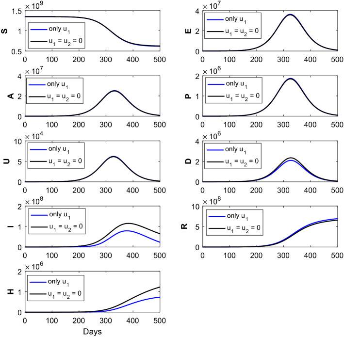
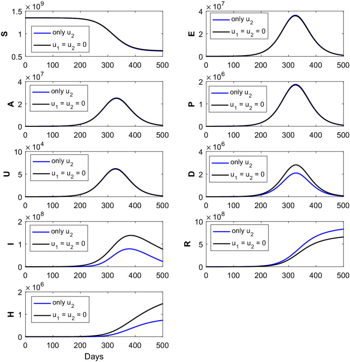
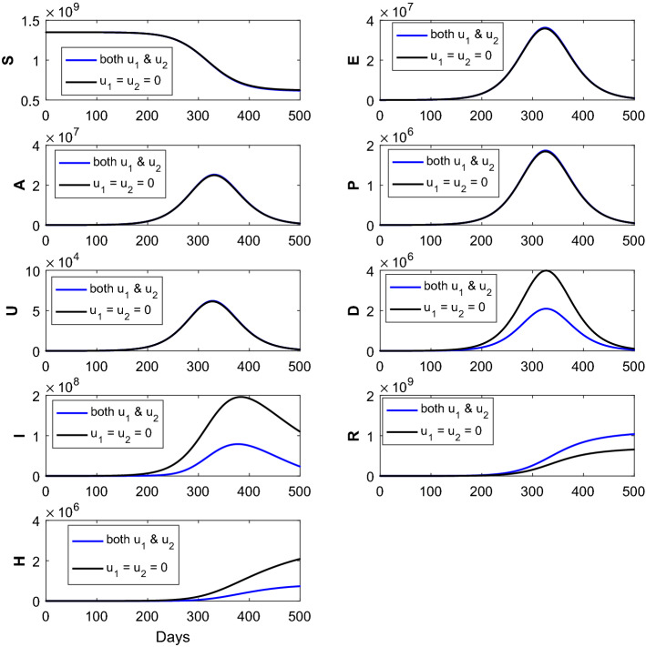
We numerically solved the control system (10) subject to the objective functional $J(u_1^{\ast },u_2^{\ast })$ with system parameter values which are listed in Table 1, and we assume the initial population as $[S(0),E(0),$  A(0),  P(0),  U(0),  $D(0),I(0),R(0),H(0)]$ = $[13.5\times {10}^8,9700,3200,50,10,03,0,0,0]$. We use forward–backward sweep method to solve the optimality system numerically. The state equations are solved forward in time and after that the adjoint state system solved backward in time using Runge–Kutta fourth-order iterative scheme. The values of the controls are updated at each iteration. The process is repeated to reach a desired convergence criteria. We have compared our model with the implementation of optimal control strategy and without administration of optimal control policy, and the variation of the state variables in the presence of optimal controls and in the absence of optimal control is shown in Figs. 3, 4 and 5. It is observed that there is no significant effect of the optimal controls for the S, E, A, P and U populations.

Fig. 3.

The figure represents the comparison of the corresponding susceptible (S), exposed (E), asymptomatic (A), pre-symptomatic (P), symptomatic undetected (U), clinically ill or symptomatic detected (D), isolated or hospitalized (I), recovered (R) and dead (H) classes without intervention strategies, with the implementation of intervention strategies (only $u_1$ control). Optimal treatment strategy (solid blue line) demonstrates reduction of the (D), (I) and (H) classes and increase in the (R) class when compared with the no controls (solid black curves). The parameter values are given in Table 1

Fig. 4.

The figure represents the comparison of the corresponding susceptible (S), exposed (E), asymptomatic (A), pre-symptomatic (P), symptomatic undetected (U), clinically ill or symptomatic detected (D), isolated or hospitalized (I), recovered (R) and dead (H) classes without intervention strategies, with the implementation of intervention strategies (only $u_2$ control). Optimal treatment strategy (solid blue line) demonstrates substantial reduction of the (D), (I) and (H) classes and substantial increment of the (R) class when compared with the no controls (solid black curves). The parameter values are given in Table 1

Fig. 5.

The figure represents the comparison of the corresponding susceptible (S), exposed (E), asymptomatic (A), pre-symptomatic (P), symptomatic undetected (U), clinically ill or symptomatic detected (D), isolated or hospitalized (I), recovered (R) and dead (H) classes without intervention strategies, with the implementation of intervention strategies (combination of the two controls $u_1$ and $u_2$). Optimal treatment strategy (solid blue line) demonstrates significant reduction of the (D), (I) and (H) classes and significant increment of the (R) class when compared with the no controls (solid black curves). The parameter values are given in Table 1

We employ two different optimal treatment strategies, namely $u_1(t)$ and $u_2(t).$ The solid black curves for epidemic (without administration of intervention strategies) are exhibited to highlight the difference from those generated via implementation of optimal treatment polices. The solid blue epidemic curves (with the implementation of single control $u_1(t)$ only) are shown the reduction of the symptomatic detected cases, isolated cases and dead population when compared with the no intervention scenario. It can also be noted that the recovered population increases after the implementation of single optimal control $u_1(t)$ when compared without administration of controls, that is, $u_1(t)=u_2(t)=0.$ Thus, the implementation of single control is better in comparison with the without control policy. The impact of the time-dependent optimal control $u_1(t)$ only [ here $u_2(t)=0]$ is shown in Fig. 3. This numerical simulation shows significant decrease in the density of I, H and D populations and significant increase in R population.

Again, the impact of the time-dependent optimal control $u_2(t)$ only [ here $u_1(t)=0]$ is plotted in Fig. 4. The solid blue epidemic curves (with the implementation of single control $u_2(t)$ only) show the reduction of the symptomatic detected cases, isolated cases and dead population when compared with the no intervention scenario (solid black curves). It can also be noted that the recovered population increases after the implementation of single optimal control $u_2(t)$ when compared without administration of controls, that is, $u_1(t)=u_2(t)=0.$ From the numerical simulation (see Fig. 4), we can infer that the effect of the optimal control $u_2(t)$ is more effective than the optimal control $u_1(t)$.

The time series Fig. 5 represents the impact of each treatment strategies on the disease state variables in the presence of the optimal control strategy and in the absence of optimal treatment strategy. These plots demonstrate the cases under no control $(u_1(t)=u_2(t)=0)$, with the combination of two different controls $(u_1(t),u_2(t))$. The solid black curves for epidemic (without implementation of intervention strategies) are shown to highlight the difference from those generated through the administration of optimal treatment polices. The solid blue epidemic curves (with the administration of the combined of two controls) exhibit the significant reduction of the symptomatic detected cases, isolated or hospitalized cases and dead individuals when compared with the no intervention strategies. The reduction of the symptomatic infected (detected) class (D) becomes maximum when the optimal controls $u_1(t)$ and $u_2(t)$ are applied simultaneously. It is worthy in mentioning that the recovered individuals (R) increased substantially when compared with the no control cases as well as the implementation of single controls $u_1(t)$ and $u_2(t).$ Implementation of the combination of two controls is better when compared with the no control policy as well as the single control policy. Thus, from the numerical simulations (Fig. 5) we can infer that the employment of intervention strategy has an effect in controlling the spread of novel coronavirus epidemic. Also, we can conclude that the combination of two controls is more effective when compared with the implementation of the single control.

The time evolution of the control variables $u_1(t)$ and $u_2(t)$ is shown in Fig. 6 with respect to the disease transmission rate $({\beta }_a)$ due to contact between susceptible and asymptomatic population. Figure 7 shows the time evolution of the control variable $u_1(t)$ with respect to the parameter ${ϵ}_1$ (left panel) and the time evolution of the control variable $u_2(t)$ with respect to the parameter ${ϵ}_2$ (right panel). The time evolution of the control variable $u_1(t)$ and $u_2(t)$ is shown in Fig. 8 with respect to the rate $({\gamma }_a)$ at which asymptomatic infected individuals become recovered.

Fig. 6.

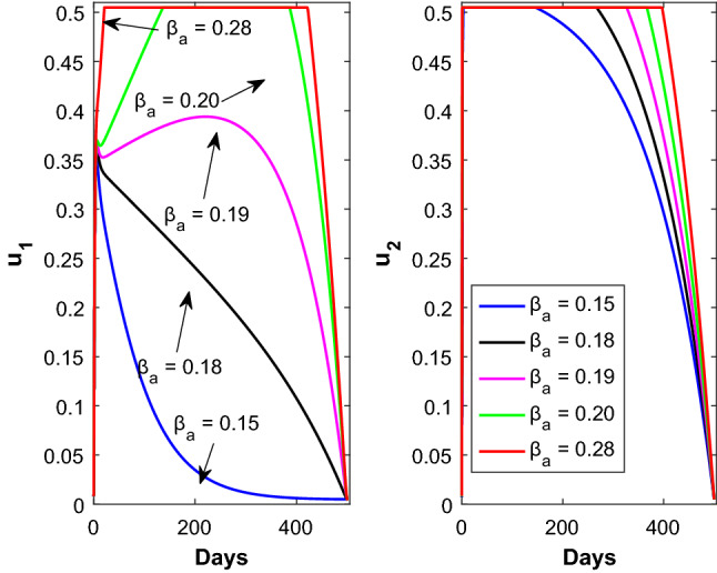
Time profile of the optimal controls $u_1(t)$ (left panel) and $u_2(t)$ (right panel) for different values of ${\beta }_a$. Rest of the parameters are defined in Table 1

Fig. 7.

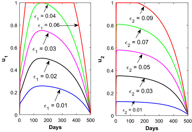
Time profile of the optimal controls $u_1(t)$ (left panel) for different values of ${ϵ}_1$ and $u_2(t)$ (right panel) for different values of ${ϵ}_2$

Fig. 8.

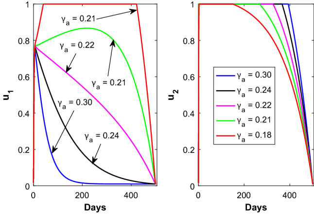
Time profile of the optimal controls $u_1(t)$ (left panel) and $u_2(t)$ (right panel) for different values of ${\gamma }_a$

We designed an analysis with only $u_1$ optimal control policies, that is, implementing of optimal control strategy on isolated or hospitalized individuals. Numerical simulations of the proposed COVID-19 model, collectively SEAPUDIRH, have been shown with the application of only $u_1$ optimal control and without implementation optimal control in Fig. 3. Implementation of only $u_1$ control decreases the symptomatic detected individuals (D), isolated or hospitalized population (I), dead cases (H) and consequently the recovered class (R) has been increased. More people become recovered, and less number of people become infected after the successful implementation of only $u_1$ optimal control. Also, the number of death cases decreased after the introduction of only $u_1$ optimal control.

Next we implement the single optimal control $u_2$ for the saturated treatment rate with $u_1=0$. Here, the value of $u_2$ lies between 0 and 1, where 0 indicates no response for COVID-19 medical treatment, while 1 indicates full response for COVID-19 medical treatment. Numerical simulation of the proposed COVID-19 model, collectively SEAPUDIRH, has been shown with only $u_2$ optimal control and without implementation of optimal control in Fig. 4. Implementation of only $u_2$ optimal control decreases the symptomatic detected (D) cases, isolated or hospitalized (I) cases, dead classes (H) and increases the number of recovered (R) population. More population become recovered, and less number of population become infected after the successful implementation of only $u_2$ optimal control. Here, also the number of death cases reduced after the implementation of only $u_2$ optimal control.

Now, we implement both the optimal controls $u_1$ and $u_2$ simultaneously in our proposed SEAPUDIRH model. Numerical solution of the proposed COVID-19 model, collectively SEAPUDIRH, is shown with both $u_1$ and $u_2$ optimal controls in Fig. 5. Significant decrease in the clinically ill or symptomatic detected (D) cases, isolated or hospitalized (I) individuals, dead classes (H) is observed and significantly increases the recovered (R) individuals. The number of clinically ill or symptomatic detected (D), isolated (I), dead (H) classes becomes less, while the optimal controls $u_1$ and $u_2$ are applied simultaneously when compared to the implementation of single optimal controls.

Numerical simulations

In this section, we performed some numerical illustrations for the COVID-19 pandemic in India based on the SEAPUDIRH model system (1). We estimated the SEAPUDIRH model parameters based on the daily observed COVID-19 cases, cumulative number of COVID-19 cases and the dead cases due to SARS-CoV-2 virus infection, for the time period March 01, 2020, to August 15, 2020. The data were collected from the WHO situation report [2]. We estimated six parameter values, namely ${\beta }_p$, ${\beta }_u$, ${\beta }_a$, $\rho$, ${\gamma }_a$ and ${\gamma }_p$ among 13 system parameters. The estimated value of those six system parameters is listed in Table 1. Based on the estimated model parameters and other parameters, we performed short-term prediction of the epidemic. We also performed some mathematical analysis to get an idea about the basic reproduction number $R_0$. We also showed that our system is asymptotically stable for $R_0<1$.

Preliminary insight from COVID-19 observed data

First, we perform a simple mathematical analysis that can be endeavored to obtain some insight into the COVID-19 pandemic and to generate iterative time-lag maps. The motivation is to build a relationship between some individuals at time (in days) $n+k$ and the same individuals at day n, corresponding to the time lag of k days. Thus, we have investigated the relation between the populations of ${(t+n)}^{\mathit{th}}$ and $t^{\mathit{th}}$ days for the daily new COVID-19 infection cases and daily new deaths due to COVID-19 infection with a time lag of t days. Now considering $n=1$, we have graphically shown the $t^{\mathit{th}}$ days population along horizontal axis and ${(t+1)}^{\mathit{th}}$ days population along the vertical axis (see Fig. 9). Both the populations follow the power law

$$\begin{array}{cc}\hfill X_{t+1}=& a{X_t}^b.\hfill \end{array}$$ 18

The values of the parameters a and b are 1.192 and 0.9842, respectively, for the daily new COVID-19 cases (D) with coefficient of determination $(R^2)$ = 0.9928. Also, we consider the values of the parameters a and b are 1.821 and 0.8954, respectively, for the daily new deaths (H) with coefficient of determination $(R^2)$ = 0.8950.

Fig. 9.

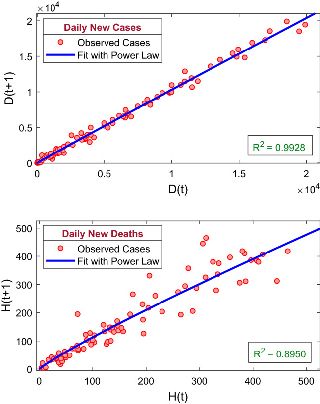
The figure represents the recurrence plots for the daily new COVID-19 cases and the daily new deaths due to COVID-19 infection. The best fit of the power law of the kind (18) is shown by solid blue curve. The coefficient of determination $(R^2)$ for the daily new COVID-19 cases is 0.9928, and the coefficient of determination $(R^2)$ for the daily new deaths is 0.8950. The best fit curves of the power law are increasing for both the populations

Model calibration

We have calibrated our proposed COVID-19 model system (1) with the daily observed COVID-19 infection cases, cumulative number of COVID-19 cases as well as the number of daily deaths due to COVID-19 infection. The data of daily new COVID-19 infection cases, cumulative number of COVID-19 infection cases, daily deaths and cumulative number of deaths due to COVID-19 infection in India were obtained from the situation report of World Health Organization (https://www.who.int) [2]. First COVID-19 cases have been observed in India on January 30, 2020, but March 01, 2020, onward, the daily new COVID-19 infection cases were reported continuously. Hence, we have collected the COVID-19 data from March 01, 2020, to August 15, 2020. Model simulation depends on both the system parameter values and the initial population sizes. As the population in India is $13.5\times {10}^8$ and the 3 persons were infected by COVID-19 as on March 01, 2020, we have considered the initial population sizes as $[S(0),E(0),A(0),P(0),U(0),D(0),I(0),R(0),H(0)]$ = $[13.5\times {10}^8,9700,3200,50,10,03,0,0,0]$ and varied the system parameter values to fit with the observed data. The model simulations were fitted with the observed daily new COVID-19 cases, cumulative number of COVID-19 cases as well as daily deaths due to COVID-19 infection, using the least square method by minimizing the sum of errors. Six model parameters, namely ${\beta }_a$, ${\beta }_p$, ${\beta }_u$, $\rho$, ${\gamma }_a$ and ${\gamma }_p$, have been estimated by this least square method out of the thirteen system parameters [50]. The value of the estimated parameters is listed in Table 1, and the best fitted curves are shown in Fig. 10. The daily new COVID-19 infection cases, cumulative number of COVID-19 cases and cumulative number of deaths have shown in first, second and third row, respectively. Filled red circles are the observed cases, and the blue curves are best fitted model simulation. Our SEAPUDIRH model system (1) nicely captured the increasing trend in all the populations. To compute the accuracy of model simulation, we have computed the root-mean-square error $(E_{\mathit{RMSE}})$ and mean absolute Error $(E_{\mathit{MAE}})$, which can be defined as follows:

$$\begin{array}{cc}\hfill E_{\mathit{RMSE}}=& \sqrt{\frac{{\Sigma }_{i=1}^n{(R(i)-M(i))}^2}{n}},\hfill \\ \hfill E_{\mathit{MAE}}=& \frac{{\Sigma }_{i=1}^n|R(i)-M(i)|}{n},\hfill \end{array}$$

where R(i) represents the observed COVID-19 infection cases, M(i) represents the model simulation on the $i^{\mathit{th}}$ day, and $n=168$ is the sample size of the observed COVID-19 data. The values of $E_{\mathit{RMSE}}$ and $E_{\mathit{MAE}}$ are 3266.6 and 2204.0, respectively.

Fig. 10.

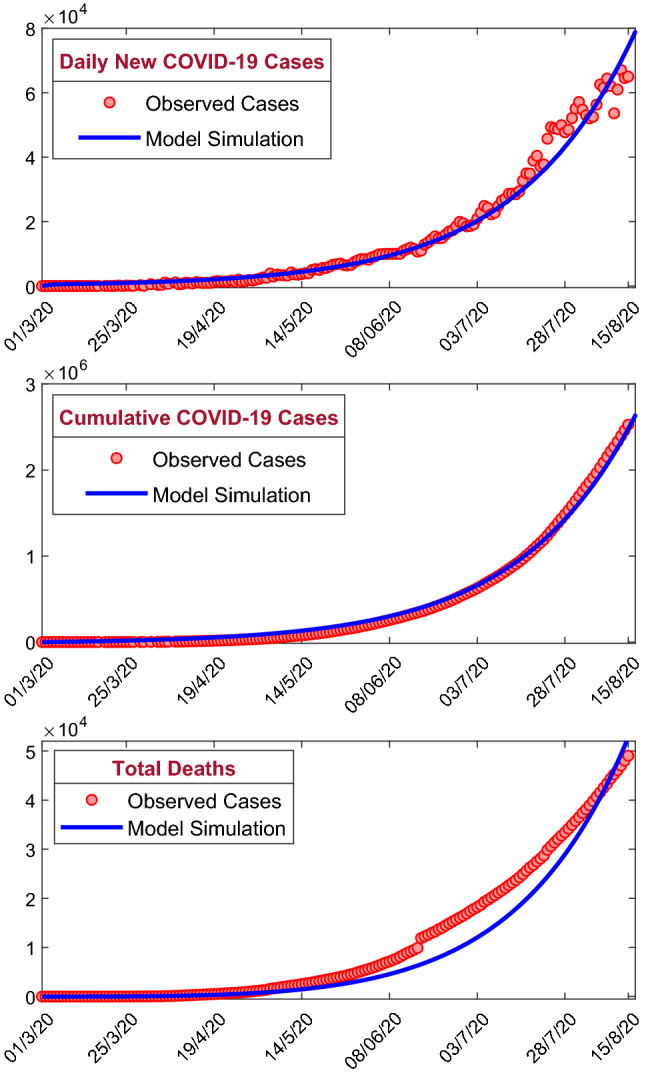
The figure shows the model simulations fitted with the observed daily new COVID-19 cases, cumulative confirmed COVID-19 cases and cumulative deaths due to COVID-19 infection in India. Observed cases are shown by the solid red circle, and the best fitting curve for the SEAPUDIRH Model system (1) is shown by blue curve. The first row represents the daily new COVID-19 cases, the second row represents the cumulative number of confirmed COVID-19 cases, and the third row represents the cumulative number of deaths due to COVID-19 infection. The initial values are used to solve the system of ordinary differential equations $[S(0),E(0),A(0),P(0),U(0),D(0),I(0),R(0),H(0)]$ = $[13.5\times {10}^8,9700,3200,50,10,03,0,0,0]$. The estimated parameter values are listed in Table 1

Impact of basic reproduction number $R_0$

An important identifier for the transmissibility of infectious diseases such as SARS-CoV-2 virus is the basic reproduction number $R_0$, which can be defined as the average number of secondary infections created by a single infected person, in a population whose all members are uninfected or susceptible. The numeric value of the basic reproduction number, $R_0$, is computed using the estimated system parameter values, and the system parameter values are listed in Table 1, and for our proposed SEAPUDIRH model, we obtained $R_0=1.4376$, which shows the substantial outbreak of COVID-19 in India.

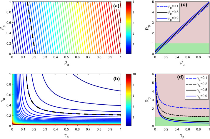
Figure 11a represents the basic reproduction number $(R_0)$ of the SEAPUDIRH system (1) with respect to ${\beta }_a$ (contact rate between susceptible and asymptomatic) and ${\beta }_p$ (contact between susceptible and pre-symptomatic). The value of $R_0$ increases if any one of the parameters ${\beta }_a$ or ${\beta }_p$ increases. The disease-free equilibrium point of the model system (1) is asymptotically stable for $R_0<1$, and for lower values of ${\beta }_a$ or ${\beta }_p$, the reproduction number $R_0$ is less than unity. Thus, the coronavirus outbreak in India can be controlled by reducing contact rate between the individuals, which can be done by maintaining social distancing and contact tracing. Figure 11c shows that if both ${\beta }_a$ and ${\beta }_p$ increase, then the value of $R_0$ will also increase significantly.

Fig. 11.

The figure shows the basic reproduction number $R_0$ of the system (1) in terms of a ${\beta }_a$ and ${\beta }_p$, b ${\gamma }_p$ and ${\gamma }_a$, c ${\beta }_a$ and d ${\gamma }_p$. In the figures (c) and (d), green shading region indicates $R_0<1$ and red shading region indicates $R_0>1$. Parameters value are ${\beta }_p=0.3649$, ${\beta }_a=0.2788$, ${\beta }_u=0.369$, ${\gamma }_e=0.15$, $\rho =0.67$, ${\gamma }_a=0.1428$, ${\gamma }_p=0.93575$, ${\xi }_p=0.01425$, ${\eta }_p=0.0112$, ${\gamma }_u=0.428$, ${\gamma }_d=0.736$, ${\gamma }_i=0.008$ and ${\xi }_i=0.000037$. The black dashed contours in the figures (a) and (b) are the contours for $R_0=1$

Figure 11b represents the basic reproduction number $(R_0)$ of the SEAPUDIRH system (1) with respect to ${\gamma }_p$ (the rate at which pre-symptomatic infected person becomes symptomatic detected) and ${\gamma }_a$ (the rate at which asymptomatic infected individuals become recovered). For larger value of ${\gamma }_p$, the value of $R_0$ becomes less than 1 if ${\gamma }_a$ increases; that is, if the rate of conversion of pre-symptomatic infected individuals (P) to symptomatic detected (D) is higher, then higher rate of recovery makes the disease-free steady-state stable. But for a lower value of ${\gamma }_p$, if ${\gamma }_a$ increases, then the value of $R_0$ remains greater than unity, that is, for lower rate of conversion from pre-symptomatic infected individuals (P) to symptomatic detected (D) will not ensure the stability of the disease-free equilibrium even if the rate of recovery is high enough. This suggests that, to make the system disease free, identification of pre-symptomatic infected individuals (P) is utmost important which can be done by increasing the number of COVID-19 test. Figure 11d represents that for higher value of ${\gamma }_a$ the value of $R_0$ becomes less than one if ${\gamma }_p$ increases and the disease-free steady state becomes stable. Thus, to mitigate the coronavirus disease from the system, the value of ${\gamma }_a$ need to increase, which can be done by increasing the number of COVID-19 test.

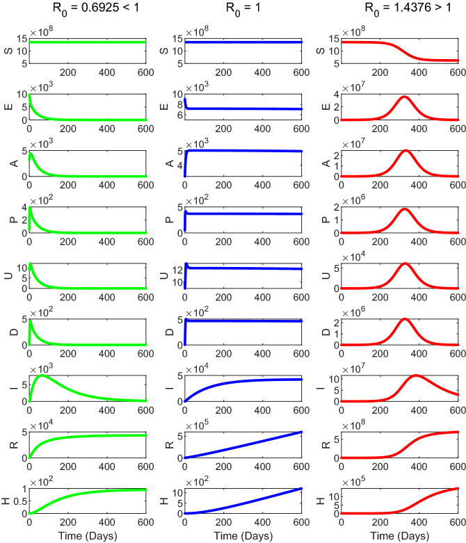
The time evolution of the proposed mathematical model system (1) is shown in Fig. 12. The system parameters are chosen in such a way that $R_0<1$ for the first column, $R_0=1$ for the second column and $R_0>1$ for the third column of Fig. 12. The time series solution in the first column of Fig. 12 shows that the disease-free equilibrium point of the system (1) is stable when $R_0<1$. The third column in Fig. 12 shows that the endemic equilibrium point of the system (1) is stable when $R_0>1$. The second column shows the time evolution of the system (1) for $R_0=1$, which indicates that there is no exponential growth of the number of active cases with time. However, it can still be growing at a slower than exponential rate, for example, linearly or logarithmically. Thus, we observed from our numerical simulation that the model system (1) is locally asymptotically stable around the disease-free equilibrium if $R_0<1$ and the endemic equilibrium point is stable if $R_0>1$.

Fig. 12.

The figure represents the numerical simulation of the system (1) for $R_0<1$ (first column), $R_0=1$ (second column) and $R_0>1$ (third column). Parameter values are specified in Table 1

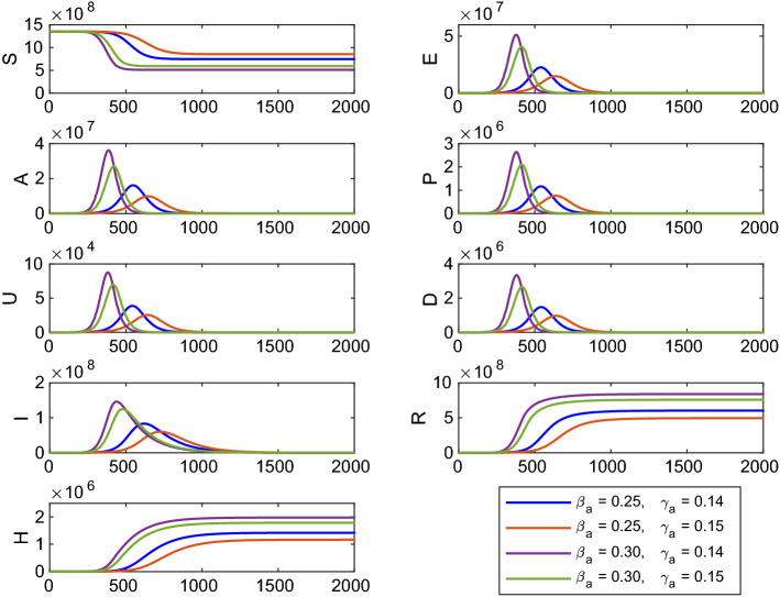
Sensitivity analysis of basic reproduction number $R_0$ shows that the system parameters ${\beta }_a$, ${\gamma }_a$ and $\rho$ are most sensitive with reference to $R_0$. The time evolution of the system (1) is shown in Fig. 13 for different values of the system parameters ${\beta }_a$ and ${\gamma }_a$. Other system parameters for the numerical simulation are same as in Table 1. Here, $R_0=1.3259$ for ${\beta }_a=0.25$, ${\gamma }_a=0.14$; $R_0=1.2462$ for ${\beta }_a=0.25$, ${\gamma }_a=0.15$; $R_0=1.5652$ for ${\beta }_a=0.30$, ${\gamma }_a=0.14$; $R_0=1.4695$ for ${\beta }_a=0.30$, ${\gamma }_a=0.15$. Thus, the number of infected cases is more for ${\beta }_a=0.25$ (or ${\beta }_a=0.30$) but lower value of ${\gamma }_a=0.14$. Therefore, if the disease transmission rate (${\beta }_a$) (contact between susceptible and asymptomatic individuals) remains constant but the rate (${\gamma }_a$) at which asymptomatic infected individuals become recovered is decreased, then the number of infected cases will increase with time.

Fig. 13.

Time profile of the populations of the system (1) for different values of ${\beta }_a$ and ${\gamma }_a$. Other parameters are same as in Table 1

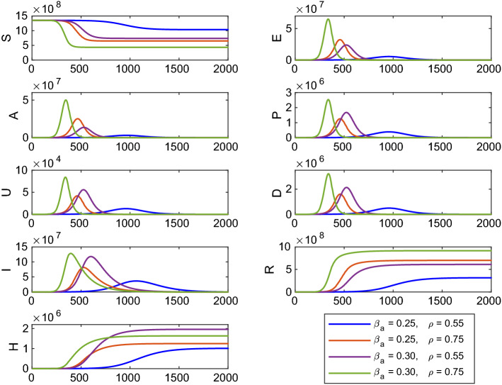
Again the time evolution of the model system (1) is shown in Fig. 14 for different values of the system parameters ${\beta }_a$ and $\rho$. Other system parameters for the numerical simulation are same as in Table 1. Here, $R_0=1.1395$ for ${\beta }_a=0.25$, ${\gamma }_a=0.55$; $R_0=1.4111$ for ${\beta }_a=0.25$, ${\gamma }_a=0.75$; $R_0=1.3320$ for ${\beta }_a=0.30$, ${\gamma }_a=0.55$; $R_0=1.6737$ for ${\beta }_a=0.30$, ${\gamma }_a=0.75$. Here, the number of infected cases become more for ${\beta }_a=0.25$ (or ${\beta }_a=0.30$) and for the higher value of $\rho =0.75$. Thus, if the disease transmission rate (${\beta }_a$) (contact between susceptible and asymptomatic individuals) remains constant but fraction of asymptomatic carriers ($\rho$) is increased, then the number of infected cases will also increase. In this scenario, we noticed that the most effective parameter of the system (1) is the disease transmission rate (${\beta }_a$) and has an impact in controlling the basic reproduction number $R_0$.

Fig. 14.

Time profile of the populations of the system (1) for different values of ${\beta }_a$ and $\rho$. Other parameters are same as in Table 1

Short-term prediction

As on August 15, 2020, the total number of COVID-19 infected cases is 25,26,192 and 49,036 people died due to COVID-19 infection. To control the transmission of the COVID-19 disease, Govt. of India has implemented nationwide four phases of lockdown and two phases of unlock. Due to the absence of licensed vaccine, antivirals and any therapeutics, Govt. is taking lockdown and unlock policies to control the community level transmission. Infection disease mathematical modeling provides an efficient prediction of the COVID-19 outbreak for short time duration. But, due to an inaccurate of data, the prediction based on the estimated data and model assumptions may not always be true. This predictions are essential to take necessary administrative strategies by the government and some other non-governmental agencies. The second phase of unlock starts from July 01, 2020, and the second phase unlock will continue up to July 31, 2020. In this study, we have considered COVID-19 data from March 01, 2020, to August 15, 2020, and our model provides short-term prediction for 21 days from August 16, 2020, to September 05, 2020 (see Fig. 15 for short-term prediction). The black dashed curve in Fig. 15 is the predicted cases, first row predicts the daily new COVID-19 cases, second row predicts the cumulative number of confirmed COVID-19 cases, and third row predicts the total deaths due to COVID-19 infection in India. Our model predicts 138,744 daily new cases, 4,676,105 cumulative cases and total 103,729 deaths on September 05, 2020. This prediction gives us an estimation of the COVID-19 outbreak in India. This prediction highly depends on the system parameter values and the initial population sizes. If the administrative strategies changed or effective vaccine or therapeutics introduced, the prediction may differ from the actual cases.

Fig. 15.

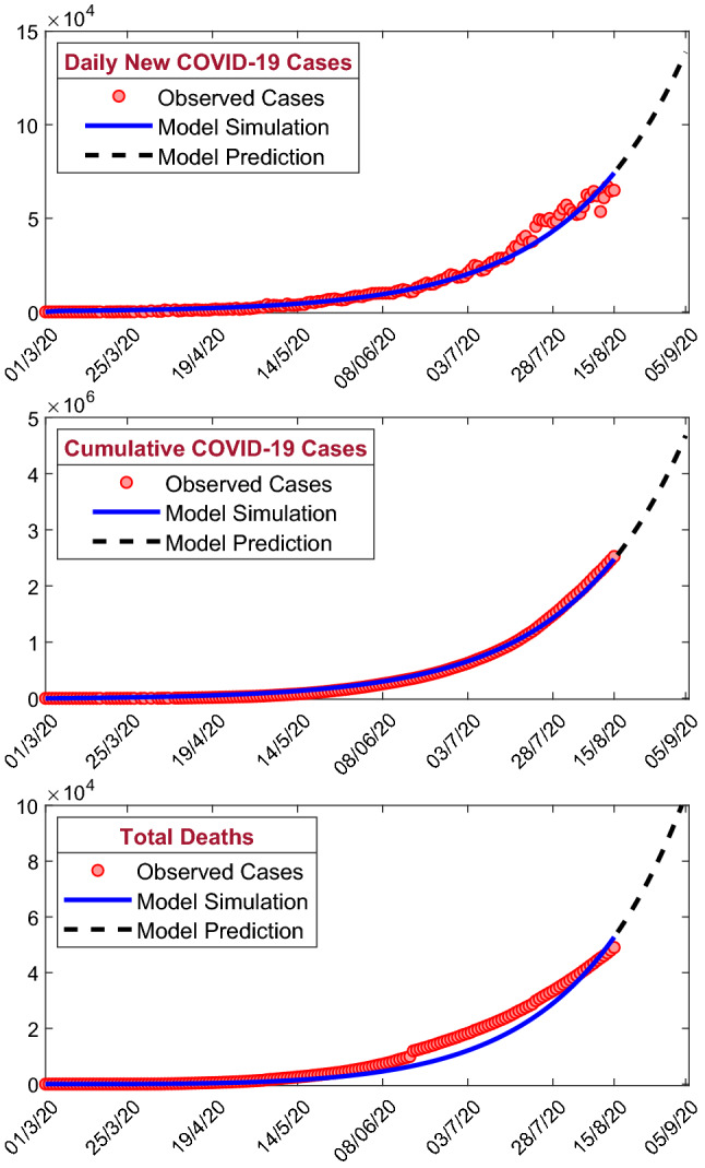
The figure represents the short-term prediction (21 days from July 01, 2020, to July 23, 2020) of the model (1) for the daily new COVID-19 cases (first row), the cumulative number of COVID-19 cases (second row) and the cumulative number of deaths due to COVID-19 infection (third row) in India. Our model predicts increasing trends for all the classes

Conclusion

In this article, we have analyzed the COVID-19 pandemic data in India made available to the researchers by the WHO situation report [2] and referring to the time period March 01, 2020, to August 15, 2020. Everyday the total number of daily confirmed cases rises with more than 2,500 reported from several states and union territories in India. This is a worrying situation as with a second most populated country in the world, and within few days, India will enter in community-wide transmission of COVID-19 epidemic. Due to the absence of any effective treatment, antivirals or licensed vaccine and with an incomplete understanding of epidemiological traits, predictive compartmental mathematical models can aid in understanding of both the disease spread and its control [13, 17].

In our present study, we have formulated and analyzed a compartmental epidemiological model of SARS-CoV-2 viruses to control and forecast the pandemic. We have computed the basic reproduction number $R_0$ to get an idea under what condition the disease will be die out or spread into the population. We also showed that whenever $R_0<1$, the disease-free steady state will be asymptotically stable. In our proposed model, we have considered the transmission variability between asymptomatic and pre-symptomatic infected persons to better understand the dynamics of the COVID-19 epidemic [18]. Also, we have investigated the sensitivity indices of the threshold quantity $R_0$ and obtained that the disease transmission rate is the most sensitive system parameter, which has a positive influenced on the basic reproduction number $R_0$.

We have calibrated our proposed mathematical model to fit the daily confirmed new COVID-19 cases, cumulative number of confirmed COVID-19 cases and the cases of daily new deaths due to COVID-19 infection of India. Six model parameters are estimated from the best curve fitting of our SEAPUDIRH model. Using the estimated system parameter values, we then obtain the basic reproduction number $R_0=1.4376$, which shows the substantial outbreak of COVID-19 pandemic in India. The policymakers and health care agencies should focus on the successful implementation of control mechanisms to mitigate the burden of the COVID-19 diseases. From the contour plot (see Fig. 11), it can be concluded that to mitigate the disease transmission must maintain the social distancing and contact tracing by implementation of nationwide lockdown, closing of educational institutions, etc.

The calibrated model is then used for short-term prediction of India for the time period August 16, 2020, to September 05, 2020 (see Fig. 15). However, the increasing pattern of daily newly COVID-19 cases, cumulative number of COVID-19 cases and the deaths cases of COVID-19 is well captured by our model for India. From the short-term prediction, we can conclude that 138,744 daily new confirmed cases, 4,676,105 cumulative number of confirmed cases and the total 103,729 deaths on September 05, 2020. It is worthy to mention that here we can predict the nature of the SARS-CoV-2 for the short-term period as the Govt. strategy can be changed in time to time resulting in the interrelated changes in the associated system parameters of our SEAPUDIRH model.

Moreover, we have modified our SEAPUDIRH model system by implementation of the theory of optimal control. Implementation of intervention strategies helps to mitigate the novel coronavirus burden. To study the impact of non-pharmaceutical and pharmaceutical intervention strategies and to reduce/stop the community transmission of the novel coronavirus, we implemented two different control measures, namely $u_1(t)$ and $u_2(t)$. Analytically, we investigated the existence of the optimal control functions. Furthermore, to mitigate the clinically ill populations and to give the better treatments for isolated or hospitalized individuals and to minimize the cost of the control functions, an objective functional $J(u_1(t),u_2(t))$ has been formulated and interpreted with the aid of Pontryagin’s maximum principle.

The behavioral changes in the susceptible population alter with time, and to prevent or limit the rate of interaction between susceptible (S) and isolated (J) individuals, we put the external effort as an intervention strategy. Also, the clinically ill or infected individuals become aware about the coronavirus disease fatality and consult with medical officers or admit to the hospitals or nursing home if the symptom occurs and thus we use the control $u_1(t)$ that alters the fraction of infected cases. Again, we apply the controlling effort $u_2(t)$ that taking into account the cost regarding medical treatments, use of test kits and life-saving medicines is provided to the hospitalized or isolated individuals. Thus, we considered all these two control policies in our proposed model.

Finally, through an extensive numerical illustrations, we conclude certain observations. Numerical solutions are demonstrated in Fig. 3 that the control strategy represents clinically ill or infected cases $u_1(t)$ efforts with its intensity for quite a long period of time and then it reduces. Later on, the control indicates better treatment strategy for isolated individuals $u_2(t)$ efforts with high magnitude nearly about 300 days following a reduction at a later stage, though this magnitude is higher than the magnitude of without control strategy. From the extensive numerical simulations (see Fig. 5), we can conclude that the implementation of intervention strategy has an important effect in controlling the spread of novel coronavirus pandemic. Also, we can conclude that the combination of two controls is more effective when compared with the implementation of the single control as well as without control. Thus, introducing the combination of two control strategies may help to reduce the spread of novel coronavirus disease at this present pandemic scenario. We plan to expand our COVID-19 modeling by introducing vaccination and the effect of environmental contamination. Most probably, this COVID-19 epidemic will remain in the human population for many years, so the changes we see in public health services and in human habits have to go on over time.

Author Contributions

The authors contributed equally to this work. All authors read and approved the final manuscript.

Data Availability Statement

All data supporting the findings of this study are in the paper and available from the corresponding author on reasonable request. This manuscript has associated data in a data repository. [Authors comment: WHO Situation Report, Coronavirus disease (COVID-19). https://www.who.int.]

Declarations

Conflict of interest

The authors declare that they have no conflict of interest.

References

- 1.Kucharski AJ, Russell TW, Diamond C, Liu Y, Edmunds J, Funk S, Eggo RM. Early dynamics of transmission and control of COVID-19: a mathematical modelling study. Lancet Infect Dis. 2020;20(5):553–558. doi: 10.1016/S1473-3099(20)30144-4. [DOI] [PMC free article] [PubMed] [Google Scholar]
- 2.WHO Situation Report, Coronavirus disease 2019 (COVID-19). (2021). https://www.who.int/publications/m/item/weekly-epidemiological-update-on-covid-19---23-march-2021
- 3.Gralinski LE, Menachery VD. Return of the coronavirus: 2019-nCoV. Viruses. 2020;12(2):135. doi: 10.3390/v12020135. [DOI] [PMC free article] [PubMed] [Google Scholar]
- 4.BBC News, https://www.bbc.com/news/world-52114829 (Retrieved on April 01, 2020)
- 5.N.M. Ferguson, D. Laydon, G. Nedjati-Gilani, N. Imai, et al. Impact of non-pharmaceutical interventions (NPIs) to reduce COVID-19 mortality and healthcare demand. Imperial College COVID-19 Response Team 1–20 (2020)
- 6.India Today. https://www.indiatoday.in/india/story/kerala-reports-first-confirmed-novel-coronavirus-case-in-india-1641593-2020-01-30. (Retrived on January 30 2020)
- 7.Pulla P. Covid-19: India imposes lockdown for 21 days and cases rise. BMJ. 2020 doi: 10.1136/bmj.m1251. [DOI] [PubMed] [Google Scholar]
- 8.Kermack WO, McKendrick AG. A contribution to the mathematical theory of epidemics. Proc. R. Soc. Lond. 1927;115:700–721. [Google Scholar]
- 9.Tang B, Wang X, Li Q, Bragazzi NL, Tang S, Xiao Y, Wu J. Estimation of the transmission risk of the 2019-ncov and its implication for public health interventions. J. Clin. Med. 2020;9(2):462. doi: 10.3390/jcm9020462. [DOI] [PMC free article] [PubMed] [Google Scholar]
- 10.S. Khajanchi, K. Sarkar, J. Mondal, Dynamics of the COVID-19 pandemic in India. arXiv:2005.06286 (2020)
- 11.Sarkar K, Khajanchi S, Nieto JJ. Modeling and forecasting the COVID-19 pandemic in India. Chaos Soliton Fract. 2020;139:110049. doi: 10.1016/j.chaos.2020.110049. [DOI] [PMC free article] [PubMed] [Google Scholar]
- 12.Wu JT, Leung K, Bushman M, Kishore N, Niehus R, de Salazar PM, Cowling BJ, Lipsitch M, Leung GM. Estimating clinical severity of COVID-19 from the transmission dynamics in Wuhan. China. Nat Med. 2020;26:506–510. doi: 10.1038/s41591-020-0822-7. [DOI] [PMC free article] [PubMed] [Google Scholar]
- 13.Giordano G, Blanchini F, Bruno R, Colaneri P, Di Filippo A, Di Matteo A, Colaneri M. Modelling the COVID-19 epidemic and implementation of population-wide interventions in Italy. Nat. Med. 2020;26:855–860. doi: 10.1038/s41591-020-0883-7. [DOI] [PMC free article] [PubMed] [Google Scholar]
- 14.A. Das, A. Dhar, S. Goyal, A. Kundu, Covid-19: analysis of a modified SEIR model, a comparison of different intervention strategies and projections for India. arXiv:2005.11511 (2020) [DOI] [PMC free article] [PubMed]
- 15.Khajanchi S, Sarkar K. Forecasting the daily and cumulative number of cases for the COVID-19 pandemic in India. Chaos. 2020;30:071101. doi: 10.1063/5.0016240. [DOI] [PMC free article] [PubMed] [Google Scholar]
- 16.S. Shekatkar, B. Pujari, M. Arjunwadkar, et al., INDSCI-SIM: A state-level epidemiological model for India. https://indscicov.in/indscisim (2020)
- 17.Gatto M, Bertuzzo E, Mari L, Miccoli S, Carraro L, Casagrandi R, Rinaldo A. Spread and dynamics of the COVID-19 epidemic in Italy: Effects of emergency containment measures. PNAS. 2020;117(19):10484–10491. doi: 10.1073/pnas.2004978117. [DOI] [PMC free article] [PubMed] [Google Scholar]
- 18.Leung KY, Trapman P, Britton T. Who is the infector? Epidemic models with symptomatic and asymptomatic cases. Math. Biosci. 2018;301:190–198. doi: 10.1016/j.mbs.2018.04.002. [DOI] [PubMed] [Google Scholar]
- 19.S. Agrawal, S. Bhandari, A. Bhattacharjee, A. Deo, A, et al., COVID-19 Epidemic: Unlocking the lockdown in India (working paper). IISc-TIFR Technical Report, https://covid19.iisc.ac.in/wp-content/uploads/2020/04/Report-1-20200419-UnlockingTheLockdownInIndia.pdf (2020)
- 20.J. Venkateswaran, O. Damani, Effectiveness of Testing, Tracing, Social Distancing and Hygiene in Tackling Covid-19 in India: A System Dynamics Model. arXiv:2004.08859 (2020)
- 21.Khajanchi S, Das DK, Kar TK. Dynamics of tuberculosis transmission with exogenous reinfections and endogenous reactivations. Phys. A. 2018;497:52–71. [Google Scholar]
- 22.Khan MA, Atangana A. Modeling the dynamics of novel coronavirus (2019-nCov) with fractional derivative. Alex. Eng. J. 2020;59(4):2379–2389. [Google Scholar]
- 23.Atangana A. Modelling the spread of COVID-19 with new fractal-fractional operators: Can the lockdown save mankind before vaccination? Chaos, Solitons Fractals. 2020;136:109860. doi: 10.1016/j.chaos.2020.109860. [DOI] [PMC free article] [PubMed] [Google Scholar]
- 24.Anderson RM, May RM. Infectious diseases of humans. London: Oxford University Press; 1991. [Google Scholar]
- 25.Metcalf CJE, Morris DH, Park SW. Mathematical models to guide pandemic response. Science. 2020;369:368–369. doi: 10.1126/science.abd1668. [DOI] [PubMed] [Google Scholar]
- 26.Lopez L, Rodo X. The end of social confinement and COVID-19 re-mergence risk. Nat. Hum. Behav. 2020;4:746–755. doi: 10.1038/s41562-020-0908-8. [DOI] [PubMed] [Google Scholar]
- 27.Hoertel N, et al. A stochastic agent-based model of the SARS-CoV-2 epidemic in France. Nat. Med. 2020;26:1417–1421. doi: 10.1038/s41591-020-1001-6. [DOI] [PubMed] [Google Scholar]
- 28.Kissler SM, Tedijanto C, Goldstein E, Grad YH, Lipsitch M. Projecting the transmission dynamics of SARS-CoV-2 through the postpandemic period. Science. 2020;368:860–868. doi: 10.1126/science.abb5793. [DOI] [PMC free article] [PubMed] [Google Scholar]
- 29.Easwaramoorthy D, Gowrisankar A, Manimaran A, et al. An exploration of fractal-based prognostic model and comparative analysis for second wave of COVID-19 diffusion. Nonlinear Dyn. 2021;106:1375–1395. doi: 10.1007/s11071-021-06865-7. [DOI] [PMC free article] [PubMed] [Google Scholar]
- 30.Kavitha C, Gowrisankar A, Banerjee S. The second and third waves in India: when will the pandemic be culminated? Eur. Phys. J. Plus. 2021;136:596. doi: 10.1140/epjp/s13360-021-01586-7. [DOI] [PMC free article] [PubMed] [Google Scholar]
- 31.Nazarimehr F, Pham VT, Kapitaniak T. Prediction of bifurcations by varying critical parameters of COVID-19. Nonlinear Dyn. 2020;101(3):1681–1692. doi: 10.1007/s11071-020-05749-6. [DOI] [PMC free article] [PubMed] [Google Scholar]
- 32.Ghosh S, Senapati A, Mishra A, Chattopadhyay J, Dana SK, Hens C, Ghosh D. Reservoir computing on epidemic spreading: A case study on COVID-19 cases. Phys. Rev. E. 2021;104:014308. doi: 10.1103/PhysRevE.104.014308. [DOI] [PubMed] [Google Scholar]
- 33.Weitz JS, Beckett SJ, Coenen AR. Modeling shield immunity to reduce COVID-19 epidemic spread. Nat. Med. 2020;26(6):849–854. doi: 10.1038/s41591-020-0895-3. [DOI] [PMC free article] [PubMed] [Google Scholar]
- 34.Nadim SK, Chattopadhyay J. Occurrence of backward bifurcation and prediction of disease transmission with imperfect lockdown: A case study on COVID-19. Chaos Soliton Fract. 2020;140:110163. doi: 10.1016/j.chaos.2020.110163. [DOI] [PMC free article] [PubMed] [Google Scholar]
- 35.Mandal M, Jana S, Nandi SK, Khatua A, Adak S, Kar TK. A model based study on the dynamics of COVID-19: Prediction and control. Chaos Soliton Fract. 2020;136:109889. doi: 10.1016/j.chaos.2020.109889. [DOI] [PMC free article] [PubMed] [Google Scholar]
- 36.Khajanchi S, Sarkar K, Mondal J, Nisar KS, Abdelwahab SF. Mathematical modeling of the COVID-19 outbreak with intervention strategies. Results Phys. 2021;25:104285. doi: 10.1016/j.rinp.2021.104285. [DOI] [PMC free article] [PubMed] [Google Scholar]
- 37.Easwaramoorthy D, Gowrisankar A, Manimaran A, Nandhini S, Rondoni L, Banerjee S. An exploration of fractal-based prognostic model and comparative analysis for second wave of COVID-19 diffusion. Nonlinear Dyn. 2021;106:1375–1395. doi: 10.1007/s11071-021-06865-7. [DOI] [PMC free article] [PubMed] [Google Scholar]
- 38.R.K. Rai, S. Khajanchi, P.K. Tiwari, E. Venturino, A.K. Misra, Impact of social media advertisements on the transmission dynamics of COVID-19 pandemic in India, J. Appl. Math. Comput. 10.1007/s12190-021-01507-y (2021) [DOI] [PMC free article] [PubMed]
- 39.Samui P, Mondal J, Khajanchi S. A mathematical model for COVID-19 transmission dynamics with a case study of India. Chaos Soliton Fract. 2020;140:110173. doi: 10.1016/j.chaos.2020.110173. [DOI] [PMC free article] [PubMed] [Google Scholar]
- 40.Liu X, Zheng X, Balachandran B. COVID-19: data-driven dynamics, statistical and distributed delay models, and observations. Nonlinear Dyn. 2020;101(3):1527–1543. doi: 10.1007/s11071-020-05863-5. [DOI] [PMC free article] [PubMed] [Google Scholar]
- 41.Khyar O, Allali K. Global dynamics of a multi-strain SEIR epidemic model with general incidence rates: application to COVID-19 pandemic. Nonlinear Dyn. 2020;102(1):489–509. doi: 10.1007/s11071-020-05929-4. [DOI] [PMC free article] [PubMed] [Google Scholar]
- 42.Huang J, Qi G. Effects of control measures on the dynamics of COVID-19 and double-peak behavior in spain. Nonlinear Dyn. 2020;101(3):1889–1899. doi: 10.1007/s11071-020-05901-2. [DOI] [PMC free article] [PubMed] [Google Scholar]
- 43.Silva CJ, Cruz C, Torres DFM, Munuzuri AP, Carballosa A, Area I, Nieto JJ, et al. Optimal control of the COVID-19 pandemic: controlled sanitary deconfinement in Portugal. Sci. Rep. 2021;11:3451. doi: 10.1038/s41598-021-83075-6. [DOI] [PMC free article] [PubMed] [Google Scholar]
- 44.Khajanchi S. Stability analysis of a mathematical model for glioma-immune interaction under optimal therapy. Int J Nonlinear Sci Numer Simul. 2019;20(3–4):269–285. [Google Scholar]
- 45.Gowrisankar A, Rondoni L, Banerjee S. Can India develop herd immunity against COVID-19? Eur. Phys. J. Plus. 2020;135:526. doi: 10.1140/epjp/s13360-020-00531-4. [DOI] [PMC free article] [PubMed] [Google Scholar]
- 46.Khajanchi S, Banerjee S. A strategy of optimal efficacy of T11 target structure in the treatment of brain tumor. J. Biol. Syst. 2014;27(2):225–255. [Google Scholar]
- 47.Khajanchi S, Ghosh D. The combined effects of optimal control in cancer remission. Appl. Math. Comput. 2015;271:375–388. [Google Scholar]
- 48.Sharomi O, Malik T. Optimal control in epidemiology. Ann. Oper. Res. 2017;251(1–2):55–71. [Google Scholar]
- 49.Rawson T, Brewer T, Veltcheva D, Huntingford C, Bonsall MB. How and when to end the COVID-19 lockdown: An optimization approach. Front. Public Health. 2020;8:262. doi: 10.3389/fpubh.2020.00262. [DOI] [PMC free article] [PubMed] [Google Scholar]
- 50.S. Banerjee, S. Khajanchi, S. Chaudhuri, A mathematical model to elucidate brain tumor abrogation by immunotherapy with T11 target structure. PLoS ONE10(5), e0123611. 10.1371/journal.pone.0123611 (2015) [DOI] [PMC free article] [PubMed]
- 51.Chitnis N, Hyman JM, Cushing JM. Determining important parameters in the spread of malaria through the sensitivity analysis of a mathematical model. Bull. Math. Biol. 2008;70:1272–1296. doi: 10.1007/s11538-008-9299-0. [DOI] [PubMed] [Google Scholar]
- 52.Lan L, Xu D, Ye G, Xi C, Wang S, Li Y, Xu H. Positive RT-PCR test results in patients recovered from COVID-19. JAMA. 2020;323(15):1502–1503. doi: 10.1001/jama.2020.2783. [DOI] [PMC free article] [PubMed] [Google Scholar]
- 53.Lukes DL. Differential equations: Classical to control. Edinburgh: Academic Press; 1982. [Google Scholar]
- 54.Kamien MI, Schwartz NL. Dynamic optimization: The calculus of variations and optimal control in economics and management. Amsterdam: North-Holland; 1991. [Google Scholar]
Associated Data
This section collects any data citations, data availability statements, or supplementary materials included in this article.