Estimation of Latent Variable Scores with Multiple Group Item Response Models: Implications for Integrative Data Analysis

Abstract

Integrative data analysis (IDA) involves obtaining multiple datasets, scaling the data to a common metric, and jointly analyzing the data. The first step in IDA is to scale the multisample item-level data to a common metric, which is often done with multiple group item response models (MGM). With invariance constraints tested and imposed, the estimated latent variable scores from the MGM serve as an observed variable in subsequent analyses. This approach was used with empirical multiple group data and different latent variable estimates were obtained for individuals with the same response pattern from different studies. A Monte Carlo simulation study was then conducted to compare the accuracy of latent variable estimates from the MGM, a single-group item response model, and an MGM where group differences are ignored. Results suggest that these alternative approaches led to consistent and equally accurate latent variable estimates. Implications for IDA are discussed.

Integrative data analysis (IDA) refers to the practice of obtaining data from multiple studies, scaling the data to common scales, combining the data into a single dataset, and analyzing the combined data as though they represent a single dataset (Curran & Hussong, 2009; Curran, et al., 2008; Hofer & Piccinin, 2010; McArdle, Grimm, Hamagami, Bowles, & Meredith, 2009; McArdle, Hamagami, Meredith, & Bradway, 2000; McArdle, Prescott, Hamagami, & Horn, 1998). The analyses are often carried out with a recognition of study differences by either including study dummies (dummy coded variables to draw comparisons between studies), multi-group, or multilevel models (depending on the number of studies combined) to statistically test for the invariance of model parameters. Initially IDA was conducted in longitudinal studies given their expense and smaller samples (e.g., McArdle, et al., 2009); however, IDA is currently being applied in many disciplines and types of studies (e.g., Adams, et al., 2015; Horwood et al., 2012; Luningham, et al., 2019; McGrath, Leighton, Ene, DiStefano, & Monrad, in press).

One of the greatest challenges to data integration is the scaling of measurement instruments across studies. That is, different studies often use different measurement instruments to assess the same construct and the scores from different measurement instruments must be scaled to a common metric in order for the data to be jointly analyzed. If the data cannot be properly scaled, then data integration is not viable and researchers are limited to parallel analyses where the same statistical model is fit to each dataset separately and results examined through meta-analytic methods or the general conclusions from the results are examined (see Duncan et al., 2007).

Item response modeling linking and equating methods have become the main analytic tools to scale different measurement instruments that assess the same construct across studies. Item response modeling approaches can be used to scale two (or more) measurement instruments to a common metric if (1) the two measurement instruments have items that are common (common item equating) and/or (2) participants in at least one study were administered the two measures or at least multiple items from the two scales (common person equating). For example, McArdle and colleagues (2009) combined cognitive data from four studies, which was made possible because certain measurement instruments contained common items (Wechsler-Bellevue Intelligence Scale [Wechsler, 1939], Wechsler Adult Intelligence Scale [Wechsler, 1955], and Wechsler Adult Intelligence Scale – Revised [Wechsler, 1981]; 1916 Stanford-Binet [Terman, 1916], Stanford-Binet Form L, M [Terman & Merrill, 1937], and LM [Terman & Merrill, 1960] and because participants from one study were administered two measurement instruments that did not share items (Stanford-Binet Form L and the Wechsler Adult Intelligence Scale). If these conditions do not exist for all necessary combinations of the measurement instruments, then the measurement instruments may be scaled by collecting new data on a calibration sample where items from (or complete forms of) multiple measurement instruments are administered.

Assuming item-level data from multiple studies are available and scalable, there are several item response modeling approaches to scale the data to a common unit of measurement. One of the most common approaches is the use of multiple group item response models. This approach is often considered optimal because the invariance of item parameters across studies can be examined, and study differences can be modeled at the latent level (assuming item parameters are invariant). Typically, latent variable scores are estimated in IDA and then treated as observed scores in subsequent analyses. Thus, the use of item response models to scale data is often seen as a first step of IDA (see Curran, et al., 2008).

Multiple Group Item Response Model

For illustrative purposes, we discuss the multiple group two-parameter logistic model (2PLM). However, our discussion generalizes to all multiple group item response models. The multiple group 2PLM can be written as

$$P\left(y_{pig}=1\right)=\frac{\text{exp}\left({\alpha }_{pg}\cdot \left({\theta }_{ig}-{\beta }_{pg}\right)\right)}{1+\text{exp}\left({\alpha }_{pg}\cdot \left({\theta }_{ig}-{\beta }_{pg}\right)\right)}$$ (1)

where p = 1,…,P items, g = 1,…,G groups (studies), i = 1,…,N_g participants where N_g is the number of participants in group g, P(y_pig = 1) is the probability of a positive response to item p for individual i in group g, α_pg is the discrimination parameter for item p in group g, β_pg is the location parameter for item p in group g, and θ_ig is the latent variable score for individual i in group g.

As noted, the multiple group item response model is often utilized to test for the measurement invariance of item parameters (Reise, Widaman, & Pugh, 1993; Meade & Lautenschlager, 2004). Specifically, the invariance of the discrimination (α_pg = α_p) and location (β_pg = β_p) parameters across groups is examined. If these parameters are invariant across groups, then the latent variable (θ_ig) is scaled in a common metric and can be compared across groups (studies). However, latent variable estimates from this model may not possess the same properties as the latent variable itself because latent variable estimates are indeterminant (Schönemann & Steiger, 1978) and rely on additional information to be estimated.

Latent Variable Score Estimation

A common approach to latent variable score estimation in item response models with maximum likelihood estimation is the Expected a Posteriori (EAP) approach. In EAP latent variable score estimation, the distribution of each individual’s estimated factor score is estimated following Bayes’ rule, such that

$$P\left({\widehat{\theta }}_{ig}\mid y_{pig},{\alpha }_{pg},{\beta }_{pg}\right)=\frac{P\left({\widehat{\theta }}_{ig}\right)P\left(y_{pig}\mid {\widehat{\theta }}_{ig},{\alpha }_{pg},{\beta }_{pg}\right)}{\int P\left({\widehat{\theta }}_{ig}\right)P\left(y_{pig}\mid {\widehat{\theta }}_{ig},{\alpha }_{pg},{\beta }_{pg}\right)}$$ (2)

Where $P\left({\widehat{\theta }}_{ig}\mid y_{pig},{\alpha }_{pg},{\beta }_{pg}\right)$ is the posterior probability distribution of the latent variable score estimate for individual i in group g given individual i in group g′s response pattern (i.e., y_pig) and the model’s parameters (i.e., α_pg and β_pg), $P\left({\widehat{\theta }}_{ig}\right)$ is the prior probability distribution of the factor score for individual i in group g, and $P\left(y_{pig}\mid {\widehat{\theta }}_{ig},{\alpha }_{pg},{\beta }_{pg}\right)$ is the probability of individual i in group g′s response pattern given the latent variable score estimate and the model’s parameters. The EAP latent variable score estimate for individual i in group g is the expected value (i.e., mean) of the posterior probability distribution of the latent variable score estimate for individual i in group g (i.e., $P\left({\widehat{\theta }}_{ig}\mid y_{pig},{\alpha }_{pg},{\beta }_{pg}\right)$).

Of importance for our discussion, the EAP latent variable score estimate is dependent on (1) the probability of the response pattern given the latent variable score estimate and the model’s parameters and (2) the prior distribution of the latent variable score. The necessity of strong measurement invariance for having comparable latent variable score estimates is evident in Equation 2 because the probability of the response pattern is conditioned on the model’s parameters (i.e., $P\left(y_{pig}\mid {\widehat{\theta }}_{ig},{\alpha }_{pg},{\beta }_{pg}\right)$). That is, if the model’s parameters are different across groups, then it is clear that the probability distribution of the latent variable score estimate would not be comparable across groups.

The prior distribution of the latent variable score also comes from the model’s estimated parameters. In the estimation of the item response model, the latent variable is assumed to be normally distributed with a mean and variance to describe its distribution. Often, in a multiple group 2PLM with discrimination and location parameters constrained to be equal across groups, the mean and variance of θ_ig are 0 and 1, respectively, for g = 1, and then freely estimated in the remaining groups (g > 1). Since participants in different groups will differ on the prior distribution of the latent variable score estimate, differences in latent variable score estimates can be observed for participants with the same response pattern who come from different groups.

To circumvent this issue, we propose eliminating group differences in the prior distribution of θ_ig when estimating latent variable scores. This approach should lead to consistent latent variable score estimates for individuals in different groups with the same response pattern, but may lead to more inaccurate latent variable scores. To highlight the extent of these issues, we first report on using the multiple group approach with self-reported violent perpetration data from five studies. We then conduct a Monte Carlo simulation study to evaluate the performance of the standard multiple group model (MGM) approach along with two additional approaches where the prior distribution of the latent variable score estimates is the same across groups. We conclude with recommendations for integrating data from multiple sources and scaling data with item response models, more generally.

Illustration

Data

Baseline data from five studies of adults with mental illnesses (Desmarais et al., 2014) were analyzed. All studies included broad inclusion and minimal exclusion criteria and enrolled a range of participants, from exacerbated inpatients to partially remitted outpatients. Study protocols were approved by relevant IRBs, and all participants gave written informed consent. The University of California, Davis, North Carolina State University, and Research Triangle Institute International IRBs approved the current analyses.

Facilitated Psychiatric Advance Directive Study.

The Facilitated Psychiatric Advance Directive (F-PAD; Swanson et al., 2006) Study investigated the implementation of a facilitated psychiatric advance directive intervention. Participants (n=469) were recruited from two mental health systems in North Carolina. Inclusion criteria were: (a) 18–65 years of age; (b) schizophrenia-spectrum or major mood disorder; and (c) currently in treatment. Data were collected between 2003 and 2007.

MacArthur Mental Disorder and Violence Risk Study.

The MacArthur Mental Disorder and Violence Risk (MacRisk; Steadman et al., 1998) Study examined violence risk among civil psychiatric patients. Participants (n=1,136) were recruited from three sites: Pittsburgh, PA; Kansas City, MO; and Worcester, MA. Inclusion criteria were: (a) English-speaking white, black, or Hispanic patients; (b) 18–40 years of age; and (c) schizophrenia-spectrum, depression, mania, brief reactive psychosis, delusional disorder, ‘other’ psychotic disorder, substance abuse/dependence, or personality disorder. Data were collected between 1992 and 1995.

Schizophrenia Care and Assessment Program.

The Schizophrenia Care and Assessment Program (SCAP; Swanson, Swartz, & Elbogen, 2004) examined clinical, functional, and service utilization outcomes for adults with schizophrenia. Participants (n=404) were recruited from treatment facilities across North Carolina. Inclusion criteria were: (a) 18 years of age or older; (b) schizophrenia; and (c) current service use. Data were collected between 1997 and 2002.

MacArthur Mandated Community Treatment Study.

The MacArthur Mandated Community Treatment (MacMandate) Study (Monahan et al., 2005) collected data regarding lifetime experience of leverage (e.g., money, housing, criminal justice, outpatient commitment) to improve treatment adherence among psychiatric outpatients. Participants (n=1,011) were recruited from five sites: Chicago, IL; Durham, NC; San Francisco, CA; Tampa, FL; and Worcester, MA. Inclusion criteria were: (a) 18–65 years of age; (b) English- or Spanish-speaking; (c) current outpatient treatment; and (d) first service occurred at least six months prior. Data were collected between 2002 and 2003.

Clinical Antipsychotic Trials of Intervention Effectiveness Study.

The Clinical Antipsychotic Trials of Intervention Effectiveness (CATIE) Study (Lieberman et al., 2005) examined the effectiveness of second compared to first generation antipsychotic medication for treating adults with schizophrenia. Participants (n=1460) were recruited from 57 sites (16 university clinics, 10 state mental health agencies, seven Veteran’s Affairs Medical Centers, six private nonprofit agencies, four private practice sites, 14 mixed system sites) across the United States. Inclusion criteria were: (a) 18–65 years of age; (b) schizophrenia; and (c) ability to take oral antipsychotics. Data were collected between 2001 and 2004.

Measures

Community violence perpetration was assessed using the MacArthur Community Violence Screening Instrument (MCVSI; Steadman, 1998). The MCVSI includes eight behaviorally-based self-report questions. Items assess: (1) pushing, grabbing, or shoving; (2) kicking, biting, or choking; (3) slapping; (4) throwing an object; (5) hitting with a fist or object; (6) sexual assault; (7) threatening with a weapon in hand; and (8) using a weapon.

Analytic Approach

The multiple group 2PLM was fit to the violence data using Mplus v. 8 (Muthén & Muthén, 1998 – 2017) and flexMIRT (Cai, 2013) with maximum likelihood estimation. The discrimination and location parameters were held invariant across samples. EAP latent variable scores were then estimated and evaluated with respect to the patterns of item responses.

Results

Differences between the estimated latent variable scores from Mplus and flexMIRT were negligible. The correlation between estimated latent variable scores was greater than 0.999 and the average difference between estimates was −0.005, and ranged from −0.028 to 0.020. We therefore present results from Mplus; however, the results generalized across programs.

We examined estimated latent variable scores with respect to the patterns of item responses. Estimated factor scores varied for individuals from different samples with perfect response patterns (all 0s and all 1s). For example, participants who did not endorse any of the eight violence items had estimated latent variable scores that ranged from −1.003 to +0.637. The differences in the estimated latent variable scores were due to their different prior distributions, which were dependent on the distribution of the latent variable of the group (sample) to which the participant belonged. These sample differences led to sizable differences in the estimated latent variable scores for individuals who responded to the scale in the exact same way. The latent variable for the first group had a mean and variance that was fixed at 0 and 1, respectively. Thus, a difference in estimated latent variable scores of 1.640 (difference between −1.003 and +0.637) represents a difference larger than one and a half standard deviations compared with the distribution of the latent variable in first sample. Note that the standard deviations of the latent variable for the remaining groups were 0.428, 1.288, 0.756, and 0.907, suggesting that the magnitude of the difference between estimated latent variable scores would be larger (in terms of SDs) when compared to groups two, four, and five. Differences in estimated factor scores were evident for all response patterns, but not to as large of an extent. For example, estimated latent variable scores for the response pattern 11011010 (positively endorsing items 1, 2, 4, 5, and 7) ranged from +1.849 and +2.151.

These results highlight how strong of an effect the prior distribution of the latent variable score estimates can have on the estimated latent variable scores. The effect of the prior was particularly strong when response patterns were less informative, such as when participants did not endorse any items or when participants endorsed all items.

The effects of the prior distribution reinforce how a participant’s estimated latent variable score is partially based on their response pattern and partially based on background information included in the model. This result made us question whether estimated latent variable scores from this specification of the multiple group model are most appropriate. For example, a boy and girl who take a mathematics test and answer each question identically should get identical test scores. However, if boys outperform girls, on average, then the boy will have a higher latent variable score estimate than the girl (if latent variable scores are estimated from the standard multiple group model), and this is inappropriate. Next, we propose two alternative model specifications when estimating latent variable scores with multiple group item response data and examine the accuracy of latent variable score estimates from these models as well as the standard MGM approach using Monte Carlo simulation.

Alternative Approaches

The first alternative approach is to fit a single-group item response model (SGM) to the multigroup data. Thus, grouping is ignored. For the SGM, Equation 1 can be simplified, such that α_pg = α_p and β_pg = β_p because there is one set of item parameters with θ_i ~ N (0,1) for identification. The second alternative approach is to fit the MGM, but constrain the mean and variance of the latent variable to be equal across groups, which ignores group differences. We refer to this model as the modified multiple group model (MMGM). Thus, when ignoring group differences, the MGM in Equation 1 is specified with α_pg = α_p and β_pg = β_p and θ_ig ~ N (0,1), which forces all groups to have the same prior distribution when calculating the estimated latent variable scores. While these models are not recommended when evaluating the measurement structure or measurement invariance, we examine the utility of these specifications when estimating latent variable scores.

Monte Carlo Simulations

Simulation Design

Dichotomous data were simulated based on a five-group 2PLM to mimic our illustrative data. In the simulations, certain population parameters were held invariant across groups while others were varied to examine their impact on the estimated factor scores. In total, there were nine simulation conditions where the means and standard deviations of the latent variable were varied because we expected the latent variable distributions to influence factor estimation and we want to study these associations. We had three levels of mean and standard deviation differences among the five groups: none, small, and large. For small mean differences, group means were sampled from a uniform distribution of values ranging from −0.5 to 0.5. For large mean differences, group means were sampled from a uniform distribution of values ranging from −3.0 to 3.0. Small standard deviation differences were sampled from a range of 0.8 to 1.2. Large standard deviation differences were sampled from a range of 0.5 to 2.0. For conditions involving no mean differences, but standard deviation differences, the population means were zero. For conditions involving mean differences but no group differences in standard deviations, population standard deviations were one. Table 1 contains a summary of the nine simulation conditions. In all simulated datasets, the population mean and standard deviation of the first group was 0 and 1, respectively.

Table 1.

Summary of simulation conditions

Condition	Mean Differences	Standard Deviation Differences
1	None	None
2	−0.5 to 0.5	None
3	−3 to 3	None
4	None	0.8 to 1.2
5	None	0.5 to 2.0
6	−3 to 3	0.8 to 1.2
7	−0.5 to 0.5	0.8 to 1.2
8	−3 to 3	0.5 to 2.0
9	−0.5 to 0.5	0.5 to 2.0

For each condition, 500 replicate data sets were simulated with each data set containing dichotomous data for 15 items for the five groups. In all conditions, group sizes were sampled from a uniform distribution ranging from 400 to 1,500. Item parameters for the 2PLM were also sampled from a uniform distribution with difficulty parameters ranging from −3 to 3 and discrimination parameters ranging from 0.8 to 1.5. Item parameters were held constant across groups within a given dataset. Thus, measurement invariance of item parameters held in the population and its influence was not examined here. All data were simulated in R 3.0.0 (R Core Team, 2013).

After the data for each condition were simulated, the three item response models were fit to each dataset, and latent variable score estimates were output. Models were fit in Mplus (Muthén & Muthén, 1998 – 2017) and the MplusAutomation package (Hallquist & Wiley, 2013) was used to facilitate the interaction between R and Mplus. The accuracy of the resulting latent variables score estimates was then examined.

Outcomes of Interest

The first outcome is the reliability index - the correlation between the true and estimated latent variable scores. The second and third outcomes are the raw difference between the true and estimated latent variable scores and the root mean squared difference (RMSD) – the square root of the average squared difference between the true and estimated latent variable scores.

Prior to calculating the difference measures, we adjusted the scale of the true and estimated latent variable scores to aid in comparability. Estimated latent variable scores (true and estimated) were adjusted according to the distribution (mean and standard deviation) of the first group’s true or estimated latent variable scores. For the simulated latent variable scores, the mean latent variable score from the first group was subtracted from each individual’s score and then this difference was divided by the standard deviation from the first group. A similar process was carried out on the estimated latent variable scores obtained from each of the three different models using the calculated mean and standard deviation of the estimated latent variable scores from the first group. This scaling was necessary because the latent variable scores do not have an inherent scale and the importance of their values are relative to one another as opposed to their exact value.

Results

The results are organized with respect to each outcome of interest, which was examined with respect to each of the three approaches to estimating latent variable scores and the varied simulation conditions. We first report results for the reliability index, followed by raw differences, then the RMSD.

Reliability Index

The reliability index was calculated for each dataset/approach combination (overall reliability index) as well as for each group within each dataset (group-specific reliability index). We first examined the relation between the reliability index and the three approaches to estimating the latent variable scores. A one way ANOVA with group-based reliability index as the outcome and approach as the factor indicated there were no differences in the reliability index for the three approaches, F(2, 67497) = 1.41, p = .24. The mean group-based reliability index was 0.84 for all three approaches (average model-based reliability was .70). Additionally, the standard deviation of the reliability index was approximately 0.05 across all approaches.

Associations were then examined between the group-specific reliability indices and the group-specific population factor means and factor standard deviations. Although significant, there was not a strong relation between the true factor means and group-based reliability index (r = 0.02, p < .01) for each approach; however, there was a clear association between the group-based reliability index and the true standard deviation of the latent variable (r = 0.74, p < .001; r = 0.73, p < .01; r = 0.73, p < .01 for the MGM approach, the SGM approach, and the MMGM approach, respectively). Groups with larger latent variable standard deviations (larger individual differences in the underlying trait) had stronger estimated group-specific reliability indices. The association can be seen in Figure 1, which is a plot of the group-specific reliability index as a function of group standard deviation. The association was positive and nonlinear, such that increases in the standard deviation at the low end of those examined were associated with larger increases in the reliability index compared to increases in the standard deviation at the high end of those examined. This result mirrors expectations laid forth by reliability theory (McDonald, 1999). The association was consistent across each of the three approaches — that is, each approach performed equally well.

Figure 1.

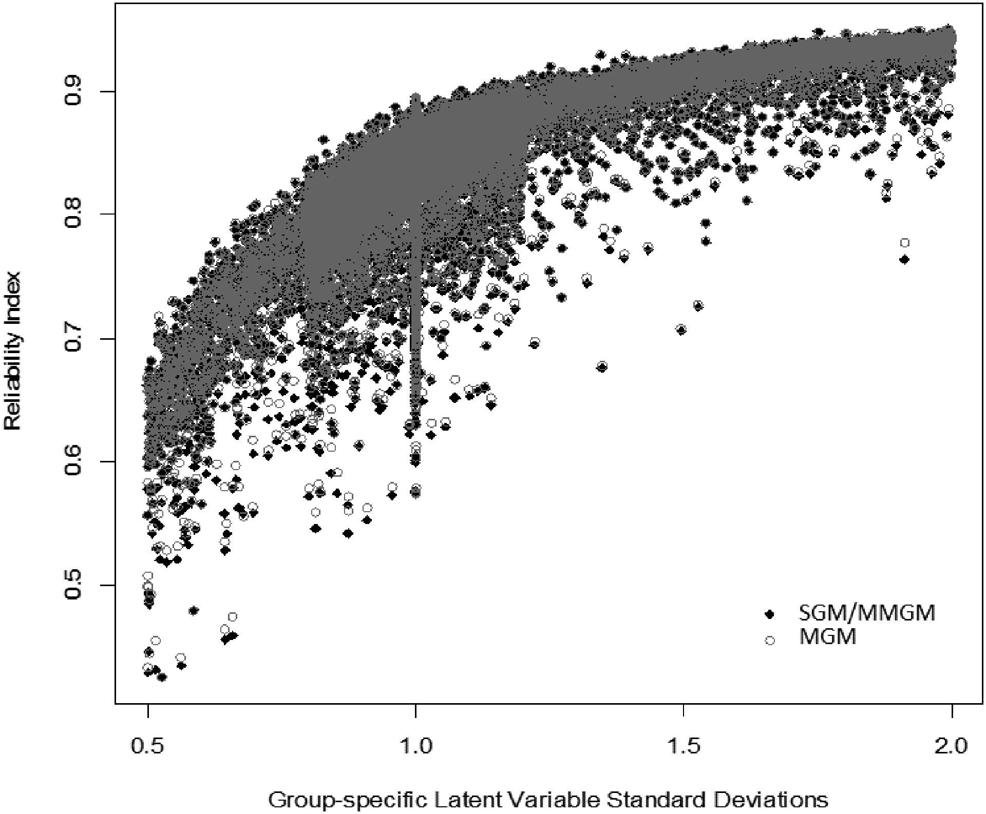
Group-specific true latent variable standard deviations plotted against group-specific reliability indices for the MGM approach versus the SGM and MMGM approaches

Note: SGM and MMGM approaches grouped because the values were nearly coincident.

Raw Differences between True and Estimated Latent Variable Scores

Next, we examined the raw differences between the true and estimated latent variable scores for each approach (i.e., true – estimated). The difference was calculated for each simulated individual in each group in each simulated dataset, and the mean and standard deviation of the difference scores was then calculated for each dataset. This process was repeated for the latent variable estimates obtained from each approach. A one way ANOVA with the mean raw difference as the outcome and approach as the factor indicated a non-significant difference between the three approaches to estimating latent variable scores, F(2, 67497) = 0.27, p = .77.

As was done with the reliability index, we examined the relations between the group-specific mean raw differences (averaged raw difference for each group in each dataset/approach combination) and the group-specific true latent variable means and standard deviations. There was no relation between the group-specific mean raw differences and latent variable standard deviations in any approach (r = −0.01, p = .40; r = 0.01, p = .43; r = 0.01, p = .43 for the MGM approach, the SGM approach, and the MMGM approach, respectively). However, there were associations between the population group means and the mean raw differences. For the SGM and MMGM approaches, there was a strong positive correlation between the group-specific mean of the raw differences and the group-specific true latent variable means (r = 0.93, p < .001). Thus, for large positive latent variable group-specific means, there were larger positive differences between true and estimated latent variable scores and for large negative latent variable means, there were larger negative differences between true and estimated latent variable scores. Therefore, the SGM and MMGM approaches tended to underestimate the magnitude of group differences (i.e., estimated scores were closer to 0 than the population scores). The reverse was true for the MGM approach, as the correlation between group-specific mean differences and group-specific latent variable means was strong and negative (r = −0.91, p < 0.001). Thus, the MGM approach tended to overestimate the magnitude of group differences (i.e., estimated scores were closer to their group-level means). These effects can be visualized in Figure 2, which is a plot of the group-specific mean raw differences as a function of group means. In sum, the SGM and MMGM approaches, which ignore group differences tended to underestimate group differences whereas the MGM approach, which recognizes group differences, tended to overestimate group differences and these effects were largest at the extremes (i.e., when large differences in the group means were observed).

Figure 2.

Group-specific true latent variable means plotted against group-specific mean raw differences for the MGM approach versus the SGM and MMGM approaches

Note: SGM and MMGM approaches grouped because the values were nearly coincident.

Root Mean Squared Difference (RMSD)

Finally, we assessed the RMSD for each approach. For each simulated individual, the difference between true and estimated latent variable scores was calculated and squared. The average squared differences were then calculated for each group and then square rooted. The mean RMSDs for the SGM and MMGM approaches were nearly identical, and these approaches produced slightly more accurate latent variable estimates than the MGM approach (t = −2.94, p < .01).

We investigated the relation between the RMSDs and latent variable means and standard deviations across the three approaches. Although significant at times, no practical relation was found between RMSDs and the latent variable means across the three approaches (r = −0.01, p = .23; r = −0.01, p < .05; and r = −0.01, p < .05, respectively). However, a positive association was found between RMSDs and the latent variable standard deviation indicating that groups with larger standard deviations had larger RMSDs, which can be seen in Figure 3, which is a plot of the true latent variable standard deviations against group-specific estimated RMSDs. Overall, groups with larger between-individual differences tended to show larger discrepancies between estimated and simulated latent variable scores. We then examined this association for the different approaches to estimating latent variable scores and found the association was stronger for the MGM approach compared to the SGM and MMGM approaches (t = 5.06, p < .001). The correlation between RMSD and group standard deviation with the MGM approach was 0.57 (p < .001), whereas this correlation was 0.41 for the SGM and MMGM approaches.

Figure 3.

Group-specific true latent variable standard deviations plotted against group-specific estimated RMSD for the MGM approach versus the SGM and MMGM approaches

Note: SGM and MMGM approaches grouped because the values were nearly coincident.

We further examined the differences in this association with an ANCOVA with group-specific RMSDs as the outcome variable and two dummy coded variables to compare the SGM and MMGM approaches to the MGM approach, the group standard deviation, and their products as the input variables to examine interactive effects. The interactions were significant, highlighting differences in the strength of the association between group standard deviation and RMSD. The interaction coefficients were identical, b = −0.082, suggesting that the relation between RMSD and group standard deviations was less strong for the SGM and MMGM approaches compared to the MGM approach. The estimated cross-over point (see Widaman, Helm, Castro-Schilo, Pluess, Stallings, & Belsky, 2012) for the interaction was 1.00 indicating that the SGM and MMGM approaches provided more accurate latent variable estimates for groups with large standard deviations, whereas the MGM approach provided more accurate estimates for groups with small standard deviations.

Discussion

Our interest lies in the accuracy of latent variable score estimates from multiple group item response data. Latent variable score estimates from a typically specified multiple group item response model lacked consistency between the individuals’ item response patterns and their latent variable score estimates. The lack of consistency in latent variable score estimates was illustrated using multisample item-level data on violence perpetration, and was due to mean differences in the level of violence across samples. The lack of consistency was concerning because, from a test score bias perspective, latent variable score estimates should be based on the participants’ responses as opposed to background variables. Given our concern for latent variable score estimates from the typically specified multiple group item response model (MGM approach), we examined the accuracy of latent variable score estimates from two alternative item response models. The first was a single group item response model (SGM approach) and the second was a multiple group model with latent variable distributions equated across groups (MMGM approach). The accuracy of latent variable score estimates across the three approaches was examined through Monte Carlo simulations.

The results of the Monte Carlo simulations suggested that the SGM and MMGM approaches led to nearly identical estimated latent variable scores and these two approaches performed equally well to the MGM approach, outperformed the MGM approach under certain circumstances, and underperformed the MGM approach in others. Specifically, in examining the relation between latent variable standard deviations and latent variable score estimate accuracy quantified by the RMSD, estimated latent variable scores from the SGM and MMGM approaches were more accurate than estimates obtained from the MGM approach when the group’s latent variable standard deviation was greater than one. The SGM and MMGM approaches performed worse when the group’s latent variable standard deviation was less than one.

We also found that the latent variable estimates from the SGM and MMGM approaches underestimated group mean differences, whereas the MGM approach overestimated group differences. These results can be attributed to the shrinkage of estimated latent variable scores to their prior distribution (Grice & Harris, 2010). That is, estimated latent variable scores tend to be closer to their mean. Thus, the standard deviation of estimated latent variable scores tended to be smaller than the estimated standard deviation of the latent variable.

The results of the simulation suggest minor differences in the overall accuracy of latent variable score estimates from the three approaches. However, the one-to-one mapping of response patterns with factor score estimates is an important benefit of the SGM and MMGM approaches, especially when some response patterns are not particularly informative. These approaches also ensure that a participant’s latent variable score estimate is solely based on the items asked and the participant’s responses, and not based on the responses of other associated participants (e.g., members of the same gender or study). For these reasons, we feel that it is important for the prior distribution to be the same when estimating latent variable scores.

Ignoring group information when estimating latent variable scores is common in item response modeling. That is, the estimation of the latent variable model parameters has often been separated from the estimation of the latent variable scores. For example, in the Multilog program (Thissen, Chen, & Bock, 2003), calibration of item parameters took place in the first run, and the scoring of the individuals (latent variable score estimation) took place in a second run. In this second run, the model’s parameters were treated as fixed. And if latent variable estimates were needed for a new sample, their item response data could be scored (as in the second run above) with all of the model’s parameters (discriminations, locations, latent variable mean and variance) fixed to their previously estimated values. This approach ensured that there was a one-to-one mapping of latent variable score estimates and response patterns, which we feel is integral to any scoring procedure.

Given Multilog’s approach, it may be best to separate the estimation of model parameters from the estimation of latent variable scores. For example, the standard multiple group item response model can be specified to estimate model parameters. Once estimated, a single group model can be specified with item parameters fixed at their previously estimated values with the mean and variance of the latent variable set to 0 and 1, respectively. This two-step approach would ensure that item parameters are not biased when estimating latent variable scores, which is a possibility in the SGM and MMGM approaches.

Prior Distribution of Latent Variable Score Estimates

The reason for the inconsistencies between response patterns and latent variable score estimates across samples in the MGM approach was due to differences in the prior distribution of the latent variable score estimates across samples. The prior distribution came from the sample’s estimated mean and variance of the latent variable. Thus, the prior came from information obtained from the sample (i.e., group in the multiple group model) the participant belonged. Recently, researchers have recommended using covariate-informed latent variable estimates (Curran, Cole, Bauer, Hussong, & Gottfredson, 2016; Curran, Cole, Bauer, Rothenberg, & Hussong, 2018), which allows covariates to inform the prior distribution of the latent variable score estimates. Thus, covariate-informed latent variable estimates will lack consistency – there will not be a one-to-one mapping between response patterns and latent variable score estimates.

While the covariate-informed latent variable score estimation approach can lead to more accurate associations when the effects of covariates are properly specified, we caution against their use for three reasons. First, when the scoring of a construct is partially based on covariate information, there is an assumption that the covariate information is properly specified. This assumption is quite strong because we typically consider only linear and additive effects (i.e., no nonlinear associations or interactions). Second, when the response pattern is not very informative, the prior distribution dominates the estimation of latent variable score. This was the case with the illustrative data because the most common response pattern was one where none of the items were endorsed and we observed wide ranging latent variable score estimates for individuals with this response pattern. In these cases, the latent variable score estimate tells us more about who the person is rather than their item responses if covariate-informed latent variable estimates are used. Third, when covariates inform latent variable estimation, latent variable scores can be estimated for participants who have not responded to any of the indicator items. In these situations, the estimated latent variable score is solely based on the prior distribution.

While our focus is on prior distributions when estimating latent variable scores, researchers have highlighted similar issues in latent variable models, more generally. That is, there are latent variable models where determinants or consequents of the latent variable affect the measurement of the latent variable itself. Levy (2017) highlights this issue where the factor loadings differ when an outcome of the latent variable was included in the model. That is, when the latent variable was specified with its indicators, the factor loadings were all strong suggesting the latent variable was well defined. The model was then extended to include an outcome. When this model was estimated, the factor loadings were noticeably smaller and varied in strength compared to when the factor model was previously estimated. Levy proposed a multistep procedure to distinguish indicators and outcomes in latent variable models to resolve this issue.

A second example comes from finite mixture models, where the latent class variable can be strongly affected by predictors of class membership. That is, including predictors of class membership can make the latent class variable more representative of the predictors than the indicators of class membership (see Stegmann & Grimm, 2017). This issue in finite mixture modeling led researchers to propose multistep procedures to eliminate the effect of predictors on the formation of the latent class variable (Asparouhov & Muthén, 2014). Thus, these two examples highlight how researchers have tried to eliminate or reduce the influence of covariates in the measurement of a latent variable.

Factor Score Regression

The research presented here on the accuracy of latent variable score estimates is also related to factor score regression (FSR; Skrondal & Laake, 2001), which is a stepwise estimation procedure for structural equation models (SEM) where researchers use estimated factor scores as observed data in subsequent analyses. The steps of FSR include: (1) estimate parameters in measurement model, (2) estimate factor scores in EFA or CFA using estimated parameters, (3) perform regression analysis, path analysis, or factor analysis, where variables in model are the estimated factor scores. Although using factor scores as observed variables remedy potential issues with SEM’s simultaneous estimation, the factor scores are linear combinations of variables that include error and can produce biased estimates in subsequent analyses (Hoshino & Bentler, 2011). Therefore, various methods of FSR have been developed to account for this bias (e.g., Croon, 2002; Skrondal & Laake, 2001). The focus of this work is on the estimation of the latent variable regression parameters and bias that is introduced because of the factor score regression, as opposed to the accuracy of latent variable scores. We note that Skrondal and Laake (2001) highlight the importance of estimating the latent variable scores separately for each latent variable, which separates the latent variable score estimation from its prediction.

Limitations

The simulations focused on latent variable estimates from fitting different item response models to multisample item level data. As such, we varied the latent variable’s means and standard deviations across groups to evaluate their impact on the accuracy of estimated latent variable scores from each of the three approaches. We did not, however, vary the number of items, the number of response categories per item, or examine the impact of incomplete data. We expect the accuracy of the latent variable estimates to improve with more items and with items with more response categories. We also expect the observed differences between the modeling approaches will be minimized with more items and items with more response categories because there is likely to be greater information in the response patterns.

Although we varied the magnitude of the discrimination and location parameters in the population, we did not report on their impact because their effects were in the expected directions. That is, replicates with greater discrimination parameters tended to have more accurate estimates based on the reliability index, raw differences, and RMSDs. Location parameters were not significantly associated with the accuracy indices. From these results, we simply note the importance of having high discriminating items that are well targeted to the population of interest.

In our simulations, item parameters were invariant across the multiple populations from which the data were sampled. In empirical studies, there is usually some lack of measurement invariance whether it is observable or not. We expect the results would be weaker (i.e., larger differences between estimated and actual latent variable scores) when strong measurement invariance does not hold in the population.

Finally, we only examined EAP latent variable score estimates and did not examine Modal A Posteriori (MAP) estimates in our simulation. EAP and MAP estimates tend to be highly related and in our empirical data, MAP estimates showed very similar patterns to the EAP estimates. Thus, we expect our results to generalize to MAP estimates.

Concluding Remarks

The notable results lie in the extent to which the prior distribution of the estimated latent variable scores can affect the estimates of the latent variable score for individuals with less informative response patterns, and how ignoring group differences when estimating latent variable scores can produce estimated latent variable scores that are equally accurate. Ignoring group differences has the added benefit of separating the estimation of the latent variable scores from their prediction and leads to a one-to-one mapping between response patterns and estimated latent variable scores. Thus, we recommend ignoring group differences when estimating latent variable scores. However, when using this approach, we encourage researchers to examine the measurement parameters when using the SGM and MMGM approaches to determine if they differ significantly from when the proper multiple group model is specified. If the measurement parameters are noticeably different, then the measurement parameters should be fixed to their estimates from the properly specified multiple group model and the latent variable mean and variance should be fixed to the same values (e.g., 0 and 1, respectively) in all groups.

Our interest lies in the estimates of latent variables because IDA is dependent on such estimates due to the size of the studies being integrated and the complexity of the subsequent analyses (i.e., IDA studies are often longitudinal). The issue discussed here is not relevant when remaining in the latent variable framework; however, in IDA, where latent variable score estimates are needed, accurately estimated latent variable scores is of utmost importance.

The present work also highlights potential issues when utilizing item parameters from one study and applying them to another study to estimate latent variable scores to aid comparability. Unless the latent variable distributions are equal in the two studies, the estimated latent variable scores for individuals from different samples can differ even though the same response patterns are observed. However, fixing the distribution of the latent variables to be equal in the two studies will result in consistent latent variable estimates that are just as accurate.

Finally, we note that this issue is likely to be exacerbated with repeated measures data. With repeated measures multisample data, the properly specified item response model is a multiple group multilevel model (Kamata, 2001; Muthén & Asparouhov, 2002) where each individual has his or her own distribution. Furthermore, fitting a change trajectory within the multiple group multilevel model further impacts latent variable estimates (see McArdle et al., 2009). Future research should investigate the influence of model specification on the accuracy and consistency of estimated latent variable scores from multiple group longitudinal data.

References

- Adams RN, Mosher CE, Blair CK, Snyder DC, Sloane R, & Demark-Wahnefried W (2015). Cancer survivors’ uptake and adherence in diet and exercise intervention trials: an integrative data analysis. Cancer, 121, 77–83. [DOI] [PMC free article] [PubMed] [Google Scholar]
- Asparouhov T & Muthén B (2014). Auxiliary variables in mixture modeling: Three-step approaches using Mplus. Structural Equation Modeling: A Multidisciplinary Journal, 21, 329–341. [Google Scholar]
- Cai L (2013). flexMIRT® version 2: Flexible multilevel multidimensional item analysis and test scoring [Computer software]. Chapel Hill, NC: Vector Psychometric Group. [Google Scholar]
- Croon M (2002). Using predicted latent scores in general latent structure models. In Marcoulides G & Moustaki I (Eds.), Latent variable and latent structure modeling (pp. 195–223). Mahwah, NJ: Lawrence Erlbaum. [Google Scholar]
- Curran PJ, Cole V, Bauer DJ, Hussong AM, & Gottfredson N (2016). Improving factor score estimation through the use of observed background characteristics. Structural Equation Modeling: A Multidisciplinary Journal, 23, 827–844. [DOI] [PMC free article] [PubMed] [Google Scholar]
- Curran PJ, Cole VT, Bauer DJ, Rothenberg WA, & Hussong AM (2018). Recovering predictor–criterion relations using covariate-informed factor score estimates. Structural Equation Modeling: A Multidisciplinary Journal, 25, 860–875. [DOI] [PMC free article] [PubMed] [Google Scholar]
- Curran PJ, & Hussong AM (2009). Integrative data analysis: The simultaneous analysis of multiple data sets. Psychological Methods, 14, 81–100. [DOI] [PMC free article] [PubMed] [Google Scholar]
- Curran PJ, Hussong AM, Cai L, Huang W, Chassin L, Sher KJ, & Zucker RA (2008). Pooling data from multiple prospective studies: The role of item response theory in integrative analysis. Developmental Psychology, 44, 365–380. [DOI] [PMC free article] [PubMed] [Google Scholar]
- Desmarais SL, Van Dorn RA, Johnson KL, Grimm KJ, Douglas KS, & Swartz MS (2014). Community violence perpetration and victimization among adults with mental illnesses. American journal of public health, 104, 2342–2349. [DOI] [PMC free article] [PubMed] [Google Scholar]
- Duncan GJ, Dowsett CJ, Claessens A, Magnuson K, Huston AC, Klebanov P, Pagani LS, Feinstein L, Engel M, Brooks-Gunn J, Sexton H, Duckworth K, & Japel C (2007). School readiness and later achievement. Developmental Psychology, 43, 1428–1446. [DOI] [PubMed] [Google Scholar]
- Glass GV (1976). Primary, secondary, and meta-analysis. Educational Researcher, 5, 3–8. [Google Scholar]
- Grice JW, & Harris RJ (2010). A comparison of regression and loading weights for the computation of factor scores. Multivariate Behavioral Research, 33, 221–247. [DOI] [PubMed] [Google Scholar]
- Hallquist M, & Wiley J (2013). MplusAutomation: Automating Mplus Model Estimation and Interpretation. R package version 0.6–1. http://CRAN.Rproject.org/package=MplusAutomation [Google Scholar]
- Hofer SM, & Piccinin AM (2009). Integrative data analysis through coordination of measurement and analysis protocol across independent longitudinal studies. Psychological Methods, 14, 150–164. [DOI] [PMC free article] [PubMed] [Google Scholar]
- Hofer SM, & Piccinin AM (2010). Toward an integrative science of lifespan development and aging. Journals of Gerontology: Psychological Sciences, 65B, 269–278. [DOI] [PMC free article] [PubMed] [Google Scholar]
- Horwood LJ, Fergusson DM, Coffey C, Patton GC, Tait R, Smart D, Letcher P, Silins E, & Hutchinson DM (2012). Cannabis and depression: an integrative data analysis of four Australasian cohorts. Drug and Alcohol Dependence, 126, 369–378. [DOI] [PubMed] [Google Scholar]
- Hoshino T, & Bentler PM (2011). Bias in factor score regression and a simple solution. UCLA Statistics Preprint #621. http://preprints.stat.ucla.edu [Google Scholar]
- Kamata A (2001). Item analysis by the hierarchical generalized linear model. Journal of Educational Measurement, 38, 79–93. [Google Scholar]
- Kay SR, Fiszbein A, & Opler LA (1987). The positive and negative syndrome scale (PANSS) for schizophrenia. Schizophrenia Bulletin, 13, 261–276. [DOI] [PubMed] [Google Scholar]
- Levy R (2017). Distinguishing outcomes from indicators via Bayesian modeling. Psychological Methods, 22, 632–648. [DOI] [PubMed] [Google Scholar]
- Lieberman JA, Stroup TS, Mcevoy JP, Swartz MS, Rosenheck RA, Perkins DO, et al. (2005). Effectiveness of antipsychotic drugs in patients with chronic schizophrenia. New England Journal of Medicine, 353, 1209–1223. [DOI] [PubMed] [Google Scholar]
- Luningham JM, McArtor DB, Hendriks A, van Beijsterveldt CE, Lichtenstein P, Lundström S, Larsson H, Bartels M, Boomsma DI, & Lubke G (2019). Data integration methods for phenotype harmonization in multi-cohort genome-wide association studies with behavioral outcomes. Frontiers in Genetics, 10, 1227. [DOI] [PMC free article] [PubMed] [Google Scholar]
- McArdle JJ, Grimm KJ, Hamagami F, Bowles R, & Meredith W (2009). Modeling life-span growth curves of cognition using longitudinal data with multiple samples and changing scales of measurement. Psychological Methods, 14, 126–149. [DOI] [PMC free article] [PubMed] [Google Scholar]
- McArdle JJ, Hamagami F, Meredith W, & Bradway KP (2000). Modeling the dynamic hypotheses of Gf-Gc theory using longitudinal life-span data. Learning and Individual Differences, 12, 53–79. [Google Scholar]
- McArdle JJ, Prescott CA, Hamagami F, & Horn JL (1998). A contemporary method for developmental-genetic analyses of age changes in intellectual abilities. Developmental Neuropsychology, 14, 69–114. [Google Scholar]
- McDonald RP (1999). Test theory: A unified treatment. New Jersey: Lawrence Erlbaum Associates, Inc. [Google Scholar]
- McGrath KV, Leighton EA, Ene M, DiStefano C, & Monrad DM (in press). Using integrative data analysis to investigate school climate across multiple informants. Educational and Psychological Measurement. [DOI] [PMC free article] [PubMed] [Google Scholar]
- Meade AW, & Lautenschlager GJ (2004). A comparison of item response theory and confirmatory factor analytic methodologies for establishing measurement equivalence/invariance. Organizational Research Methods, 7, 361–388. [Google Scholar]
- Meredith W (1993). Measurement invariance, factor analysis, and factorial invariance. Psychometrika, 58, 525–543. [Google Scholar]
- Monahan J, Bonnie RJ, Appelbaum PS, Hyde PS, Steadman HJ, Swartz MS (2005). Mandated community treatment: Beyond outpatient commitment. Psychiatric Services, 52, 1198–1205. [DOI] [PubMed] [Google Scholar]
- Muthén BO, & Asparouhov T (2002). Latent variable analysis with categorical outcomes: Multiple group and growth modeling in Mplus. Mplus Web Notes: No. 4 [Google Scholar]
- Muthén LK, & Muthén BO (1998–2011). Mplus User’s Guide. Sixth Edition. Los Angeles, CA: Muthén & Muthén. [Google Scholar]
- Overall JE, & Gorham DR (1962). The brief psychiatric rating scale. Psychological Reports 10, 790–812. [Google Scholar]
- R Core Team (2013). R: A language and environment for statistical computing. R Foundation for Statistical Computing, Vienna, Austria. URL http://www.R-project.org/. [Google Scholar]
- Reise SP, Widaman KF, & Pugh RH (1993). Confirmatory factor analysis and item response theory: Two approaches for exploring measurement invariance. Psychological Bulletin, 114, 552–566. [DOI] [PubMed] [Google Scholar]
- Skrondal A, & Laake P (2001). Regression among factor scores. Psychometrika, 66, 563–575. [Google Scholar]
- Smith ML, & Glass GV (1977). Meta-analysis of psychotherapy outcome studies. American Psychologist, 32, 752–760. [DOI] [PubMed] [Google Scholar]
- Steadman HJ, Mulvey EP, Monahan J, Robbins PC, Appelbaum PS, Grisso T, et al. (1998). Violence by people discharged from acute psychiatric inpatient facilities and by others in the same neighborhoods. Archives of General Psychiatry, 55, 393–401. [DOI] [PubMed] [Google Scholar]
- Stegmann G, & Grimm KJ (2018). A new perspective on the effects of covariates in mixture models. Structural Equation Modeling: A Multidisciplinary Journal, 25, 167–178. [Google Scholar]
- Swanson JW, Swartz MS, Elbogen EB (2004). Effectiveness of atypical antipsychotic medications in reducing violent behavior among persons with schizophrenia in community-based treatment. Schizophrenia Bulletin, 30, 3–20. [DOI] [PubMed] [Google Scholar]
- Swanson JW, Swartz MS, Elbogen EB, Van Dorn RA, Ferron J, Wagner HR, et al. (2006). Facilitated psychiatric advance directives: A randomized trial of an intervention to foster advance treatment planning among persons with severe mental illness. American Journal of Psychiatry, 163, 1943–1951. [DOI] [PMC free article] [PubMed] [Google Scholar]
- Terman LM (1916). The measurement of intelligence. An explanation of and a complete guide for the use of the Stanford revision and extension of The Binet-Simon Intelligence Scale Cambridge, MA: Riverside Press. [Google Scholar]
- Terman LM, & Merrill MA (1937). Measuring intelligence: A guide to the administration of the new revised Stanford-Binet test of intelligence. Oxford, England: Houghton Mifflin. [Google Scholar]
- Terman LM, & Merrill MA (1960). Stanford-Binet Intelligence Scale: Manual for the Third Revision Form L-M. Boston, MA: Houghton Mifflin. [Google Scholar]
- Thissen D, Chen W-H, & Bock RD (2003). MULTILOG 7 for Windows: Multiple category item analysis and test scoring using item response theory [Computer software]. Skokie, IL: Scientific Software International, Inc. [Google Scholar]
- Wechsler D (1939). The measurement of adult intelligence. Baltimore: Williams & Wilkins [Google Scholar]
- Wechsler D (1955). Manual for the Wechsler Adult Intelligence Scale. New York: The Psychological Corporation. [Google Scholar]
- Wechsler D(1981). The Wechsler Adult Intelligence Scale – Revised. New York: The Psychological Corporation. [Google Scholar]
- Widaman KF, Helm J, Castro-Schilo L, Pluess M, Stallings MC, & Belsky J (2012). Distinguishing ordinal and disordinal interactions. Psychological Methods, 17, 615–622. [DOI] [PMC free article] [PubMed] [Google Scholar]
- Widaman KF, & Reise SP (1997). Exploring the measurement invariance of psychological instruments; Applications in the substance use domain. In Bryant KJ, Windle M, & West SG (Eds.), The science of prevention: Methodological advances from alcohol and substance use research (pp. 281–324). Washington DC: American Psychological Association. [Google Scholar]