An Epidemiological Neural Network Exploiting Dynamic Graph Structured Data Applied to the COVID-19 Outbreak

Abstract

With the recent COVID-19 outbreak, we have assisted to the development of new epidemic models or the application of existing methodologies to predict the virus spread and to analyze how the different lock-down strategies can effectively influence the epidemic diffusion. In this paper, we propose a novel machine learning based framework able to estimate the parameters of any epidemiological model, such as contact rates and recovery rates, based on static and dynamic features of places. In particular, we model mobility data through a graph series whose spatial and temporal features are investigated by combining Graph Convolutional Neural Networks (GCNs) and Long short-term memories (LSTMs) in order to infer the parameters of SIR and SIRD models. We evaluate the proposed approach using data related to the COVID-19 dynamics in Italy and we compare the forecasts of the trained model with available data about the epidemic spread.

1. Introduction

The first atypical case of pneumonia from which the SARS-CoV-24 virus began to spread was diagnosed in December 2019 in Wuhan, Hubei province of China [1], [2], [3]. The virus belongs to the same virus family of the Severe Acute Respiratory Syndrome (SARS) that outbroke in South China in 2002-2003 [4]. Despite the radical measures taken by the Chinese authorities to contain the outbreak [5], it managed to spread across the whole world, thus being declared as a pandemy by the World Health Organization.¹

The history of pandemic evolution in Italy, one of the most affected countries outside of Asia, can be summarized as follows:²

• 1)January, 30 - suspension of flights from and to China
• 2)January, 31 - two Chinese tourists are positive to the coronavirus
• 3)February, 21 - in Codogno (LO), the first infected Italian is found out, and in a few hours a huge number of other infected individuals follows
• 4)February, 23 - some Municipalities in Lombardy and Veneto are considered to be “red zones” with prohibitions of accesses and departures within the area
• 5)March, 4-7 - schools are closed and the national lock-down begins
• 6)April, 5 - number of infected individuals starts to decrease
• 7)May - the pandemic epicentre moves to the American continent and in Italy the lock-down “second phase” starts, trying to trigger the economic recovery.

Just to report some numbers of Sars-Cov-24 pandemic, at time of the report (30th May, 2020), the total number of detected cases in Italy were 240.436, of which 16.496 were currently infected (1.120 hospitalized, 96 admitted to Intensive Care Units, 15.280 isolated at home), 189.196 were healed and discharged, and 34.744 died.

During the pandemic, scientists of all the world have tried to apply more or less complex models of different nature in order to predict the real virus spread, and to analyze as possible lock-down measures can influence the epidemic diffusion.

As well-known, mathematical models are usually the most used to understand how viruses spread across individuals [6], [7], [8], [9], including the SIR model [10], which takes into account three mutually exclusive stages of infection: Susceptible (S), Infected (I) and Recovered (R). SIR model is widely diffused thanks to its clarity and straightforwardness, but the measures which humans take to prevent the disease spreading make the understanding of the disease transmission dynamics a major challenge [11]. According to [12], approaches which incorporate preventive behaviors in mathematical models fall into two general categories: the first incorporating the effects of preventive behaviors into disease model parameters (e.g., [13], [14], [15]), and the second introducing new dynamic states with the aim to distinguish who have adopted a preventive behavior from those who have not (e.g., [16], [17], [18]).

During the last decade, Machine Learning (ML) algorithms have then offered alternative solutions to the virus spread prediction [19], [20], [21].

One of the first studies using ML techniques on coronavirus-related data [22] identified the global spread of the disease through commercial airlines. In the various papers, ML is directly used to predict epidemic diffusion on the basis of past information, or can be properly exploited to infer the parameters of epidemiological models, using as an example further information (e.g., user mobility).

In this paper, in according to the second class of approaches, we propose a ML-based framework to estimate parameters of a generic epidemiological model fitting the observed trends on the basis of users’ movements during lock-down. In particular, our model integrates mobility rates between regions modeling data through a graph data structure whose spatial and temporal features are investigated by combining Graph Convolutional Neural Networks (GCNs) and Long short-term memories (LSTMs). To the best of our knowledge, this is the first time that spatio-temporal data mining techniques have been employed to predict the spread of an epidemic.

Furthermore, our model can be easily applied to different kinds of spatial entities (e.g., regions, provinces, municipalities, etc.) for unveiling different virus trends among the different places.

We evaluate the proposed approach with a case study which analyses the COVID-19 outbreak in Italy from February 24th to May 5th and compares the forecasts of the trained model with real data on the epidemic.

The paper is organized as in the following. Section 2 outlines the Related Works concerning the most diffused predictive models for estimating epidemic spread. Section 3 describes the Theoretical Background at the basis of our approach. Section 4 details the proposed Methodology used to estimate epidemic model parameters. Section 5 reports the Case Study with some experimental results. Finally, Sections 6 presents Conclusions and Future Work.

2. Related Work

In the last decades several epidemiological models, describing influence diffusion as a disease spread among biological populations by a given infection rate, have been widely studied in literature. One of the mostly used models is the Susceptible-Infected-Recovered (SIR) model, in which when an individual recovers from the disease he acquires a permanent immunity or is removed. In this models the infection process involves a contact among two or more users while the others process occur spontaneously after a certain time.

The COVID-19 outbreak pushed for the definition of new models and approaches for the analysis of its diffusion. Situational information about COVID-19 based on information extracted from Sina Weibo has been proposed in [23] where a predictive task and a linear model whose weights are the main factors determining the propagation of situational information. In turn, [20] uses LSTMs to predict number of new infections over time using the 2003 SARS epidemic statistics incorporating the COVID-19 epidemiological parameters (e.g., probability of transmission, incubation rate, probability of recovery and death).

However, the majority of the proposed models can be seen as extensions of the SIR model. Numerical analyses based on SIR model have been discussed in [24], [25] analyzing COVID-19 national statistics: the former defining a time-dependent SIR model for investigating spread diffusion based on Independent Cascade model and for predicting the national peak and end of epidemic, the latter analyzing lock-down effects on the basis of different variants of the Susceptible-Exposed-Infected-Recovered (SEIR) model. In [21] the spread of the COVID-19 based on mobility data has been predicted by using SIRNet, an hybrid machine learning model coupling with epidemiological models. [26] presents an early prediction of the epidemic disease based on a simplified SIR model, in which the population is governed by a system of three nonlinear ordinary equations with the infection rate $\beta$ and the removal rate $\gamma$ as parameters. In [27] the authors perform Bayesian inference to find the central epidemiological parameters of a SIR model. They consider a time-dependent infection rate via potential change points reflecting changes in the spreading rate driven by governmental interventions. A time-dependent SIR model where both the transmission rate $\beta$ and the recovery rate $\gamma$ are functions of the time $t$ has been proposed in [24]. They predict the time-dependent parameters using FIR filters and ridge regression: essentially, $\widehat{\beta }\left(t\right)$ is a linear combination of the same parameter computed in the previous time steps.

Considering the Italian situation, Giordano et al. [28] extend the classical SIR model considering the diagnosed/non-diagnosed cases, the severity of the symptoms and dividing the recovered patients from dead ones. More in detail, they recast the differential equations systems in a feedback structure and define the conditions that the parameters should respect in order to have asymptotic stability. In other words, they simulate a dynamic system with five states and three outputs whose evolution depends on 16 parameters, which are varied empirically considering the different levels of social-distancing countermeasures taken by Italian government.

Nevertheless, the cited approaches suffer from different drawbacks. Although SIRNET [21] shows the relevance of mobility data in the transmission of the epidemic, it does not consider the mobility between nodes (or places) fitting its analysis on a single region. In turn, [27] and [26], [28] are only based on temporal analysis and diffusion process respectively. Moreover, they require the manual optimization of their hyper-parameters which might become too difficult when the dynamics of the evolution tangle or the number of parameters increases.

In this paper we aimed to overcome these limitations by combining Graph Neural Networks (GNN) with Recurrent Neural Network (RNN) for modeling the spatial and temporal components of the graph sequence. Different approaches following this idea have been proposed for several applications: for example, [29] investigates some architectures based on RNNs and CNNs aiming to learn spatio-temporal structures from graph-structured and time-varying data, applying them to video prediction and natural language modeling, while [30] combines LSTMs and GCNs to exploit structural and temporal information of data to solve supervised and semi-supervised classification tasks. [31] proposes a recurrent architecture which allows GCN parameters to evolve based on the evolution of the inputs and the topological structure of the graph.

The original contributions of this work is twofold: i) the epidemic diffusion has been modelled as a spatio-temporal problem represented with a time-variant graph, whose nodes and edges represent respectively places where the infections occur, and movements between places; ii) graph convolutional networks (GCNs) and sequential deep learning techniques (e.g., GRUs, LSTMs) have been employed to tune the time-varying parameters of an epidemiological model (e.g., contact rates, recovery rates).

As a result, the final model is able to accurately fit real epidemic trends. In contrast to standard approaches which model the disease diffusion in a place as a whole [21], our framework can jointly model the diffusion in different regions and provinces for unveiling different virus trends among different places and takes into account the mobility data between them, which is useful to understand how epidemic trends of near places affect each others.

Finally, the proposed architecture has been evaluated with a case study on Italian infections at different granularity levels (regions, provinces), differently from the other approaches [24], [25] which only focus on national statistics.

3. Theoretical Background

In this section we introduce some basic notions on which our approach relies on. In particular, we first describe two main deep learning techniques (Graph Convolutional Networks and Long-short Term Memory), representing the fundamentals of the proposed model, and successively we focused on the main epidemiological models.

3.1. Graph Convolutional Networks

Graph machine learning has the primary challenge of finding a way to represent graph structure so that it can be easily exploited by machine learning models; in particular, the Graph Convolutional Networks (GCN) are the generalization of the standard Convolutional Neural Networks, used to extract low-level features from image data, and are based on the idea that not only does the best nodes’ representation depend by their own characteristics, but also by their neighbourhood description and topology.

Formally, let $\mathcal{G}=(\mathcal{V},\mathcal{E})$ be a generic graph, $\mathcal{V},\mathcal{E}$ being the nodes and edges sets respectively, and consider its adjacency matrix $A$; then each layer $H^{\left(l\right)}$ is defined recursively as follows [32]:

$$H^{(l+1)}=f(H^{\left(l\right)},A)=\sigma ({\widehat{D}}^{-1/2}·\widehat{A}·{\widehat{D}}^{-1/2}·H^{\left(l\right)}·W^{\left(l\right)}),\left(\left(1\right)\right)$$

$\sigma$ being an activation function, $\widehat{A}=A+I$ (I is the identity matrix), $\widehat{D}$ being the nodes diagonal node degree matrix of $\widehat{A}$, $W^{\left(l\right)}$ being the (learnable) weight matrix for the l-th layer.

Many variants of this model have been proposed in literature to deal with directed and/or weighted and/or dynamic graphs. Anyway, graph neural networks have proven their effectiveness in a wide range of application domains performing nodes, edges and graph classification: for example, in computer vision they are extensively used for scene graph generation and for classifying and segmenting points clouds [33], [34]; in NLP they can perform text classification and sentences generation [32], [35]; in chemistry they are usually employed to learn molecular fingerprints and predict molecular properties [36], [37].

3.2. Recurrent Neural Networks

The learning problem analyzed throughout this work involves the processing of sequences of data, i.e., the dynamically changing graph of places with their movement flows and their infection information. Recurrent Neural Networks (RNNs) have been designed to achieve this goal through connections that form directed cycles. They have been particularly successful for many tasks involving time-series data, such as handwriting [38] and speech recognition [39]. These networks apply linear matrix operations to the current observation and the hidden units resulting from the previous step, and the resulting linear terms are arguments of activation functions act():

$$\begin{array}{c}\hfill {\mathbf{h}}_t=act({\mathbf{W}}_{\mathbf{h}}{x}_t+{\mathbf{U}}_h{\mathbf{h}}_{t-1}+{\mathbf{b}}_h)\\ \hfill {\mathbf{o}}_t=act({\mathbf{W}}_0{\mathbf{h}}_t+{\mathbf{b}}_0).\left(\left(2\right)\right)\end{array}$$

A recurrent neural network uses the same matrix ${\mathbf{U}}_h$ at each time step, and the gradient can vary easily either explode or vanish over many steps [40]. Long Short-Term Memories (LSTMs) [41] are an evolution of RNNs specifically created to address the vanishing gradient problem. They are designed to retain information without modification for long periods of time in ”memory cells” controlled by input and output gates. For each time step, through element-wise product and sums between units, input gates are used to determined whether a potential input (computed as a linear combination of the current input value and the previous hidden unit vector) is sufficiently important to be placed into the memory unit; forget gates [42] allow the content of memory units to be erased and output gates determine whether the content of the memory units transformed by activation functions should be placed in the hidden unit of the time step $t$.

A wide number of other recurrent network architectures have been proposed, among which it is worth mentioning Gated Recurrent Units (GRUs)[43], which simplify LSTMs and can provide, for some problems, comparable performance with LSTMs but with a lower memory requirement.

3.3. Epidemic Modeling

Infectious diseases modelling aims to understand whether or how a virus can spread among a population. Compartmental models are the most used mathematical tool to accomplish the task, they divide the population into compartments and define how people may progress between them. In most cases, these models can be described through ordinary differential equations and rely on the estimation of various epidemiological parameters (e.g., the contact and recovery rates) representing the interaction between compartments.

The simplest compartmental models is the SIR model where the population is divided into three groups: the susceptible (S) represents people not yet infected, the infected (I) groups individuals that contract the disease and can contribute to its spread, and the recovered (R) compartment clusters individuals who are not infected anymore, including death ones. In particular, susceptible people may become infectious depending on the contact rate $\beta$ they have with other ill people, as well as infectious ones may heal (or die) after the removal time $T_r=1/\gamma$, $\gamma$ being the recovery rate. Formally:

$$\begin{array}{cc}\hfill S_{t+1}& =S_t-\beta \frac{SI}{N}\hfill \\ \hfill I_{t+1}& =I_t+\beta \frac{SI}{N}-\gamma I\hfill \\ \hfill R_{t+1}& =R_t+\gamma I,\left(\left(3\right)\right)\hfill \end{array}$$

N being the number of people in the population.

The common parameter used to describe the strength of the epidemic is the basic reproduction number $R_0=\beta /\gamma$, which represents the expected number of cases directly generated by one case in a population where all individuals are susceptible to infection. Specifically, $R_0>1$ means the disease will spread among the population, otherwise it is controlled and the number of cases will start decreasing.

A slight complication of the SIR model should be studied in order to model the dynamic of the dead people: the compartment of deaths (D) needs to be introduced and the death rate $\mu$ should control the transition between the infected compartment and the new one:

$$\begin{array}{cc}\hfill S_{t+1}& =S_t-\beta \frac{SI}{N}\hfill \\ \hfill I_{t+1}& =I_t+\beta \frac{SI}{N}-\gamma I-\mu I\hfill \\ \hfill R_{t+1}& =R_t+\gamma I\hfill \\ \hfill D_{t+1}& =D_t+\mu I.\left(\left(4\right)\right)\hfill \end{array}$$

All parameters are usually estimated considering the characteristic of the disease and optimized to fit at best the observed data. Forecast predictions are usually accomplished making hypotheses of how external factors (e.g., governmental countermeasures, vaccine distribution) affect the above-mentioned parameters.

4. Methodology

The COVID-19 pandemic has affected the whole world, in each place differently than others. The unpredictability of the infection spread is due to the complex causality relationships between features characterizing the contact rate between individuals and the increase of infections. Not only is the infection spread of a place attributable to its own features (e.g., number of inhabitants, population density, number of open shops) but it can also be imputed to the number of movements from other places. More importantly, an increase or decrease of movements can produce a change in the epidemic trends after an unclear or undefined period of time.

Our goal is to jointly exploit graph structured data and temporal information through the use of a neural network model in order to infer the dynamically-changing values of a standard epidemiological model (e.g., SIR, SEIR) parameters and thus study the effects of restriction measures imposed by local authorities on the virus spread behavior.

4.1. Data Model

From our viewpoint, the epidemic spread can be modeled by means of a dynamic graph in which nodes represent places (e.g., districts, municipalities, cities, states, regions, countries), and edges are the spread links of the epidemic, resulting from movements of infected individuals. Snapshots of the graph at different moments of time allow to depict the infection dynamics.

Throughout this work, we will refer to the following notation:

• •${\left({\mathcal{G}}_i\right)}_{i\in {\mathbb{Z}}_T}$, with ${\mathbb{Z}}_T=\{1,2,...,T\}$ is a finite sequence of directed weighted graphs ${\mathcal{G}}_i=(P_i,E_i,w_i)$, with $P_i=P\forall i\in {\mathbb{Z}}_T$, i.e., all the graphs in the sequence share the same nodes.
• •$x_i^k\in {\mathbb{R}}^d$ denotes the feature vector of the place $p^k\in P$.
• •${\left({\mathcal{A}}_i\right)}_{i\in {\mathbb{Z}}_T}$ denotes the sequence of adjacency matrices, where $A_i$ refers to the graph ${\mathcal{G}}_i$.
• •${\left({\mathcal{X}}_i\right)}_{i\in {\mathbb{Z}}_T}$ is the sequence of the matrices of feature vectors. $X_i\in {\mathbb{R}}^{\left|P\right|\times d}$ denotes the matrix of feature vectors at time $i$.
• •${\left({\mathcal{Y}}_i\right)}_{i\in {\mathbb{Z}}_T}$ is the sequence of dependent variables’ matrices we want to observe. ${\mathcal{Y}}_i\in {\mathbb{R}}^{\left|V\right|\times h}$, $h$ being the number of dependent variables, denotes the matrix which $k$th row contains the values of the $h$ dependent variables observed on the $k$th node.

Nodes represent places and two places $p_1$ and $p_2$ are connected by the edge $e_i^{1,2}\in E_i$ if and only if there are movements from the place $p_1$ to the place $p_2$ at time $i$.

The feature vector $x_i^k\in {\mathbb{R}}^d$ consists of the features which characterize the place at the time step $i\in {\mathbb{Z}}_T$. It is worth to note that places’ features are divided into static features, which have the same value during the entire observation period, and dynamic features, which change over time. For example, the number of inhabitants and the density of population are considered to be static features, since their changes during the observation period are imperceptible; On the other hand, examples of dynamic features are the mean radius of movements of individuals within the place and percentage of individuals who spend more than three hours outside their home, which vary according to the restriction measures imposed by local authorities.

The choice of the dependent variables is related to the availability of data about the infection spread (e.g., number of new cases, recoveries and deaths).

4.2. Problem Formulation

Let ${\left({\mathcal{G}}_i\right)}_{i\in {\mathbb{Z}}_T}$ be a sequence of $T$ graphs each one made of $\left|P\right|$ places, and ${\left({\mathcal{A}}_i\right)}_{i\in {\mathbb{Z}}_T}$ and ${\left({\mathcal{X}}_i\right)}_{i\in {\mathbb{Z}}_T}$ the related sequences of adjacency matrices and feature matrices, respectively. Moreover, let ${\left({\mathcal{Y}}_i\right)}_{i\in {\mathbb{Z}}_T}$ be the sequence of label matrices where the $i$th matrix refers to the day following that of the corresponding feature matrix, i.e., the contact rate between individuals at time $t$ affects the future epidemic trends ($t^{\text{'}}>t$). Then, the task we aim to solve consists in learning a predictive function $f$ such that:

$$f({\left({\mathcal{G}}_i\right)}_{i\in {\mathbb{Z}}_T},{\left({\mathcal{A}}_i\right)}_{i\in {\mathbb{Z}}_T},{\left({\mathcal{X}}_i\right)}_{i\in {\mathbb{Z}}_T},{\left({\mathcal{Y}}_{i-1}\right)}_{i\in {\mathbb{Z}}_T})={\mathcal{Y}}_i.\left(\left(5\right)\right)$$

In this way, for each place, our proposed model will be able to predict the epidemic details of the time step $i$ (e.g., number of new cases) based on previously observed trends of infections and movements.

4.3. Proposed Architecture

The neural network proposed in this work is an hybrid model which maps the input data, i.e., the dynamically-changing graph of places and their feature vectors, to the underlying properties of an epidemiological model (e.g., contact rate and recovery rate of a SIR model).

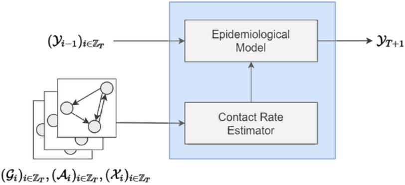
Fig. 1 shows an high level visualization of the proposed architecture. Our model is mainly made up of two building blocks: a Contact Rate Estimator and an Epidemiological Layer, which will be detailed hereunder.

Fig. 1.

High level visualization of the proposed architecture.

Contact Rate Estimator.

It jointly exploits structured data and temporal information to estimate the contact rate at time $t$.

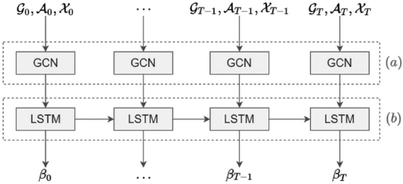
As shown in Fig. 2a, at first we use the historical time series data of graphs and place features as input and a Graph Convolutional Network (GCN) captures the topological structure of the network of places and provides an embedding for each place of the network at time $t$; the obtained time series of node embeddings representing the spatial features of the graph is the input of a Long Short Term-Memory (LSTM) model (see Fig. 2b) whose aim is to capture the temporal features related to dynamic changes in the graph topology, hence returning the sequence of contact rate arrays ${\left({\beta }_i\right)}_{i\in {\mathbb{Z}}_T}$, where each contact rate array ${\beta }_t\in {\mathbb{R}}^{\left|P\right|}$ characterizes each place at time $t$.

Fig. 2.

Contact rate estimator.

The chief reason for the use of a recurrent neural network is the unpredictability of the amount of time that must elapse to see a change in epidemic trends. In other words, the contact rate ${\beta }_t$ at time $t$ has to encapsulate the history of the interactions between individuals which could lead to a change of epidemic trends at time $t+1$.

Epidemiological Model. It predicts the evolution of the epidemic based on previous data and parameters learned by the neural network.

As shown in Fig. 3, the epidemiological layer requires an initial state and the dynamically-changing values of the contact rate for each place, allowing it to compute the intermediate and final results.

Fig. 3.

Epidemiological layer.

For example, a standard approach to epidemic modeling is the SIR compartmentalized model, where each time step $t$ for each place $p$ is characterized by the number of Susceptible ($S_t^p$), Infected ($I_t^p$) and Recovered ($R_t^p$) individuals. Supposing that $R_0^p=0$ and $S_0^p=N^p-I_0^p$, $N^p$ being the number of inhabitants of place $p$ and $I_0^p$ the initial number of infections (provided by the user), the evolution of the epidemic is caught by the following equations:

$$S_{t+1}^p=S_t^p-\frac{{\beta }_t^p{S}_t^p{I}_t^p}{N^p}\left(\left(6\right)\right)$$

$$I_{t+1}^p=I_t^p+\frac{{\beta }_t^p{S}_t^p{I}_t^p}{N^p}-{\gamma }^p{I}_t^p\left(\left(7\right)\right)$$

$$R_{t+1}^p=R_t^p+{\gamma }^p{I}_t^p,\left(\left(8\right)\right)$$

where ${\beta }_t^p$ is the contact rate returned by the Contact Rate Estimator module, and ${\gamma }^p$ is the recovery rate of place $p$. In theory, the recovery rate should not be much different between nearby places, but in practice it is, since the modalities of population testing (e.g., number of swabs) and epidemic handling (e.g., treatment of patients) differ from place to place. In the proposed model, recovery rates can be treated as constants estabilished a-priori by medical reporting or as trainable parameters.

5. Case Study: The COVID-19 Outbreak in Italy

We implemented our methodology using Pytorch and its library PyTorch-geometric [44] and evaluated the results with different compartimental models using Italian data from the 24th February to the 4th May; in particular, the models have been trained considering the fraction of the infected, recovered, deceased populations. We conducted both regional and provincial analysis. The code is publicly available on github.³

5.1. Dataset Description

We have integrated different data sources with the aim of combining mobility data and disease-related information. Table 1 summarizes the features and the labels of the dataset, considering also the granularity level of the available information. Moreover, Table 2 reports some statistics about the regional and the provincial data sets.

TABLE 1. Dataset Description.

	Features	Description	Granularity
	Infected	The cumulative number of positive patients inclunding recovered and dead ones	Regional, provincial
	Isolated	The cumulative number of asymptomatic patients or symptomatic with mild symptoms	Regional
Labels	Hospitalized	The cumulative number of sympomatic patients with serious symptoms	Regional
	ICU	The cumulative number of symptomatic patients in the ICUs	Regional
	Discharged	The cumulative number of recovered patients	Regional
	Deceased	The cumulative number of dead patients	Regional
	#Inhabitants	Population size	Regional, provincial
Static	Population density	Population size per unit area	Regional, provincial
features	Good health (%)	Percentage of healthy people	Regional
	Chronic disease (%)	Percentage of people at least one chronic disease	Regional
	#Arrivals/Departures	Number of arrivals/departures in 2017 considering air travel	Regional
	Non-travelling (%)	Fraction of people who stay at home	Regional, provincial
Dynamic	Incoming (%)	Fraction of people who enter in a city/region	Regional, provincial
features	Radius of gyration	Median distance to which people spep away	Regional, provincial
	#Swab tests	Number of Swab tests	Regional
Edge features	Flows score	Index of mobility between two cities/regions	Regional, provincial

TABLE 2. Dataset Statistics.

Statistic	Regional dataset	Provincial dataset
#Graphs	72	72
#Nodes	20	87
#Features	16	9
#Labels	4	1
#Edges (average)	68	358

Data about the spread of the Covid-19 across Italian regions and provinces have been made available by the Civil Protection Department.⁴ In particular, regional data provides a much wider outlook of what happened since the number of infections is further characterized considering whether the patients are hospitalized or not, and the severity of their symptoms. Furthermore, the number of swab tests have been published to quantify the control activities that the government is making in order to deal with the disease.

We modeled the graphs nodes using two kinds of data: static features represent urban demography of regions/provinces (e.g., number of inhabitants, population density); dynamic features have been collected using data of COVID-19 Mobility Monitoring project [45] which measures, at provinces level, the fraction of non-travelling users, the fraction of incoming users and the radius of gyration from the 22th February to the 13th March. We have replicated data of the week between 7th and 13th March until the 4th May based on the assumption that no significant changes would be observed because Italian government has extended the lock-down until that date. Moreover, data about swabs tests has been considered dynamic features, as well.

Finally, the graphs’ edges have been weighted using flows data between all Italian places, aggregated at the level of interest, provided by mobile operators.

5.2. Modeling the Epidemic Evolution

Aiming to make most of the data provided by the Civil Protection Department, we conducted our analysis based on two granularity levels: regions and provinces. The thoroughness of the regional-level data (e.g., number of infected, hospitalized, admitted to ICUs, quarantined and recovered individuals) allows us to leverage sophisticated epidemiological models, while the lack of information at provincial-level forces us to settle for simpler models such as SIR.

In the following, we will discuss results obtained with SIRD and SIR epidemiological models on regional and provincial graphs, respectively.

Region Level. SIRD model, differently from SIR, discriminates between healed (Recovered) and Deceased individuals. Data provided by the Civil Protection Department allow us to fit the parameters of this model, making them vary over time and exploiting our Contact Rate Estimator to predict the contact rate due to movements and contacts among the population.

The model learns the dynamically changing values of the contact rate $\beta$ and the recovery and mortality rates $\gamma$ and $\mu$ thanks to the mobility data and the epidemic trends. Fig. 4, which shows the fitting of the model for predicting Infected, Recovered and Deceased cases compared to the ground truth, demonstrates the suitability of the proposed architecture.

Fig. 4.

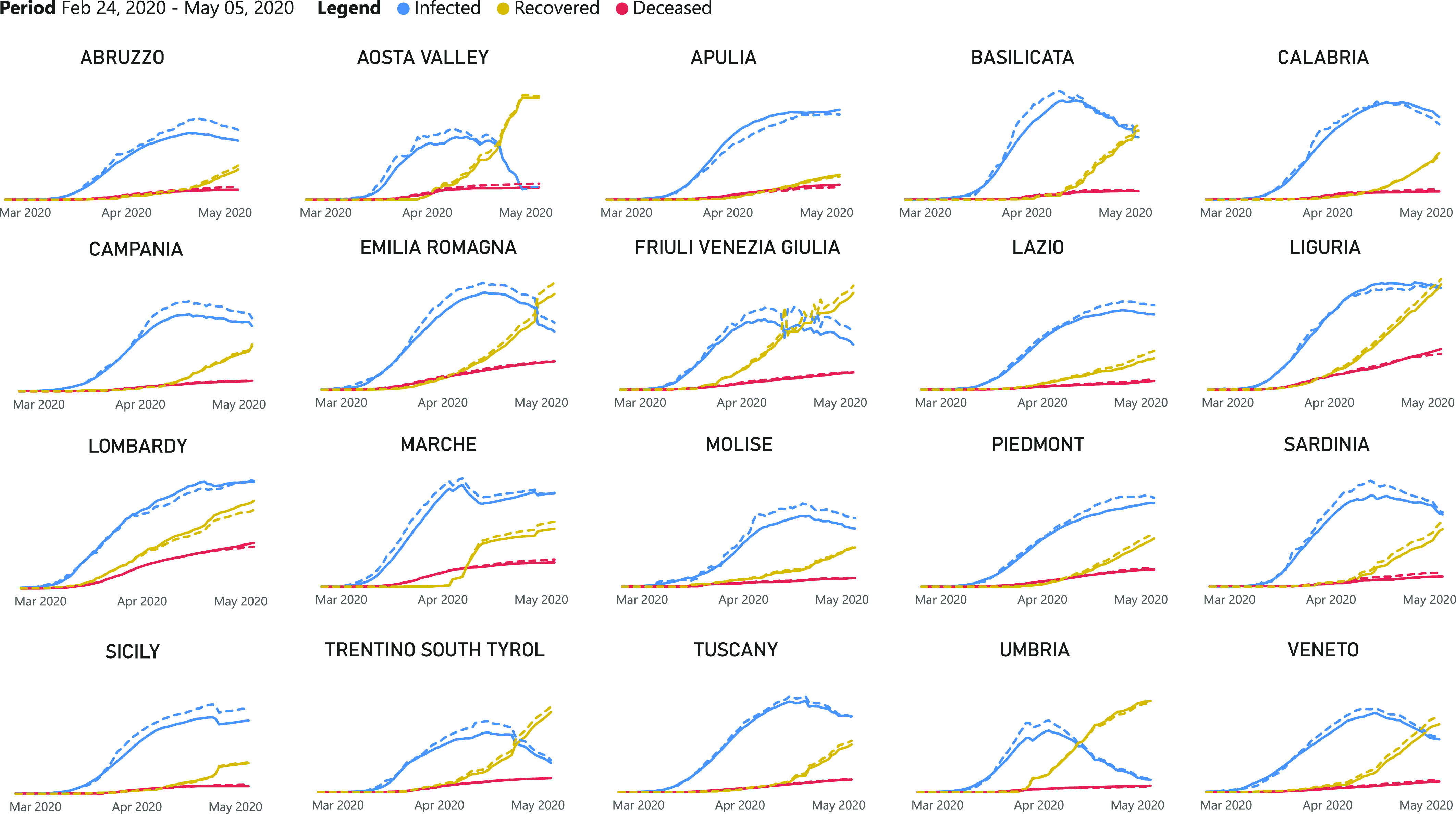
Fitting of the model for predicting Infected, Recovered and Deceased cases compared to the ground truth.

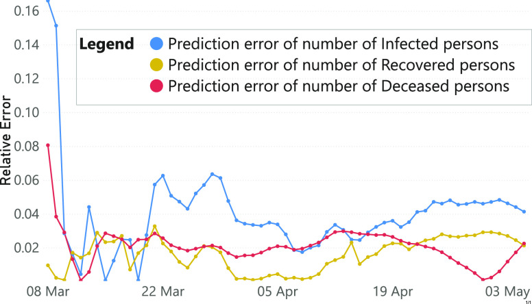
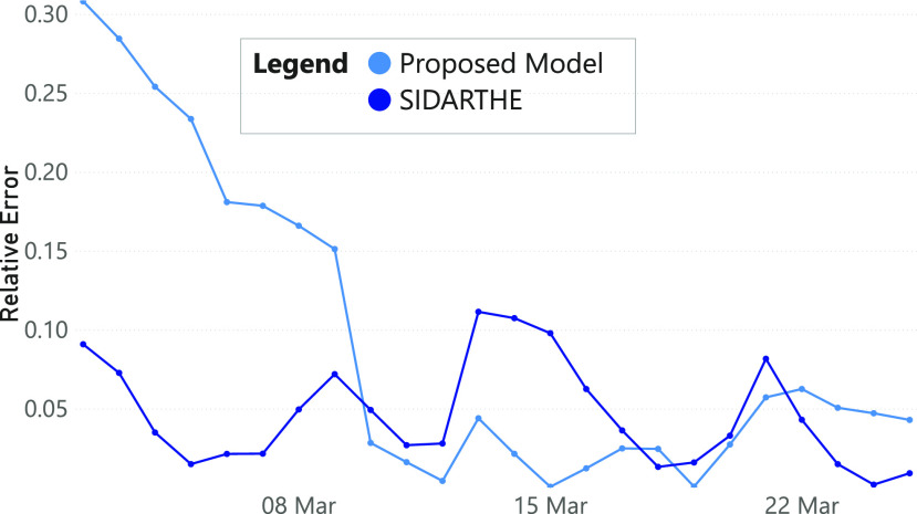
We further evaluate the prediction accuracy of our model in Fig. 5. We summed predictions of Italian regions and computed the relative errors compared to the ground truth since the lock-down. The resulting error rates, being below the 6 percent, demonstrate the appropriateness of our framework. We also compared our model with SIDARTHE [28], a compartmental model designed and implemented to be applied to the pandemic under consideration (refer to Fig. 6). The infected predictions’ results suggest that, after a first period in which data about movements are not enough to catch up the performance of SIDARTHE, our model achieves similar or even better results. A possible improvement of our framework, related to its application on the COVID-19 pandemic, could be represented by the use of SIDARTHE, or other task-specific mathematical models, on top of our Contact Rate Estimator.

Fig. 5.

Relative errors of the prediction of the number of infected, recovered and deceased persons, averaged over Italian regions.

Fig. 6.

Relative errors of the number of infected persons compared with SIDARTHE.

The dynamically changing values of contact rates are shown in Fig. 7, which highlights a huge decrease in contacts between individuals after the beginning of the lock-down.

Fig. 7.

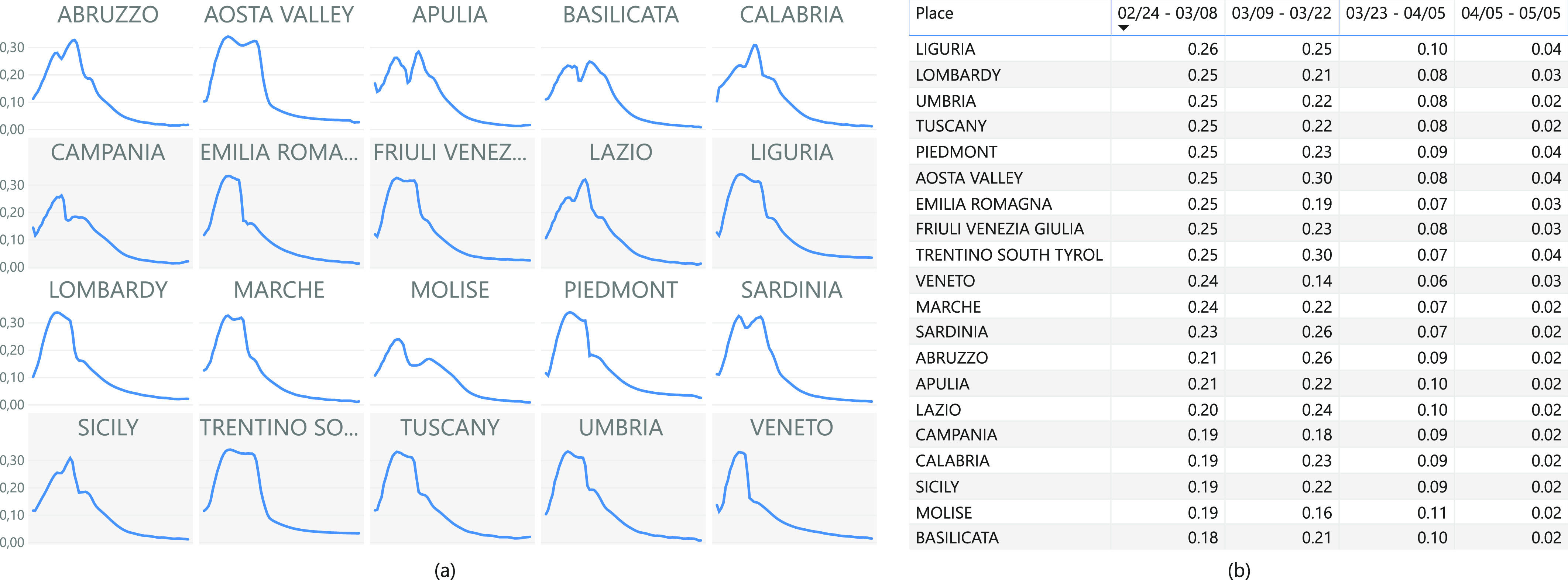
Analysis of the contact rates for Italian regions: (a) Evolution between 24th February and 4th May, (b) average value of concact rates considering a time windows of 14 days.

Province Level. As shown in Table 1, Civil Protection Department only published data about the total number of positive cases for each province. This limitation has prevented us to employ more sophisticated compartmental frameworks than the classical SIR model.

The system has been configured so as to optimize the sum between the infected (I) and recovered (R) people. In particular, the model learns the contact rate ${\beta }_p^t$ and the recovery rate ${\gamma }_p$ for each province $p$ and time interval $t$.

Fig. 8 shows the comparison between the predicted cases and the real ones, for brevity just a subset of 20 provinces is depicted. The model has been able to learn always the first part of the time series while the few errors in the second part probably depend by the increased number of recovered people with respect to that of the (new) infected ones.

Fig. 8.

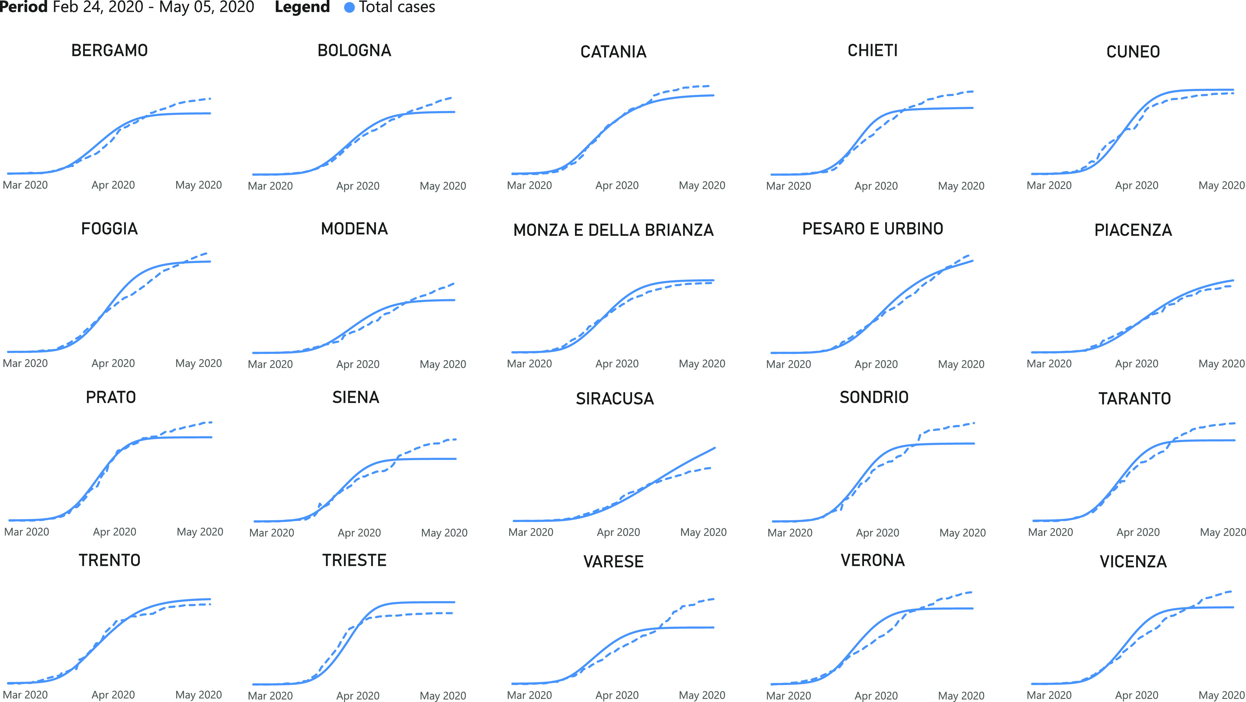
Comparison between the infection cases predicted by the proposed model and the real ones over a subset of Italian provinces.

Fig. 9 outlines the estimated series of basic reproduction numbers $R_{0_p}^t={\beta }_p^t/{\gamma }_p$ for each province $p$. Their behavior represents the effectiveness of social distancing countermeasures taken by national and regional governments: in fact they have quickly increased until the first week of March when no action has been taken yet, and started decreasing from the end of March, once the lock-down policy, adopted on the 9th, had taken effect. Specifically, the epidemic threshold $R_0=1$ has been reached at the beginning of April for all provinces, meaning that, regardless the different number of infectious, the disease spreading has been controlled over the national territory.

Fig. 9.

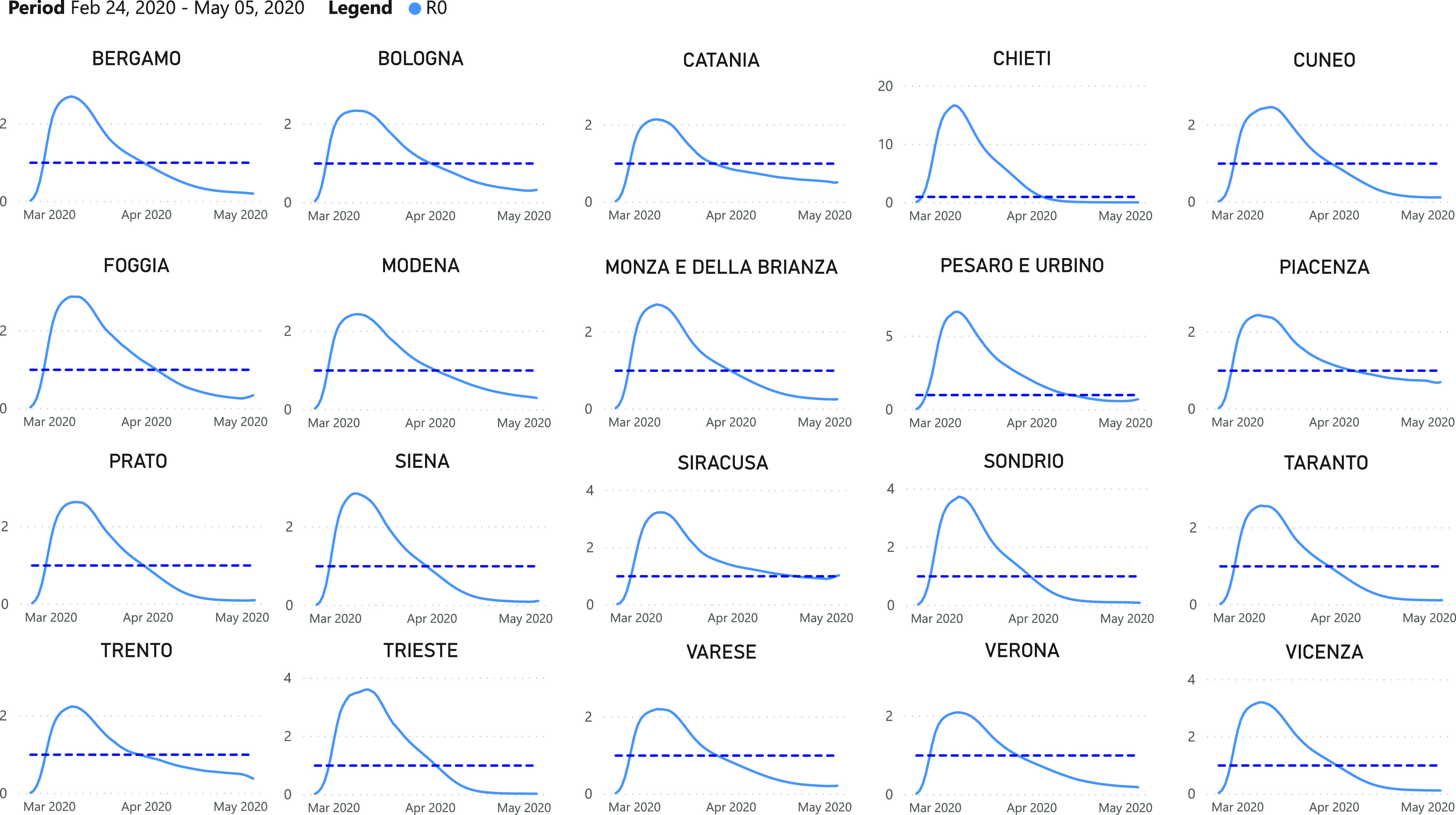
Estimated series of basic reproduction numbers $R_{0_p}^t={\beta }_p^t/{\gamma }_p$ for each province $p$.

5.3. Forecasts and What-If Analysis

The epidemiological model at the top of the proposed architecture can be easily used as a standalone model which allows us to project forecasts about the future of the epidemic.

Figs. 10a and 10b report what would have happened to the number of infections after the 5th May if the contact rate among individuals changed (decreased or increased, respectively) within the four Italian regions most affected by the pandemic (i.e., Lombardy, Emilia Romagna, Piedmont, Veneto).

Fig. 10.

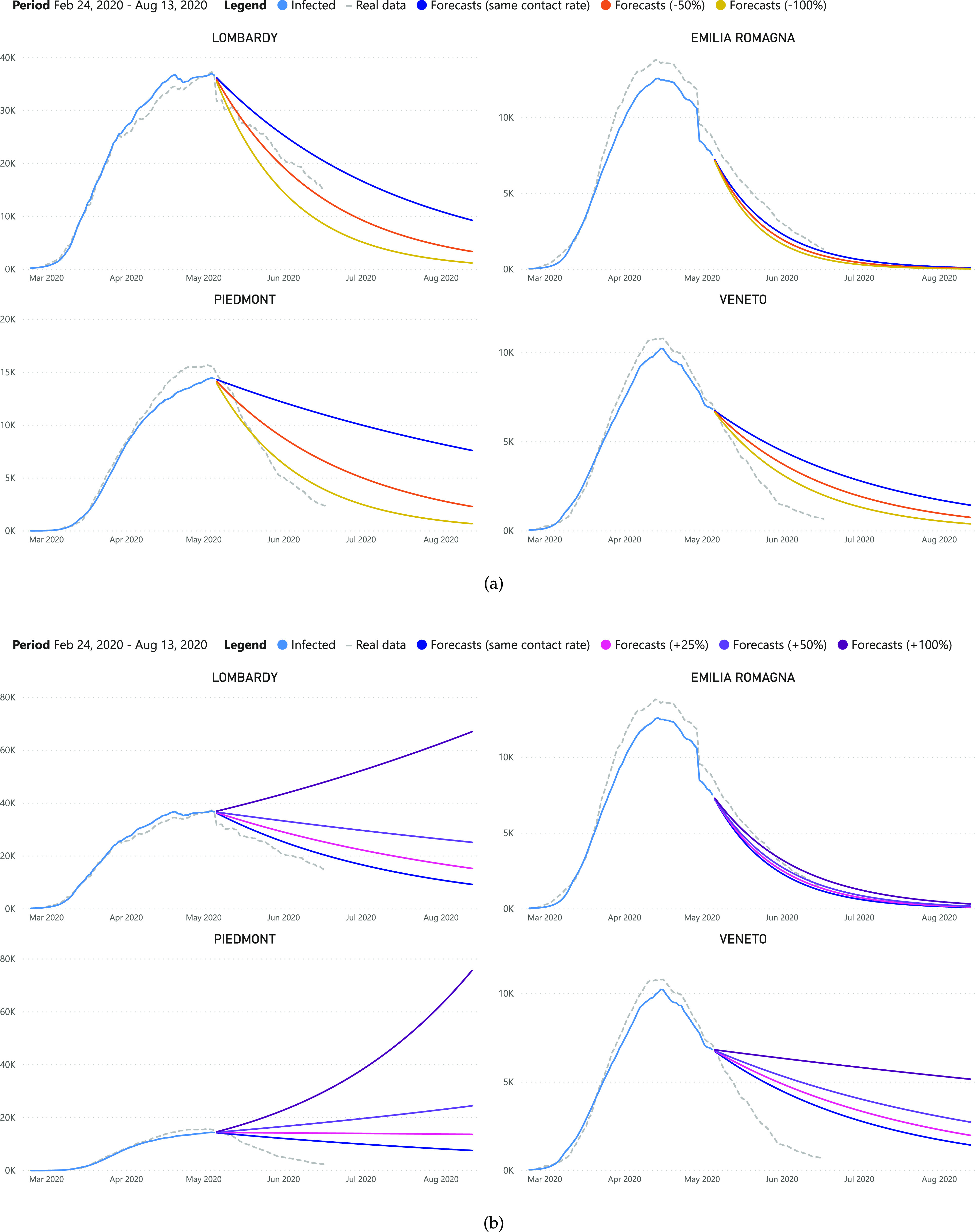
Analysis of the predicted total number of infected individuals by decreasing (a) and increasing (b) the contact rate after May 5th.

Results reveal that the real trend of infections, in the majority of cases, is more descending than the one predicted by the model, thanks to a lower contact rate and/or a higher recovery/mortality rate. Moreover, according to the forecasts, increases of contact rate could cause dramatic new waves of infections, in some regions (e.g., Piedmont, Lombardy) more than others.

6. Conclusions and Future Work

In this paper, we proposed a novel machine learning based framework able to estimate parameters of an epidemiological model fitting epidemiological trends on the basis of users’ mobility data.

The main characteristics of the proposed approach are: i) to model epidemic spread by means of time-variant graph in which nodes represent places where infection can take place, and edges represent users movements between two places; ii) to exploit GCNs and LSTMs in order to infer the model parameters on the basis of different and successive temporal snapshots of the epidemic graph.

We evaluated the proposed approach using data related to the COVID-19 outbreak in Italy, integrating mobility data provided by network service providers and infection statistics crawled from several sources (i.e., ISTAT and humdata). In particular, we compare the forecasts of the trained model with real data on the epidemic and obtaining promising result: not only does the model predict the contagion curve despite the number of places graphs are formed, but also its performance is comparable with the ones of complex compartmental models. Moreover, the training procedure learns jointly the diffusion process and the best parameters for the on-top epidemiological model, enabling further ”post-hoc” analysis on how some countermeasures have affected the disease's spread. Finally, we simulate what could have happened after May 5th, analyzing the predicted total number of infected individuals by decreasing and increasing the contact rate.

Future works will be devoted to enrich our epidemic graph with further information (demographic, logistics, attractions, etc.) and to study how such data can improve model predictions. We would like to investigate how to customize the GCN module to get a better modeling of the characteristics of epidemic spreading. Finally, our aim is also to investigate how eXplainable Artificial Intelligence (XAI) techniques can be used to infer which features and/or movements have influenced more the model prediction.

Biographies

Valerio La Gatta received the master's degree in computer engineering from the University of Naples Federico II, in 2020. He is currently a research fellow at the Consorzio Interuniversitario Nazionale per l'informatica (CINI). His research interests include at social network analysis, multimedia analysis, and eXplainable Artificial Intelligence.

Vincenzo Moscato received the PhD degree in computer science and engineering from the University of Naples “Federico II”. He is currently an associate professor of Database and Information Systems with the Department of Electrical Engineering and Information Technologies, University of Naples “Federico II”. He has been active in the field of computer vision, video and image indexing, multimedia data sources integration and recommender systems. His current research interests include the area of multimedia, knowledge management and Big Data analytics. He was involved in several international, national and local research projects and at present is an author of more than one hundred publications on international journal and conference proceedings.

Marco Postiglione received the master's degree in computer engineering from the University of Naples Federico II, in 2020. He is a research fellow with the Consorzio Interuniversitario Nazionale per l'informatica (CINI). His research interests include focused on eXplainable Artificial Intelligence, Social Network Analysis and Multimedia Analysis.

Giancarlo Sperlí received the PhD degree in information technology and electrical engineering from the University of Naples ”Federico II” defending his thesis: “Multimedia Social Networks”. He is a research fellow with the Department of Electrical and Computer Engineering, University of Naples ”Federico II”. He is a member of the MISLAB (Multimedia Information System LABoratory) and PRIAMUS (Pattern Recognition, Image Analysis and Multimedia Systems) departmental research groups. His main research interests include the area of Cybersecurity, Semantic Analysis of Multimedia Data and Social Networks Analysis. Finally, he has authored about 50 publications in international journals, conference proceedings and book chapters.

References

- [1].Rodriguez-Morales A. J., et al. , “Clinical, laboratory and imaging features of covid-19: A systematic review and meta-analysis,” Travel Med. Infectious Disease, 2020, Art. no. 101623. [Online]. Available: http://www.sciencedirect.com/science/article/pii/S1477893920300910 [DOI] [PMC free article] [PubMed]
- [2].Singhal T., “A review of coronavirus disease-2019 (COVID-19),” Indian J. Pediatrics, vol. 87, pp. 281–286, 2020. [DOI] [PMC free article] [PubMed] [Google Scholar]
- [3].Ralph R., et al. , “2019-nCov (wuhan virus), a novel coronavirus: Human-to-human transmission, travel-related cases, and vaccine readiness,” J. Infection Developing Countries, vol. 14, no. 1, Jan. 2020, Art. no. 3—17. [Online]. Available: https://doi.org/10.3855/jidc.12425 [DOI] [PubMed] [Google Scholar]
- [4].Kwok K. O., Tang A., Wei V. W., Park W. H., Yeoh E. K., and Riley S., “Epidemic models of contact tracing: Systematic review of transmission studies of severe acute respiratory syndrome and middle east respiratory syndrome,” Comput. Structural Biotechnol. J., vol. 17, pp. 186–194, 2019. [DOI] [PMC free article] [PubMed] [Google Scholar]
- [5].Guan W.-j., et al. , “Clinical characteristics of coronavirus disease 2019 in china,” New England J. Med., vol. 382, pp. 1708–1720, 2020. [Online]. Available: https://doi.org/10.1056/NEJMoa2002032 [DOI] [PMC free article] [PubMed] [Google Scholar]
- [6].Tillett H. E., “Infectious diseases of humans: Dynamics and control,” Epidemiol. Infection, vol. 108, 1992, pp. 211–211. [Google Scholar]
- [7].Diekmann O. and Heesterbeek J., Mathematical Epidemiology of Infectious Diseases: Model Building, Analysis and Interpretation, Hoboken, NJ, USA: Wiley, 2000. [Google Scholar]
- [8].Hethcote H., “The mathematics of infectious diseases,” SIAM Rev., vol. 42, pp. 599–653, 2000. [Google Scholar]
- [9].Brauer F. and Castillo-Chávez C., Mathematical Models in Population Biology and Epidemiology, vol. 40, Berlin, Germany: Springer, 2001. [Google Scholar]
- [10].William Ogilvy K. and McKendrick A. G., “A contribution to the mathematical theory of epidemics,” in Proc. R. Soc. London Ser. A, Containing Papers Math. Physical Character, 1927, vol. 115.772, pp. 700–721. [Google Scholar]
- [11].Moran K., et al. , “Epidemic forecasting is messier than weather forecasting: The role of human behavior and internet data streams in epidemic forecast downloaded from,” J. Infectious Diseases, vol. 214, pp. 404–412, 2016. [DOI] [PMC free article] [PubMed] [Google Scholar]
- [12].Sahneh F. D., Vajdi A., Melander J., and Scoglio C. M., “Contact adaption during epidemics: A multilayer network formulation approach,” IEEE Trans. Netw. Sci. Eng., vol. 6, no. 1, pp. 16–30, Jan.–Mar. 2017. [DOI] [PMC free article] [PubMed] [Google Scholar]
- [13].Fenichel E., et al. , “Adaptive human behavior in epidemiological models,” Proc. Nat. Acad. Sci. U.S.A., vol. 108, pp. 6306–11, 2011. [DOI] [PMC free article] [PubMed] [Google Scholar]
- [14].Liu M., Liz E., and Röst G., “Endemic bubbles generated by delayed behavioral response: Global stability and bifurcation switches in an sis model,” SIAM J. Appl. Math., vol. 75, pp. 75–91, 2015. [Google Scholar]
- [15].Brauer F., “A simple model for behaviour change in epidemics,” BMC Public Health, vol. 11 Suppl 1, 2011, Art. no. S3. [DOI] [PMC free article] [PubMed] [Google Scholar]
- [16].Darabi Sahneh and F., Scoglio C., “Epidemic spread in human networks,” in Proc. 50th IEEE Conf. Decis. Control Eur. Control Conf., 2011, pp. 3008–3013. [Google Scholar]
- [17].Darabi Sahneh F., Chowdhury F., and Scoglio C., “On the existence of a threshold for preventive behavioral responses to suppress epidemic spreading,” Sci. Reports, vol. 2, 2012, Art. no. 632. [DOI] [PMC free article] [PubMed] [Google Scholar]
- [18].Zuo L. and Liu M., “Effect of awareness programs on the epidemic outbreaks with time delay,” Abstract Appl. Anal., vol. 2014, pp. 1–8, 2014. [Google Scholar]
- [19].Obermeyer Z. and Emanuel E. J., “Predicting the future - big data, machine learning, and clinical medicine,” New England J. Med., vol. 375 13, pp. 1216–1219, 2016. [DOI] [PMC free article] [PubMed] [Google Scholar]
- [20].Yang Z., et al. , “Modified seir and ai prediction of the epidemics trend of COVID-19 in china under public health interventions,” J. Thoracic Disease, vol. 12, no. 3, 2020, Art. no. 165. [DOI] [PMC free article] [PubMed] [Google Scholar]
- [21].Soures N., et al. , “SIRNet: Understanding social distancing measures with hybrid neural network model for COVID-19 infectious spread,” 2004, arXiv: 2004.10376.
- [22].Bogoch I. I., Watts A., Thomas-Bachli A., Huber C., Kraemer M. U. G., and Khan K., “Pneumonia of unknown aetiology in Wuhan, China: Potential for international spread via commercial air travel,” J. Travel Med., vol. 27, no. 2, 2020. [Online]. Available: https://doi.org/10.1093/jtm/taaa008 [DOI] [PMC free article] [PubMed] [Google Scholar]
- [23].Li L., et al. , “Characterizing the propagation of situational information in social media during COVID-19 epidemic: A case study on weibo,” IEEE Trans. Comput. Soc. Syst., vol. 7, no. 2, pp. 556–562, Apr. 2020. [Google Scholar]
- [24].Chen Y.-C., Lu P.-E., and Chang C.-S., “A time-dependent SIR model for COVID-19,” 2020, arXiv: 2003.00122. [DOI] [PMC free article] [PubMed]
- [25].Dolbeault J. and Turinici G., “Heterogeneous social interactions and the COVID-19 lockdown outcome in a multi-group seir model,” 2020, arXiv: 2005.00049.
- [26].Zhong L., Mu L., Li J., Wang J., Yin Z., and Liu D., “Early prediction of the 2019 novel coronavirus outbreak in the mainland china based on simple mathematical model,” IEEE Access, vol. 8, pp. 51 761–51 769, 2020. [DOI] [PMC free article] [PubMed] [Google Scholar]
- [27].Dehning J., et al. , “Inferring COVID-19 spreading rates and potential change points for case number forecasts,” 2020, arXiv: 2004.01105.
- [28].Giordano G., et al. , “Modelling the COVID-19 epidemic and implementation of population-wide interventions in Italy,” Nat. Med., Apr. 2020. [Online]. Available: http://dx.doi.org/10.1038/s41591-020-0883-7 [DOI] [PMC free article] [PubMed]
- [29].Seo Y., Defferrard M., Vandergheynst P., and Bresson X., “Structured sequence modeling with graph convolutional recurrent networks,” in Proc. Int. Conf. Neural Inf. Process., 2018, pp. 362–373.
- [30].Manessi F., Rozza A., and Manzo M., “Dynamic graph convolutional networks,” CoRR, vol. abs/1704.06199, 2017. [Online]. Available: http://arxiv.org/abs/1704.06199
- [31].Pareja A., et al. , “Evolvegcn: Evolving graph convolutional networks for dynamic graphs,” CoRR, vol. abs/1902.10191, 2019. [Online]. Available: http://arxiv.org/abs/1902.10191 [Google Scholar]
- [32].Kipf T. N. and Welling M., “Semi-supervised classification with graph convolutional networks,” CoRR, vol. abs/1609.02907, 2016. [Online]. Available: http://arxiv.org/abs/1609.02907
- [33].Xu D., Zhu Y., Choy C. B., and Fei-Fei L., “Scene graph generation by iterative message passing,” CoRR, vol. abs/1701.02426, 2017. [Online]. Available: http://arxiv.org/abs/1701.02426
- [34].Yang J., Lu J., Lee S., Batra D., and Parikh D., “Graph R-CNN for scene graph generation,” CoRR, vol. abs/1808.00191, 2018. [Online]. Available: http://arxiv.org/abs/1808.00191 [Google Scholar]
- [35].Veličković P., Cucurull G., Casanova A., Romero A., Liò P., and Bengio Y., “Graph attention networks,” 2017, arXiv:1710.10903.
- [36].Duvenaud D., et al. , “Convolutional networks on graphs for learning molecular fingerprints,” CoRR, vol. abs/1509.09292, 2015. [Online]. Available: http://arxiv.org/abs/1509.09292 [Google Scholar]
- [37].Gilmer J., Schoenholz S. S., Riley P. F., Vinyals O., and Dahl G. E., “Neural message passing for quantum chemistry,” CoRR, vol. abs/1704.01212, 2017. [Online]. Available: http://arxiv.org/abs/1704.01212 [Google Scholar]
- [38].Graves A., Supervised Sequence Labelling. In Supervised Sequence Labelling with Recurrent Neural Networks, Springer, Berlin, Heidelberg, 2012, pp. 5–13. [Google Scholar]
- [39].Graves A., Mohamed A. R., and Hinton G., “Speech recognition with deep recurrent neural networks,” in Proc. IEEE Int. Conf. Acoust., Speech Signal Process., 2013, pp. 6645–6649.
- [40].Informatik F., Bengio Y., Frasconi P., and Schmidhuber J., “Gradient flow in recurrent nets: The difficulty of learning long-term dependencies,” Field Guide to Dynamical Recurrent Neural Netw., 2003.
- [41].Hochreiter S. and Schmidhuber J., “Long short-term memory,” Neural Comput., vol. 9, no. 8, Nov. 1997, pp. 1735–1780. [Online]. Available: https://doi.org/10.1162/neco.1997.9.8.1735 [DOI] [PubMed] [Google Scholar]
- [42].Gers F. A., Schmidhuber J. A., and Cummins F. A., “Learning to forget: Continual prediction with LSTM,” Neural Comput., vol. 12, no. 10, Oct. 2000, pp. 2451–2471. [Online]. Available: https://doi.org/10.1162/089976600300015015 [DOI] [PubMed] [Google Scholar]
- [43].Cho K., et al. , “Learning phrase representations using RNN encoder-decoder for statistical machine translation,” in Proc. Conf. Empir. Methods Natural Lang. Process., 2014, pp. 1724–1734. [Google Scholar]
- [44].Fey M. and Lenssen J. E., “Fast graph representation learning with PyTorch Geometric,” in Proc. ICLR Workshop Representation Learn. Graphs Manifolds, 2019, pp. 1–9. [Google Scholar]
- [45].Pepe E., et al. , “Covid-19 outbreak response: A first assessment of mobility changes in italy following national lockdown,” medRxiv, 2020. [Online]. Available: https://www.medrxiv.org/content/early/2020/04/07/2020.03.22.20039933 [DOI] [PMC free article] [PubMed]