STALLION: a stacking-based ensemble learning framework for prokaryotic lysine acetylation site prediction

Abstract

Protein post-translational modification (PTM) is an important regulatory mechanism that plays a key role in both normal and disease states. Acetylation on lysine residues is one of the most potent PTMs owing to its critical role in cellular metabolism and regulatory processes. Identifying protein lysine acetylation (Kace) sites is a challenging task in bioinformatics. To date, several machine learning-based methods for the in silico identification of Kace sites have been developed. Of those, a few are prokaryotic species-specific. Despite their attractive advantages and performances, these methods have certain limitations. Therefore, this study proposes a novel predictor STALLION (STacking-based Predictor for ProkAryotic Lysine AcetyLatION), containing six prokaryotic species-specific models to identify Kace sites accurately. To extract crucial patterns around Kace sites, we employed 11 different encodings representing three different characteristics. Subsequently, a systematic and rigorous feature selection approach was employed to identify the optimal feature set independently for five tree-based ensemble algorithms and built their respective baseline model for each species. Finally, the predicted values from baseline models were utilized and trained with an appropriate classifier using the stacking strategy to develop STALLION. Comparative benchmarking experiments showed that STALLION significantly outperformed existing predictor on independent tests. To expedite direct accessibility to the STALLION models, a user-friendly online predictor was implemented, which is available at: http://thegleelab.org/STALLION.

Introduction

The final step of the ‘central dogma’ of molecular biology is the translation process, where RNA codes for specific proteins [1]. Protein post-translational modifications (PTMs) are important owing to their implications in several biological processes, including cell cycle modulation, DNA repair, gene activation, gene regulation and signaling processes. PTMs are reversible or irreversible chemical changes that occur in the later stages of protein biosynthesis [2, 3]. PTMs can occur in a single amino acid residue or multiple residues resulting in changes in the chemical properties of altered sites [4]. Reversible modifications include covalent modifications, whereas irreversible changes include proteolytic modifications [5]. PTMs can affect several properties of proteins, such as cell–cell/cell–matrix interactions, enzyme assembly and function, molecular trafficking, protein–protein interactions (PPIs), protein folding, protein localization, protein solubility, protein lifespan and receptor activation, thus acting as an important regulatory tool in protein function [6, 7]. Over 400 different types of PTMs have been identified ranging from the addition of small chemical or complex groups (viz. acetylation, methylation, phosphorylation, etc.) to the addition of polypeptides (viz. ubiquitylation and SUMOylation; [8]). The lysine residue undergoes the largest number of PTMs with at least 15 PTM types [8]. According to the dbPTM database statistics, phosphorylation, acetylation and ubiquitination are the three major types that cover >90% of reported PTMs [9].

Lysine acetylation (Kace) is one of the most important ubiquitous PTMs and is highly conserved in both prokaryotes and eukaryotes [10]. This modification is a covalent PTM catalyzed by lysine acetyl transferases (KATs), where the acetyl group (CH₃CO) from acetyl coenzyme A is transferred to either the free α-amino group (NH₃⁺) of the N-terminal residue (Nα-acetylation) or to the ε-amino group of internal lysine (Nε-acetylation) at specific sites [11]. Acetylation is of three types, viz. Nα-, Nε- and O-acetylation. Nε- and O-acetylations are reversible modifications, whereas Nα-acetylation is an irreversible one [12]. Nα-acetylation is common in eukaryotes [13], whereas Nε-acetylation is more biologically substantial, playing prominent roles in actin nucleation, cell cycle regulation, chromatin stability, cell metabolism, nuclear transport and PPIs [14]. Dysregulation of Kace has also been linked to aging and several diseases including cancer, immune disorders and cardiovascular and neurological diseases [15, 16]. Given that acetylation is important in cell biology and disease pathologies, identifying Kace sites is necessary for understanding its modulatory mechanism.

Recently, several experimental methods, including radioactivity chemical methods, mass spectrometry and chromatin immunoprecipitation, have been developed to detect Kace PTM sites [17]. Owing to the latest innovations in science and technology, our ability to detect Kace sites has improved drastically; however, considering the proteome size, we have only uncovered a minute portion of the lysine ‘modifyome’. Moreover, testing every lysine residue in a single protein is laborious. The intricacies involved in the experimental identification of Kace sites (time-consuming, expensive, labor intensive and low throughput) have led to a plethora of computational approaches devised to predict potential candidates for experimental validation, particularly machine learning (ML) tools, which have become increasingly prevalent for their speedy and accurate predictions. In the last decade, several ML techniques have been developed to identify Kace sites in prokaryotes and eukaryotes [18–22].

Currently, more than a dozen Kace prediction tools are available, such as PAIL [23], LysAcet [24], EnsemblePail [25], N-Ace [26], BPBPHKA [27], PLMLA [28], PSKAcePred [29], KAcePred [31], LAceP [31], AceK [32], SSPKA [33], iPTM-mLys [34], KA-predictor [35], ProAcePred [36], ProAcePred 2.0 [37], Ning et al. [38] and DNNAce [39]. Most predictors were designed for identifying acetylation in eukaryotes and lacked species specificity. However, there are a few existing predictors that have been developed for identifying Kace in prokaryotes. SSPKA and KA-predictor were developed for both eukaryotic and prokaryotic acetylation site predictions, which included two prokaryotes, Escherichia coli and Salmonella typhimurium, thus underscoring the importance and necessity of a species-specific model. Chen et al. [36] developed a predictor called ProAcePred for nine prokaryotic species, Archaea, Bacillus subtilis, Corynebacterium glutamicum, Erwinia amylovora, E. coli, Geobacillus kaustophilus, Mycobacterium tuberculosis, S. typhimurium and Vibrio parahemolvticus. Later, the same group [36] developed the updated version of ProAcePred predictor called ProAcePred 2.0 [37] for six prokaryotic species: B. subtilis, C. glutamicum, E. coli, G. kaustophilus, M. tuberculosis and S. typhimurium. The training dataset was marginally larger than utilized in ProAcePred. Such ML studies provide an opportunity to understand differences in substrate site specificity between prokaryotic and eukaryotic species.

Although progress has been made in the computational prediction of Kace sites, a few limitations need to be addressed. First, most of the state-of-the-art approaches used simple ML algorithms such as support vector machine (SVM) or random forest (RF) to train the model. Owing to the advancement in cutting-edge technologies, advanced ML approaches, such as deep learning (DL) [40, 41], iterative feature representation [42] or ensemble-based stacking approach [43, 44], could be utilized for developing a more robust and stable predictor to enhance the predictive performance of Kace sites. Second, the feature space used by the existing methods in Kace prediction is rather limited. Finally, the state-of-the-art methods used simple feature selection technique to identify the optimal feature subset. Unfortunately, such simple approaches may overlook the critical features present in Kace site prediction.

Considering these limitations, we developed a novel stacking-based predictor known as STALLION (STacking-based Predictor for ProkAryotic Lysine AcetyLatION) to enhance the accurate prediction of Kace sites in six different prokaryotic species. Major advantages of our proposed method over other state-of-the-art methods could be summarized as follows: (i) STALLION is the first stacking ensemble-based predictor for the identification of Kace sites in prokaryotes; (ii) We comprehensively evaluated and compared 11 different encoding schemes for each species with an attempt to extract patterns representing a wide range of sequence, position-specific and physicochemical characteristics. Subsequently, we identified optimal feature set using three different computationally intensive approaches separately for five popular tree-based ensemble algorithms and trained the base classifiers and (iii) A stacked-model STALLION was trained with an appropriate classifier using the predicted information from the base classifiers and 5-fold cross-validation. Comparative analysis on independent datasets showed that the STALLION significantly outperformed existing predictor, thus highlighting the significance of utilizing our systematic approach in STALLION for Kace prediction.

Materials and methods

Training and independent datasets

Recently, Chen et al. [37] constructed novel nonredundant datasets, based on the PLMD database [45] (http://plmd.biocuckoo.org), for six species, B. subtilis, C. glutamicum, E. coli, G. kaustophilus, M. tuberculosis and S. typhimurium. Consequently, CD-HIT [46] was applied to eliminate the homologous sequences by setting the threshold of sequence identity to 30%, which is immensely valuable for avoiding overestimation during cross-validation or model training. While constructing the dataset, the authors experimented using different fragment sizes and identified the optimal size as 21-residue-long sequence segments with K at the center. The segments were defined as positive samples (Kace) if the central K residue acetylation was experimentally validated, otherwise they were deemed negative (non-Kace) samples. Notably, central K lacking residues or the gap at either terminus was replaced with a dummy atom ‘O’. Utilizing these datasets, they developed a species-specific Kace site predictor called ProAcePred 2.0.

We utilized the same dataset for the current study because they were recently constructed and used a rigorous approach to identify optimal length. In general, developing a prediction model using such a high-quality dataset may have more comprehensive practical applications [47]. A statistical summary of the training and independent datasets for each species is shown in Table 1. We employed balanced training datasets for prediction model development and imbalanced independent datasets to check the model robustness.

Table 1.

A statistical summary of the training and independent datasets for six species

Species	Positive	Negative	Positive	Negative
E. coli	6592	6592	361	1384
C. glutamicum	1052	1052	83	830
M. tuberculosis	865	865	68	575
B. subtillis	1571	1571	125	1165
S. typhimurium	198	198	10	217
G. kaustophilus	206	206	17	192

Note: The first column represents the species, the second and third columns represent the positive and negative samples of the training dataset, and the fourth and fifth columns represent the positive and negative samples of the independent dataset.

Selection of feature encoding schemes

To create an efficient ML-based method for Kace prediction, several different feature encoding schemes were employed to encode 21 types of amino acids [20 standard amino acids and dummy residues for gap (O)]. In total, we employed 11 encoding schemes that can be grouped into three major types: (i) sequence-based features include numerical representation of amino acid (NRA), binary encoding (BINA), amino acid composition (AAC), dipeptide composition (DPC) and conjoint triad (CTF); (ii) physicochemical properties based features include amino acid index (AAI), grouped dipeptide composition (GDPC), grouped tripeptide composition (GTPC), Composition of k-Spaced Amino Acid Group Pairs (CKSAAGP) and Zscale and (iii) position-specific scoring matrices include BLOSUM62. A brief description of these 11 feature encoding schemes is as follows:

Sequence-based features

Numerical representation for amino acids features (NRF)

In NRF encoding, protein sequences are converted into numerical values [48] by mapping amino acids in an alphabetical order. The 21 amino acids are represented as 0.0–2.0 with an interval of 0.1. We ignored the central K residue from a given 21-residue segment and considered 10 upstream and 10 downstream sequences, resulting in a 20-dimensional (20D) feature vector.

Binary encoding (BINA)

In BINA encoding, each amino acid converts into a segment of a 21D orthogonal binary vector [49]. For example, alanine, cysteine and glutamic acid are represented as [1, 0, 0, 0, 0, 0, 0, 0, 0, 0, 0, 0, 0, 0, 0, 0, 0, 0, 0, 0, 0], [0, 1, 0, 0, 0, 0, 0, 0, 0, 0, 0, 0, 0, 0, 0, 0, 0, 0, 0, 0, 0] and [0, 0, 1, 0, 0, 0, 0, 0, 0, 0, 0, 0, 0, 0, 0, 0, 0, 0, 0, 0, 0], respectively. The dummy amino acid ‘O’ is represented as [0, 0, 0, 0, 0, 0, 0, 0, 0, 0, 0, 0, 0, 0, 0, 0, 0, 0, 0, 0, 1]. Thereafter, we obtained a 441D vector for the given sequence with a length of 21.

Amino acid composition (AAC): AAC computes the frequency of 21 amino acids from the given protein fragment sequence, which has been used as a descriptor for several peptide function predictions [50, 51]. The frequency of each amino acid is normalized into 0–1 by dividing the sequence length. AAC resulted in a 21D feature vector.

Di-peptide composition (DPC)

Twenty-one amino acids generate 441 (21 × 21) dipeptides. DPC computes the percentage of all possible dipeptide combinations from the given sequence, reflecting each protein sequence global information and local order amino acids information. Notably, DPC has been widely applied to capture segmental information around PTMs [52].

Conjoint triad features (CTF)

In CTF, 20 amino acids were categorized into seven classes ({VGA}, {PFLI}, {STMY}, {WQNH}, {RK}, {ED} and {C}) according to their volumes of side chains and dipoles [53]. Notably, we added a dummy atom to the first class {VGAO}. CTF considers the properties of one amino acid and its vicinal amino acids by regarding any three contiguous amino acids as a single unit. A 343D vector represents a given sequence.

Physicochemical properties-based features

Amino acid index (AAI)

AAI is the publicly available database that represents the physicochemical properties of amino acids as the most intuitive features for describing biochemical reactions (https://www.genome.jp/aaindex/; [54]). We utilized 531 physicochemical properties from the database as employed in the previous study [55] and encoded the given sequence.

Grouped di-peptide composition (GDPC)

Each amino acid has a specific physicochemical property. Accordingly, they have been categorized into five different groups: aliphatic (IMLVAG), aromatic (WYF), positively charged (HRK), negatively charged (ED) and uncharged (QNPCTSO). We assigned dummy residue (O) to the uncharged group. By utilizing these five groups, GDPC are classified into 25 classes that result in a 25D feature vector [56, 57].

Grouped tri-peptide composition (GTPC)

In GTPC [58, 59], the tri-peptide composition is classified into 125 classes by employing five categories as mentioned in GDPC, which result in a 125D vector.

Composition of k-spaced amino acid group pairs (CKSAAGP)

The CKSAAGP also calculates the frequency of amino acid pairs separated by k residues (the value of k is 0–5). Unlike the composition of k-spaced amino acid pairs [58], it classifies them into five categories based on the physicochemical properties of amino acids, and subsequently classifies the properties of the dipeptide compositions into 25 categories. Thus, the amino acid pair gives a total of 25 descriptors, and the number of divided residues is 0–5, such that a 150D vector is finally formed.

Z-scale (Zscale)

In Zscale, each amino acid is characterized by five physicochemical descriptor variables, according to Sandberg et al. [59]. A given sequence is converted into 105 (5 × 21) D vector by incorporating these five physicochemical descriptors.

Position-specific scoring matrices

BLOSUM62 (BLOS)

BLOSUM62 matrix is commonly applied in a BLAST sequence alignment program. Here, it was used to convert the protein sequence to describe the similarity of two sequence segments. Generally, this substitution matrix is applied to study sequence conservation of related proteins in large databases, which has been used as features in several predictors [60, 61]. Each row in the BLOSUM62 matrix can be used to encode one of the 20 amino acids. Therefore, we can encode according to the BLOSUM62 matrix, forming a feature vector of 420 (20 × 21) D.

Selection of ML algorithms

In this study, we employed six different classifiers that included five decision-tree-based classifiers (RF [62], extreme gradient boosting algorithm (XGB) [63], AdaBoost (AB) [64], gradient boosting (GB) [65], extremely randomized tree (ERT) [66]) and SVM [67]. Generally, decision-tree-based algorithms can handle unnormalized features unlike other supervised and DL algorithms [68]. Hence, we only employed these five classifiers for the baseline model construction. However, six classifiers were used for meta-model construction and the appropriate one was selected. These classifiers have been widely applied in numerous successful applications in computational biology and bioinformatics [49, 69–74]. The detailed procedure regarding the implementation of each classifier is in line with our previous studies [75–78]. Generally, K-fold cross-validation analysis is required to train or develop the prediction model [79]. We employed 5-fold cross-validation and identified the optimal hyperparameters using a grid search approach. The grid search space for each classifier is provided in Supplementary Table S1.

General framework of stallion

A stacking ensemble learning-based framework of STALLION is summarized in Figure 1. It involves three crucial steps in the overall workflow and is described below:

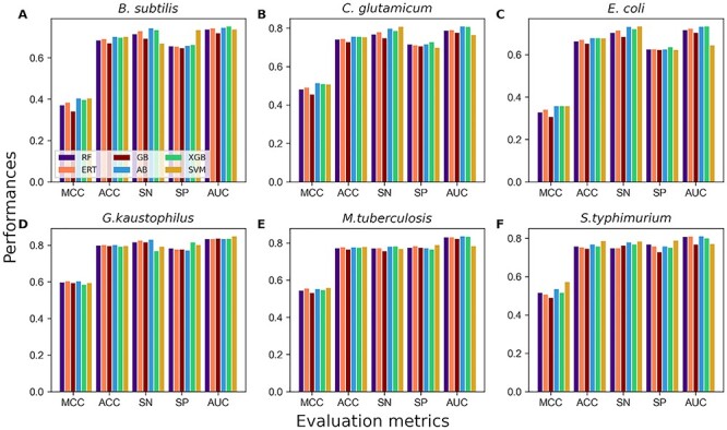
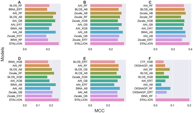
Figure 2.

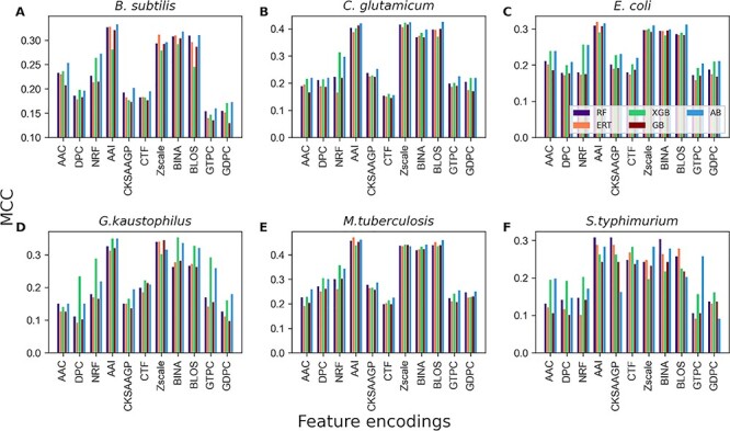
Performances of five different ML classifiers in distinguishing between Kace and non-Kace with respect to 11 feature descriptors. (A) B. subtilis (B) C. glutamicum, (C) E. coli, (D) G. kaustophilus, (E) M. tuberculosis and (F) S. typhimurium.

Figure 1.

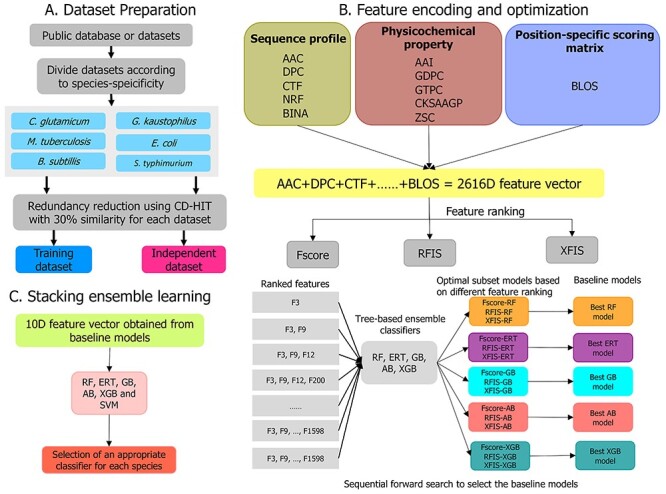
An overview of the STALLION framework for predicting prokaryotic lysine acetylation sites. Schematic display of the three stages in the construction of STALLION is shown.

Feature representation

The sequences in the training dataset of each species are encoded based on AAI (525D), AAC (21D), DPC (441D), CKSAAGP (150D), CTF (343D), Zscale (105D), BINA (441D), BLOS (420D), GTPC (125D), GDPC (25D) and NRF (20D) encoding schemes. We linearly integrated these 11 encodings for each sequence and obtained a 2616D feature vector. Thus, the training dataset of B. subtilis, C. glutamicum, E. coli, G. kaustophilus, M. tuberculosis, and S. typhimurium are represented as a 3142 × 2616, 2104 × 2616, 13,184 × 2616, 412 × 2616, 1730 × 2616 and 396 × 2616 matrix, respectively.

Feature optimization and selection

Each sequence contains a high-dimensional feature vector (2616D) that may include irrelevant or redundant information. Consequently, the predictive performance decreased and required vast computational resources during model training [80, 78]. We employed a two-step feature selection strategy to select the most informative features from the original feature dimension [80]. In the first step, each feature gets a score based on the scoring functions. Here, we employed three different scoring functions, viz. F-score, feature importance score (FIS) estimated by RF (RFIS) and FIS calculated by XGB (XFIS) according to their ability to distinguish Kace sites from non-Kace sites. Thereafter, we sorted the original feature dimension in descending order based on their scores. In total, we generated three feature lists (F-score, RFIS and XFIS), where F-score and RFIS contained the top 2000 features and XFIS included features that have only non-zero value (~500 features).

Second, a sequential forward search (SFS) was applied independently on three feature lists to identify suboptimum feature subsets. Letter r and s denoted the ranked feature list and suboptimum subset, respectively. In SFS, k (k = 5 for F-score and RFIS; k = 2 for XFIS) moved most informative features from r to s, which was inputted into five different classifiers independently and the performance evaluated by employing a 5-fold cross-validation in s. This process was repeated until r became empty. Ultimately, the feature subset for each classifier that achieved superior performance in terms of Mathews correlation coefficient (MCC) was considered an optimal set for each species. Generally, one of the scoring functions and a classifier was to be used to determine the optimal feature set [48, 76]. However, we applied a systematic approach for identifying the optimal feature set, although this procedure is computationally extensive. As we used three different ranked lists and five different classifiers, we obtained 15 models for each species.

Stacking ensemble learning

For each classifier, we selected the best model from three different suboptimum subset models. Consequently, we obtained five optimal baseline models for each species. Predicted probabilities and class labels received from baseline models were combined and considered as a new feature vector (10D). In general, the product of baseline models was trained with logistic regression while developing the final prediction model [48, 75]. However, we explored six classifiers that included the five tree-based classifiers and SVM. The reason for including SVM is that the new feature vector was in the range of 0–1 and can be handled well by SVM. All these classifiers were trained using ten randomized 5-fold cross-validation procedures. Given that MCC is our objective function during 5-fold cross-validation, it might be possible to overfit the prediction model to attain the highest MCC. Therefore, we repeated 5-fold cross-validation procedures ten times by randomly partitioning the training dataset, leading to 10 optimal feature sets for each classifier. For instance, SVM of C and parameters have ten values each. However, we selected the median parameters of C and for developing the final prediction model. Such randomized cross-validation techniques can avoid overfitting [47]. Finally, the average performances obtained from the randomized 5-fold cross-validations were compared for selecting the best model for each species.

Additional feature encoding

We also tested K-nearest neighbor (KNN) encoding in this study, which is not part of STALLION. KNN encoding makes features for a given sequence based on the similarity of that sequence to the n samples from the training dataset (KAce and non-KAce). In particular, for a given two sequences R₁ and R₂ with the fixed length, the similarity score F(R₁, R₂) is computed as follows:

(1)

where and represent amino acid residues of two sequences at the jth position, and K is the sequence length. For two amino acids m and n, the similarity score is defined as follows:

(2)

where (m, n) similarity score for two amino acids derived from the BLOSUM 62 substitution matrix [81], A is the substitution matrix and min(A)/max(A) represents the smallest/largest value in the matrix, respectively. In this study, we set X = 2, 4, 8, 16, 32, 64 and 128 to generate a 7D feature vector for a given sequence.

Implementation

All cross-validations and independent evaluations were executed in a server with CentOS Linux 7.6 and Python 2.7.5. Notably, all ML classifiers (RF, ERT, GB, ERT and XGB v0.82; https://pypi.org/project/xgboost/) were built and optimized by Scikit-learn v0.18.1 package [82]. We computed three different (F-score, RFIS and XFIS) scoring functions to rank the features using the same package. In addition, feature encodings employed in this study were computed using our in-house code. Notably, a few open-source packages such as iLearn [56] and iFeature [57] can compute most feature encodings employed here.

Performance evaluation strategies

Six performance measurements were applied to evaluate the model performance as widely employed in other studies [83, 84], including MCC, sensitivity (Sn), specificity (Sp), accuracy (ACC), balanced accuracy (BACC) and area under the receiver operating characteristics (ROC) curve (AUC). The definition of the metrics is as follows:

(3)

where TP, TN, FP and FN, respectively denote true positives, true negatives, false positives and false negatives. Furthermore, ROC curves and AUC values were used to assess overall performance.

Results and discussion

Performance evaluation between different feature encoding methods and classifiers

We systematically investigated the effect of various feature encodings and classifiers in prokaryotic Kace site predictions by employing five tree-based ensemble classifiers (RF, GB, ERT, XGB and AB) and eleven feature encodings including sequence-based, physicochemical properties and position-specific scoring matrix. We performed a ten times randomized 5-fold cross-validation test for constructing each model for each species dataset and compared the performances among 55 models (11 encodings × 5 classifiers). Figure 2 shows that four encodings (AAI, Zscale, BINA and BLOS) achieved similar performances and were significantly better than the other seven encodings for most prokaryotic species (B. subtilis, C. glutamicum, E. coli, G. kaustophilus and M. tuberculosis). However, we noted that six encodings achieved similar performances and were significantly higher than the other five encodings (AAC, DPC, NRF, GTPC and GDPC) for S. typhimurium. Overall, four encodings (AAI, Zscale, BINA and BLOS) were found to be superior compared to their counterparts. Nevertheless, other encodings also possessed essential information to support Kace site prediction. To get an overview of the performance of each classifier on Kace prediction, we computed an average performance of 66 models (11 encodings × 6 species) for each classifier. The results showed that AB, XGB, RF, ERT and GB achieved average MCCs of 0.261, 0.255, 0.241, 0.232 and 0.230, respectively. Notably, all classifiers performed reasonably well in Kace site prediction; however, AB was found to be marginally superior. Rather than searching for the best model, integrating the above information and developing a robust model is admissible. In this study, we applied a stacking approach similar to recent studies [76, 85, 86].

Figure 3.

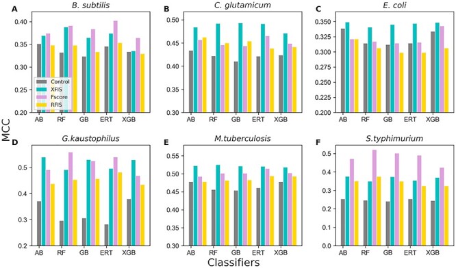
Performance comparisons between the control and the three optimal models for each classifier. Sequential forward search identified the optimal model for each classifier from Fscore, RFIS, and XFIS. (A) B. subtilis (B) C. glutamicum, (C) E. coli, (D) G. kaustophilus, (E) M. tuberculosis and (F) S. typhimurium.

Identification of the optimal model of each classifier for six species

As mentioned in the methods section, we applied three different scoring functions to rank features, each with its own pros and cons. For example, F-score and RFIS assign a relative score for all given features. However, XFIS excludes ~70% of the features and designates a relative score for the remaining features. Supplementary Figure S1 shows the performances of the five classifiers for different feature sets in the C. glutamicum species. Here, we observed that the performance increased steadily, achieved maximum accuracy and subsequently remained in an equilibrium state for most classifiers based on the F-score (Supplementary Figure S1A) and RFIS (Supplementary Figure S1B). However, for XFIS, performance increased slowly until the optimal one and subsequently deteriorated while adding more features (SupplementaryFigure S1C), regardless of the classifiers.

Figure 4.

Performance comparison of six different classifiers for predicting Kace sites during stacking strategy and 10 randomized 5-fold cross-validation. Performances expressed in terms of MCC, ACC, Sn, Sp and AUC. (A) B. subtilis (B) C. glutamicum, (C) E. coli, (D) G. kaustophilus, (E) M. tuberculosis and (F) S. typhimurium.

The size of the optimal feature set varied among five classifiers for each one of the three different approaches (F-score, RFIS and XFIS). For example, RF, ERT, GB, XGB and AB possessed 1000, 520, 790, 260 and 410 optimal feature sets, respectively, from F-score identified by SFS. The corresponding classifiers had 140, 1290, 211, 120 and 150D optimal feature sets from RFIS and 30, 38, 31, 52 and 44D optimal feature sets from XFIS. Similarly, the best model for each classifier from three different approaches showed different sizes of optimal feature sets. For example, RF possessed three models with 1000, 140 and 40D optimal feature sets. However, we selected the best model based on maximal accuracy. The same procedure was followed for the other species and the best three models were selected for each classifier, whose performances were compared with the control.

Figure 3 shows that the performances of the optimal model were consistently better than the control, thus indicating the necessity of feature selection techniques to exclude irrelevant information from the original dimension. For three species (C. glutamicum, E. coli and M. tuberculosis), the optimal feature sets obtained from XFIS achieved superior performances for five classifiers compared to their counterparts (F-score and RFIS). In two species (S. typhimurium and B. subtilis), the optimal feature set extracted from F-score achieved excellent performances for five classifiers compared to their counterparts (XFIS and RFIS). However, for G. kaustophilus, the optimal feature sets derived from the F-score showed improved performance for RF and ERT classifiers. The remaining three classifiers showed improved performance upon the acquisition of optimal features from XFIS. Unexpectedly, the optimal feature set derived from RFIS did not show the best performance. Notably, the best models for five classifiers have been considered as baseline models in each species and utilized for subsequent analysis. Overall, our systematic feature selection analysis suggests that it is essential to apply different scoring functions to rank features and employ different classifiers individually for SFS to obtain their corresponding optimal feature set.

Figure 5.

Performance comparison between STALLION and single feature-based models in classifying Kace from non-Kace sites during cross-validation. (A) B. subtilis (B) C. glutamicum, (C) E. coli, (D) G. kaustophilus, (E) M. tuberculosis and (F) S. typhimurium.

Construction of STALLION

Stacking is an ensemble technique that considers different predictive models to generate a stable stacked model. This approach employs an efficient scheme to decrease the generalization error rate of various predictive models [87–89]. The predicted values (predicted probability of Kace and class label) from the five baseline models were combined to generate a 10D feature vector. Unlike previous approaches [44, 76], we systematically evaluated six different classifiers by training with a new 10D feature vector using 10 randomized 5-fold cross-validations (Figure 4). The results showed that the five classifiers (RF, ERT, AB, XGB and SVM) achieved similar performances, which were marginally better than GB. Among these five classifiers, we selected the AB classifier for three species (B. subtilis, C. glutamicum and G. kaustophilus), the SVM classifier for two species (M. tuberculosis and S. typhimurium), and the XGB classifier for E. coli, whose performances are marginally superior to its counterparts. Six species models were commonly named as STALLION that achieved ACC, MCC and AUC of 0.403, 0.700 and 0.745, respectively for B. subtilis; 0.513, 0.756 and 0.809, respectively for C. glutamicum; 0.357, 0.678 and 0.733, respectively for E. coli; 0.603, 0.801 and 0.836, respectively for G. kaustophilus; 0.557, 0.779 and 0.782, respectively for M. tuberculosis; and 0.571, 0.785 and 0.770, respectively for S. typhimurium.

Figure 6.

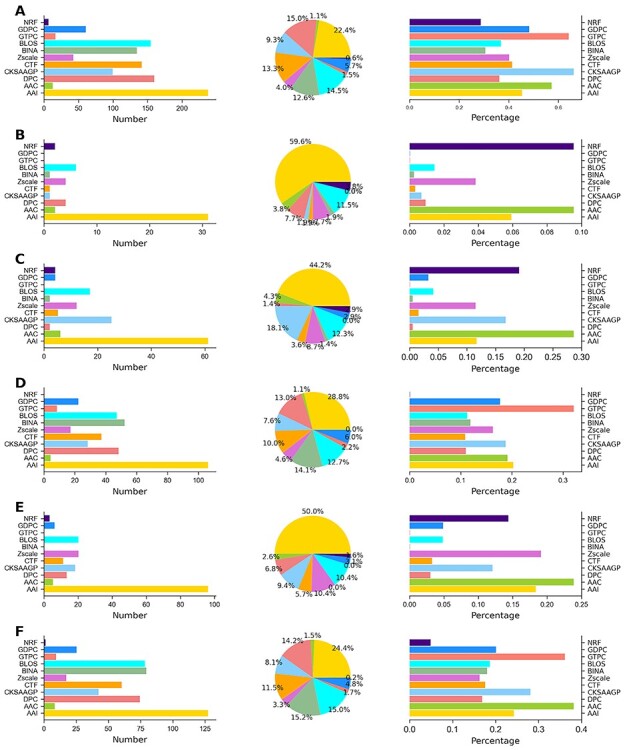
Distribution analysis of generated optimal feature sets across the six species. Panels (A)–(F) illustrate distributions of feature types included in optimal feature sets for B. subtilis, C. glutamicum, E. coli, G. kaustophilus, M. tuberculosis and S. typhimurium, respectively. Each panel containing three figures represent number of each feature type selected in the optimal feature set, portion of the types of features selected in the optimal feature set, and percentage of each feature type selected in the optimal feature set.

Comparison of STALLION with single feature-based models

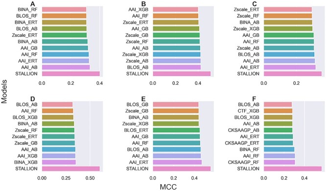
To show the advantage of our proposed stacked approach, we compared STALLION with the single feature-based models. We selected the top 10 single feature-based models from Figure 2 and compared them with STALLION for six species. Figure 5 shows that STALLION significantly outperformed single feature-based models for all six species, whose MCC was 6.9–9.4% higher for B. subtilis, 8.8–11.1% higher for C. glutamicum, 3.7–6.1% higher for E. coli, 24.9–28.2% higher for G. kaustophilus, 8.6–11.7% higher for M. tuberculosis and 26.2–29.3% higher for S. typhimurium. The superior performance of STALLION over the single feature-based models was primarily due to the novelty introduced in our approach, which included (i) feature fusion strategy, (ii) selecting the optimal feature set from hybrid features for each classifier independently and their respective baseline model construction and (iii) selecting an appropriate classifier for stacking model construction.

Figure 7.

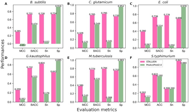
Performance comparison between STALLION and ProAcePred2.0 in classifying Kace from non-Kace sites during independent test. (A) B. subtilis (B) C. glutamicum, (C) E. coli, (D) G. kaustophilus, (E) M. tuberculosis and (F) S. typhimurium.

Feature contribution analysis

To understand the contribution of different features in the optimal feature set for each species, we analyzed their composition and distribution. It is worth mentioning that five classifier models have different optimal feature subsets for each species. Instead of focusing on each subset, we considered the maximum size of the optimal feature subset that potentially includes the other four subsets for five species (B. subtilis, C. glutamicum, E. coli, M. tuberculosis and S. typhimurium). For example, in C. glutamicum, RF, ERT, GB, XGB and AB contained 30, 38, 31, 52 and 44D optimal feature subsets, respectively. Here, 52D had other feature subsets. However, in G. kaustophilus, different optimal subsets were combined to investigate their role.

Figure 6 indicates that the feature distribution in the optimal feature set among six species showed significant differences; however, some subtle similarities were noted. Particularly, AAI contributed 22.4%, 59.6%, 44.2%, 28.8%, 50.0% and 24.4% of the total optimal features for B. subtilis, C. glutamicum, E. coli, G. kaustophilus, M. tuberculosis and S. typhimurium, respectively. This result implies that the AAI feature contribution is important for six species, suggesting their critical importance in Kace prediction. Six encodings (AAC, DPC, CKSAAGP, CTF, Zscale and BLOS) consistently contributed to the optimal feature set for all species. Still, the contribution level varied among them suggesting a supporting role played in Kace prediction. Furthermore, we observed that GTPC and GDPC, GTPC, NRF and GTPC and BINA did not contribute to the final prediction for C. glutamicum, E. coli, G. kaustophilus and M. tuberculosis, respectively. Overall, apart from AAI, the rest of the feature contribution varied considerably among species, thus suggesting that Kace sites in these species might have different characteristics.

Figure 8.

Performance comparison between STALLION and single feature-based models in classifying Kace from non-Kace sites during independent test. (A) B. subtilis (B) C. glutamicum, (C) E. coli, (D) G. kaustophilus, (E) M. tuberculosis and (F) S. typhimurium.

Performance validation using the independent test

We further evaluated STALLION using independent datasets and compared their performances with the existing method. Since 2009, several computational tools have been reported for Kace site prediction. Notably, Chen et al. [37] recently evaluated species-specific ProAcePred 2.0 predictor using an independent dataset and compared the performance with existing methods, including species-specific ProAcePred, general predictors viz. EnsemblePail, PSKAcePred, Phosida and PLMLA. The result showed that ProAcePred 2.0 significantly outperformed generic predictors and their previous version ProAcePred. Therefore, only ProAcePred 2.0 was considered in this study for comparison and other methods were excluded for the following reasons: (i) comparing species-specific predictor with a generic predictor is unfair, which is evident from previous studies [36, 37] and (ii) ProAcePred 2.0 is the upgraded version of ProAcePred.

It is worth mentioning that the independent dataset for each species was submitted to the ProAcePred 2.0 web server (http://computbiol.ncu.edu.cn/PAPred) and the predictions were computed based on the given default threshold. Notably, the ProAcePred 2.0 returns Kace site and its predicted probability value, but not non-Kace predicted probability values. Therefore, it might be unfeasible to compute the AUC value with partial probability information. However, we compared the performances between two methods in terms of MCC, which is an intuitive and straightforward metric while dealing with an imbalanced dataset, as mentioned in [90]. Our evaluation results showed that STALLION achieved MCC of 0.295, 0.329, 0.390, 0.259, 0.380 and 0.202 for B. subtilis, C. glutamicum, E. coli, G. kaustophilus, M. tuberculosis and S. typhimurium, respectively (Figure 7 and Supplementary Table S2). STALLION outperformed ProAcePred 2.0 by >20.0% in MCC value for five species (B. subtilis, C. glutamicum, E. coli, G. kaustophilus and M. tuberculosis) and 9.1% in MCC value for S. typhimurium. STALLION provided better performance than ProAcePred2.0 because of the following: (i) Unlike ProAcePred 2.0, we excluded KNN feature encoding from the stacking framework based on our systematic analysis that identified the overfitting nature of KNN encoding during cross-validation (see section below); (ii) Unlike ProAcePred 2.0 simple feature selection approach, we employed a rigorous process by utilizing three different scoring functions and SFS to identify the optimal feature set independently for each classifier, which is time-consuming and (iii) Unlike a single model in ProAcePred 2.0, our stacking strategy integrates five tree-based ensemble baseline models leading to more accurate Kace site predictions.

Like STALLION and the best single feature-based models’ cross-validation performance comparison, we carried out independent tests. Figure 8 shows that STALLION outperformed single feature-based models for all six species, whose MCC was 2.39–10.68% higher for B. subtilis, 1.18–6.08% higher for C. glutamicum, 4.0–9.5% higher for E. coli, 2.5–8.7% higher for G. Kaustophilus, 3.51–10.89% higher for M. tuberculosis and 11.29–19.54% higher for S. typhimurium. These results yet again highlight the significance of our systematic approach in model construction.

Overfitting nature of KNN encoding in Kace prediction

KNN feature encoding is widely applied for the identification of PTM sites, including previous Kace site prediction methods [36, 37]. Similar to previous studies, we also incorporated it into 11 encodings in the stacking framework. The preliminary result showed that all species models’ prediction performance significantly improved compared with the STALLION during cross-validation. However, the corresponding model performance with independent datasets was slightly better than the random prediction and considerably lower than the STALLION. Hence, we excluded KNN encoding from the stacking framework (STALLION). To better understand the phenomenon, we developed KNN-based five tree-based models for each species and examined their cross-validation and independent validation performances (Table 2). The results showed that four (RF, ERT, AB and XGB) out of five classifiers achieved similar performances, which were marginally better than GB with average AUCs of 0.895, 0.901, 0.888, 0.888, 0.895 and 0.872 for five models, namely B. subtilis, C. glutamicum, E. coli, G. kaustophilus, M. tuberculosis and S. typhimurium, respectively. The corresponding metrics on independent tests were 0.602, 0.665, 0.621, 0.597, 0.670 and 0.619 for the six species. The performance gap (difference in AUC) between the training and independent datasets in all six species significantly increased from 22.46 to 29.32%, clearly indicating the overestimation of KNN encoding during training regardless of the classifiers. Owing to the over-fitting nature of the KNN encoding scheme, we highly recommend testing KNN encoding transferability before incorporating it into any computational frameworks requiring huge computations.

Table 2.

Performance comparison of various classifiers on KNN encoding during training and independent tests

Species	Classifier	MCC	ACC	Sn	Sp	AUC	MCC	ACC	Sn	Sp	AUC
B. subtillis	RF	0.599	0.799	0.757	0.840	0.907	0.105	0.573	0.608	0.569	0.630
	ERT	0.605	0.802	0.833	0.771	0.903	0.106	0.568	0.616	0.563	0.612
	GB	0.583	0.791	0.778	0.805	0.857	0.108	0.558	0.632	0.550	0.562
	AB	0.623	0.805	0.701	0.908	0.908	0.106	0.650	0.504	0.666	0.623
	XGB	0.652	0.799	0.597	1.000	0.899	0.070	0.702	0.368	0.737	0.581
C. glutamicum	RF	0.616	0.808	0.816	0.800	0.915	0.168	0.610	0.687	0.602	0.690
	ERT	0.599	0.799	0.786	0.813	0.917	0.168	0.610	0.687	0.602	0.676
	GB	0.590	0.795	0.806	0.784	0.828	0.124	0.590	0.627	0.587	0.608
	AB	0.646	0.823	0.844	0.801	0.922	0.203	0.607	0.759	0.592	0.678
	XGB	0.648	0.821	0.886	0.757	0.923	0.196	0.578	0.783	0.558	0.673
E. coli	RF	0.582	0.791	0.776	0.806	0.905	0.152	0.559	0.654	0.534	0.631
	ERT	0.578	0.789	0.806	0.772	0.905	0.151	0.559	0.651	0.535	0.624
	GB	0.576	0.788	0.780	0.797	0.824	0.131	0.543	0.645	0.517	0.582
	AB	0.610	0.804	0.755	0.852	0.909	0.241	0.622	0.693	0.604	0.657
	XGB	0.627	0.782	0.565	1.000	0.895	0.146	0.675	0.424	0.741	0.610
G. kaustophilus	RF	0.612	0.806	0.796	0.816	0.908	0.104	0.502	0.706	0.484	0.630
	ERT	0.631	0.816	0.811	0.820	0.912	0.061	0.479	0.647	0.464	0.625
	GB	0.626	0.813	0.801	0.825	0.835	0.058	0.474	0.647	0.458	0.582
	AB	0.646	0.823	0.816	0.830	0.866	0.011	0.445	0.588	0.432	0.555
	XGB	0.631	0.816	0.820	0.811	0.919	0.072	0.498	0.647	0.484	0.593
M. tuberculosis	RF	0.663	0.831	0.820	0.843	0.928	0.241	0.646	0.735	0.634	0.681
	ERT	0.652	0.826	0.836	0.816	0.917	0.237	0.641	0.735	0.628	0.666
	GB	0.636	0.818	0.809	0.827	0.853	0.206	0.612	0.721	0.597	0.667
	AB	0.685	0.842	0.806	0.878	0.932	0.234	0.656	0.706	0.650	0.689
	XGB	0.694	0.845	0.791	0.899	0.845	0.197	0.651	0.647	0.652	0.649
S. typhimurium	RF	0.540	0.770	0.768	0.773	0.893	0.096	0.542	0.700	0.535	0.615
	ERT	0.551	0.775	0.783	0.768	0.843	0.106	0.564	0.700	0.558	0.645
	GB	0.551	0.775	0.768	0.783	0.813	0.095	0.537	0.700	0.530	0.615
	AB	0.591	0.796	0.788	0.803	0.906	0.048	0.520	0.600	0.516	0.619
	XGB	0.602	0.801	0.823	0.778	0.907	0.003	0.507	0.500	0.507	0.603

Note: The first and the second columns represent the species and the ML classifiers. Columns 3–7 represent MCC, ACC, Sn, Sp and AUC of the ML classifier performance on the training dataset. Columns 8–12 represent MCC, ACC, Sn, Sp and AUC of the ML classifier performance on the independent dataset.

Availability of online webserver

Publicly accessible web servers can help experimental or biomedical researchers to identify the putative functional sites, which will aid further experimental characterization. To help the user identify high-throughput putative Kace sites from six prokaryotic species, we implemented the STALLION web server, which is freely accessible at: http://thegleelab.org/STALLION. The STALLION web server is maintained by an Apache HTTP server and configured in a 16-core CentOs Linux 7.6 server machine with 64GB RAM and a 2 TB hard disk. We have given the detailed instructions for using the STALLION in the following link: http://thegleelab.org/STALLION/Staltutorial.html. In addition, we provided the server running time of our independent datasets in the above link.

Conclusions

This study presented STALLION, a stacking framework for the accurate Kace site prediction from six different prokaryotic species. STALLION employed 11 distinct feature encoding schemes (categorized into three groups) to encode protein fragments. Subsequently, a rigorous feature selection approach was employed to carefully select the optimal feature set for each of the five different tree-based ensemble algorithms and constructed their respective baseline models for each species. Finally, the predicted output was derived from five baseline models which were trained with an appropriate classifier to build the stable, stacked STALLION models. Our proposed method STALLION outperformed the current state-of-the-art predictor for identifying Kace sites on the independent data sets across six different species. It is expected that STALLION methodology and a user-friendly web server based on the stacked model for six prokaryotic species will expedite the discovery of putative Kace sites and greatly assist the effort of a broader research community for functional characterization. Our study identified that heterogeneous and complementary features derived from different perspectives helped to improve predictor performance. We will continually attempt to investigate other informative features, examine their contribution and refine our prediction platform.

Overall, the STALLION method has achieved a robust performance in Kace site prediction, whose prediction performance requires further improvement in several aspects. Novel computational frameworks have been reported recently, including a DL-based hybrid framework [86] and DL-based approaches with automatically generated features [91, 92]. In future, we will examine the possibility of these approaches and select the appropriate one to further improve prediction performance of Kace sites.

Key Points

• We propose a stacking framework STALLION and implement it as a user-friendly webserver for accurate identification of prokaryotic Kace sites.

• STALLION utilized 11 different features encoding schemes and combined five tree-based ensemble algorithms to build stable stacked models.

• Extensive benchmarking experiments demonstrated that STALLION outperformed its constituent baseline models in both training and independent datasets, thus highlighting its excellent generalization capability.

Shaherin Basith is a research assistant professor in the Department of Physiology, Ajou University School of Medicine, Republic of Korea. Her main area of research is exploring the structure–function relationships of proteins using state-of-the-art molecular modeling tools, phylogenetic analysis and biomolecular simulations. She is also actively involved in the application of machine learning tools for peptide and small molecule drug discovery.

Gwang Lee is a professor in the Department of Physiology, Ajou University School of Medicine, Republic of Korea. His main research interests include the integration of triple omics (transcriptomics, metabolomics and proteomics) for nanotoxicity studies, machine learning, neurodegenerative diseases and biomolecular simulations targeting therapeutically important proteins or enzymes.

Balachandran Manavalan is an assistant professor in the Department of Physiology, Ajou University School of Medicine, Republic of Korea. He is also an associate member of Korea Institute for Advanced Study, Republic of Korea. His research interests include artificial intelligence, bioinformatics, machine learning, big data and functional genomics.

Funding

This work was fully supported by the National Research Foundation of Korea (NRF) funded by the Korean government (MSIT) (2021R1A2C1014338, 2019R1I1A1A01062260 and 2020R1A4A4079722).

Data availability

Training and independent datasets used in this study could be freely downloaded by clicking the below link: http://thegleelab.org/STALLION/StalData.html

References

- 1. Crick F. Central dogma of molecular biology. Nature 1970;227:561–3. [DOI] [PubMed] [Google Scholar]
- 2. Soffer RL. Post-translational modification of proteins catalyzed by aminoacyl-tRNA-protein transferases. Mol Cell Biochem 1973;2:3–14. [DOI] [PubMed] [Google Scholar]
- 3. Wold F. In vivo chemical modification of proteins (post-translational modification). Annu Rev Biochem 1981;50:783–814. [DOI] [PubMed] [Google Scholar]
- 4. Krishna RG, Wold F. Post-translational modification of proteins. Adv Enzymol Relat Areas Mol Biol 1993;67:265–98. [DOI] [PubMed] [Google Scholar]
- 5. Rogers LD, Overall CM. Proteolytic post-translational modification of proteins: proteomic tools and methodology. Mol Cell Proteomics 2013;12:3532–42. [DOI] [PMC free article] [PubMed] [Google Scholar]
- 6. Wang ZA, Cole PA. The chemical biology of reversible lysine post-translational modifications. Cell Chem Biol 2020;27:953–69. [DOI] [PMC free article] [PubMed] [Google Scholar]
- 7. Karve TM, Cheema AK. Small changes huge impact: the role of protein posttranslational modifications in cellular homeostasis and disease. J Amino Acids 2011;2011:207691. [DOI] [PMC free article] [PubMed] [Google Scholar]
- 8. Ramazi S, Zahiri J. Posttranslational Modifications in Proteins: Resources, Tools and Prediction Methods, Database (Oxford) 2021, Oxford: Oxford University Press, 2021. [DOI] [PMC free article] [PubMed]
- 9. Lee TY, Huang HD, Hung JH, et al. dbPTM: an information repository of protein post-translational modification. Nucl Acids Res 2006;34:D622–7. [DOI] [PMC free article] [PubMed] [Google Scholar]
- 10. Sun X, Li Z, Liu H, et al. Large-scale identification of lysine acetylated proteins in vegetative hyphae of the rice blast fungus. Sci Rep 2017;7:15316. [DOI] [PMC free article] [PubMed] [Google Scholar]
- 11. Drazic A, Myklebust LM, Ree R, et al. The world of protein acetylation. Biochim Biophys Acta 1864;2016:1372–401. [DOI] [PubMed] [Google Scholar]
- 12. Xia C, Tao Y, Li M, et al. Protein acetylation and deacetylation: an important regulatory modification in gene transcription (review). Exp Ther Med 2020;20:2923–40. [DOI] [PMC free article] [PubMed] [Google Scholar]
- 13. Polevoda B, Sherman F. Nalpha -terminal acetylation of eukaryotic proteins. J Biol Chem 2000;275:36479–82. [DOI] [PubMed] [Google Scholar]
- 14. Christensen DG, Xie X, Basisty N, et al. Post-translational protein acetylation: an elegant mechanism for bacteria to dynamically regulate metabolic functions. Front Microbiol 2019;10:1604. [DOI] [PMC free article] [PubMed] [Google Scholar]
- 15. Fraga MF, Ballestar E, Villar-Garea A, et al. Loss of acetylation at Lys16 and trimethylation at Lys20 of histone H4 is a common hallmark of human cancer. Nat Genet 2005;37:391–400. [DOI] [PubMed] [Google Scholar]
- 16. Kim D, Nguyen MD, Dobbin MM, et al. SIRT1 deacetylase protects against neurodegeneration in models for Alzheimer's disease and amyotrophic lateral sclerosis. EMBO J 2007;26:3169–79. [DOI] [PMC free article] [PubMed] [Google Scholar]
- 17. Medzihradszky KF. Peptide sequence analysis. Methods Enzymol 2005;402:209–44. [DOI] [PubMed] [Google Scholar]
- 18. Deng W, Wang C, Zhang Y, et al. GPS-PAIL: prediction of lysine acetyltransferase-specific modification sites from protein sequences. Sci Rep 2016;6:39787. [DOI] [PMC free article] [PubMed] [Google Scholar]
- 19. Yu K, Zhang Q, Liu Z, et al. Deep learning based prediction of reversible HAT/HDAC-specific lysine acetylation. Brief Bioinform 2020;21:1798–805. [DOI] [PubMed] [Google Scholar]
- 20. Yang Y, Wang H, Li W, et al. Prediction and analysis of multiple protein lysine modified sites based on conditional wasserstein generative adversarial networks. BMC Bioinform 2021;22:171. [DOI] [PMC free article] [PubMed] [Google Scholar]
- 21. Xiu Q, Li, D, Li, H, Wang, Net al. Prediction method for lysine acetylation sites based on LSTM network. In: 2019 IEEE 7th International Conference on Computer Science and Network Technology (ICCSNT). Manhattan: IEEE, 2019, p. 179–82.
- 22.Basith S, Chang H J, Nithiyanandam S, Shin T H, Manavalan B, Lee G. Recent trends on the development of machine learning approaches for the prediction of lysine acetylation sites, Curr Med Chem. 2021. doi: 10.2174/0929867328999210902125308. [DOI] [PubMed] [Google Scholar]
- 23. Li A, Xue Y, Jin C, et al. Prediction of Nepsilon-acetylation on internal lysines implemented in Bayesian discriminant method. Biochem Biophys Res Commun 2006;350:818–24. [DOI] [PMC free article] [PubMed] [Google Scholar]
- 24. Li S, Li H, Li M, et al. Improved prediction of lysine acetylation by support vector machines. Protein Pept Lett 2009;16:977–83. [DOI] [PubMed] [Google Scholar]
- 25. Xu Y, Wang XB, Ding J, et al. Lysine acetylation sites prediction using an ensemble of support vector machine classifiers. J Theor Biol 2010;264:130–5. [DOI] [PubMed] [Google Scholar]
- 26. Lee TY, Hsu JB, Lin FM, et al. N-Ace: using solvent accessibility and physicochemical properties to identify protein N-acetylation sites. J Comput Chem 2010;31:2759–71. [DOI] [PubMed] [Google Scholar]
- 27. Shao J, Xu D, Hu L, et al. Systematic analysis of human lysine acetylation proteins and accurate prediction of human lysine acetylation through bi-relative adapted binomial score Bayes feature representation. Mol Biosyst 2012;8:2964–73. [DOI] [PubMed] [Google Scholar]
- 28. Shi SP, Qiu JD, Sun XY, et al. PLMLA: prediction of lysine methylation and lysine acetylation by combining multiple features. Mol Biosyst 2012;8:1520–7. [DOI] [PubMed] [Google Scholar]
- 29. Suo SB, Qiu JD, Shi SP, et al. Position-specific analysis and prediction for protein lysine acetylation based on multiple features. PLoS One 2012;7:e49108. [DOI] [PMC free article] [PubMed] [Google Scholar]
- 30. Suo SB, Qiu JD, Shi SP, et al. Proteome-wide analysis of amino acid variations that influence protein lysine acetylation. J Proteome Res 2013;12:949–58. [DOI] [PubMed] [Google Scholar]
- 31. Hou T, Zheng G, Zhang P, et al. LAceP: lysine acetylation site prediction using logistic regression classifiers. PLoS One 2014;9:e89575. [DOI] [PMC free article] [PubMed] [Google Scholar]
- 32. Lu CT, Lee TY, Chen YJ, et al. An intelligent system for identifying acetylated lysine on histones and nonhistone proteins. Biomed Res Int 2014;2014:528650. [DOI] [PMC free article] [PubMed] [Google Scholar]
- 33. Li Y, Wang M, Wang H, et al. Accurate in silico identification of species-specific acetylation sites by integrating protein sequence-derived and functional features. Sci Rep 2014;4:5765. [DOI] [PMC free article] [PubMed] [Google Scholar]
- 34. Qiu WR, Sun BQ, Xiao X, et al. iPTM-mLys: identifying multiple lysine PTM sites and their different types. Bioinformatics 2016;32:3116–23. [DOI] [PubMed] [Google Scholar]
- 35. Wuyun Q, Zheng W, Zhang Y, et al. Improved species-specific lysine acetylation site prediction based on a large variety of features set. PLoS One 2016;11:e0155370. [DOI] [PMC free article] [PubMed] [Google Scholar]
- 36. Chen G, Cao M, Luo K, et al. ProAcePred: prokaryote lysine acetylation sites prediction based on elastic net feature optimization. Bioinformatics 2018;34:3999–4006. [DOI] [PubMed] [Google Scholar]
- 37. Chen G, Cao M, Yu J, et al. Prediction and functional analysis of prokaryote lysine acetylation site by incorporating six types of features into Chou's general PseAAC. J Theor Biol 2019;461:92–101. [DOI] [PubMed] [Google Scholar]
- 38. Ning Q, Yu M, Ji J, et al. Analysis and prediction of human acetylation using a cascade classifier based on support vector machine. BMC Bioinform 2019;20:346. [DOI] [PMC free article] [PubMed] [Google Scholar]
- 39. Yu B, Yu Z, Chen C, et al. DNNAce: prediction of prokaryote lysine acetylation sites through deep neural networks with multi-information fusion. Chemom Intel Lab Syst 2020;103999. [Google Scholar]
- 40. LeCun Y, Bengio Y, Hinton G. Deep learning. Nature 2015;521:436–44. [DOI] [PubMed] [Google Scholar]
- 41. Emmert-Streib F, Yang Z, Feng H, et al. An introductory review of deep learning for prediction models with big data. Front Artif Intell 2020;3:4. [DOI] [PMC free article] [PubMed] [Google Scholar]
- 42. Wei L, Su R, Luan S, et al. Iterative feature representations improve N4-methylcytosine site prediction. Bioinformatics 2019;35:4930–7. [DOI] [PubMed] [Google Scholar]
- 43. Wei L, He W, Malik A, et al. Computational prediction and interpretation of cell-specific replication origin sites from multiple eukaryotes by exploiting stacking framework. Brief Bioinform 2021;22. [DOI] [PubMed] [Google Scholar]
- 44. Charoenkwan P, Chiangjong W, Nantasenamat C, et al. StackIL6: a stacking ensemble model for improving the prediction of IL-6 inducing peptides. Brief Bioinform 2021. [DOI] [PubMed] [Google Scholar]
- 45. Xu H, Zhou J, Lin S, et al. PLMD: an updated data resource of protein lysine modifications. J Genet Genomics 2017;44:243–50. [DOI] [PubMed] [Google Scholar]
- 46. Fu L, Niu B, Zhu Z, et al. CD-HIT: accelerated for clustering the next-generation sequencing data. Bioinformatics 2012;28:3150–2. [DOI] [PMC free article] [PubMed] [Google Scholar]
- 47. Wang J, Li J, Yang B, et al. Bastion3: a two-layer ensemble predictor of type III secreted effectors. Bioinformatics 2019;35:2017–28. [DOI] [PMC free article] [PubMed] [Google Scholar]
- 48. Zhang Y, Xie R, Wang J, et al. Computational analysis and prediction of lysine malonylation sites by exploiting informative features in an integrative machine-learning framework. Brief Bioinform 2019;20:2185–99. [DOI] [PMC free article] [PubMed] [Google Scholar]
- 49. Nilamyani AN, Auliah FN, Moni MA, et al. PredNTS: improved and robust prediction of nitrotyrosine sites by integrating multiple sequence features. Int J Mol Sci 2021;22. [DOI] [PMC free article] [PubMed] [Google Scholar]
- 50. Hasan MM, Alam MA, Shoombuatong W, et al. NeuroPred-FRL: an interpretable prediction model for identifying neuropeptide using feature representation learning. Brief Bioinform 2021. [DOI] [PubMed] [Google Scholar]
- 51. Manavalan B, Basith S, Shin TH, et al. mAHTPred: a sequence-based meta-predictor for improving the prediction of anti-hypertensive peptides using effective feature representation. Bioinformatics 2019;35:2757–65. [DOI] [PubMed] [Google Scholar]
- 52. Hasan MM, Manavalan B, Khatun MS, et al. Prediction of S-nitrosylation sites by integrating support vector machines and random forest. Mol Omics 2019;15:451–8. [DOI] [PubMed] [Google Scholar]
- 53. Shen J, Zhang J, Luo X, et al. Predicting protein-protein interactions based only on sequences information. Proc Natl Acad Sci U S A 2007;104:4337–41. [DOI] [PMC free article] [PubMed] [Google Scholar]
- 54. Kawashima S, Pokarowski P, Pokarowska M, et al. AAindex: amino acid index database, progress report 2008. Nucl Acids Res 2008;36:D202–5. [DOI] [PMC free article] [PubMed] [Google Scholar]
- 55. Chen YZ, Wang ZZ, Wang Y, et al. Brief Bioinform nhKcr: a new bioinformatics tool for predicting crotonylation sites on human nonhistone proteins based on deep learning. Brief Bioinform 2021. [DOI] [PMC free article] [PubMed] [Google Scholar]
- 56. Chen Z, Zhao P, Li F, et al. iLearn: an integrated platform and meta-learner for feature engineering, machine-learning analysis and modeling of DNA, RNA and protein sequence data. Brief Bioinform 2020;21:1047–57. [DOI] [PubMed] [Google Scholar]
- 57. Chen Z, Zhao P, Li F, et al. iFeature: a python package and web server for features extraction and selection from protein and peptide sequences. Bioinformatics 2018;34:2499–502. [DOI] [PMC free article] [PubMed] [Google Scholar]
- 58. Chen Z, Chen Y-Z, Wang X-F, et al. Prediction of ubiquitination sites by using the composition of k-spaced amino acid pairs. PLoS One 2011;6:e22930. [DOI] [PMC free article] [PubMed] [Google Scholar]
- 59. Sandberg M, Eriksson L, Jonsson J, et al. New chemical descriptors relevant for the design of biologically active peptides. A multivariate characterization of 87 amino acids. J Med Chem 1998;41:2481–91. [DOI] [PubMed] [Google Scholar]
- 60. Yang JH, Choi HP, Yang A, et al. Post-translational modification networks of contractile and cellular stress response proteins in bladder ischemia. Cell 2021;10. [DOI] [PMC free article] [PubMed] [Google Scholar]
- 61. Wei L, Zhou C, Chen H, et al. ACPred-FL: a sequence-based predictor using effective feature representation to improve the prediction of anti-cancer peptides. Bioinformatics 2018;34:4007–16. [DOI] [PMC free article] [PubMed] [Google Scholar]
- 62. Breiman L. Random forests. Mach Learn 2001;45:5–32. [Google Scholar]
- 63. Chen T, Guestrin C. Xgboost: a scalable tree boosting system. In: Proceedings of the 22nd ACM SIGKdd International Conference on Knowledge Discovery and Data Mining. 2016, p. 785–94.
- 64. Schapire RE. Explaining adaboost. Empirical Inference Berlin, Heidelberg: Springer; 2013;37–52. [Google Scholar]
- 65. Friedman JH. Greedy function approximation: a gradient boosting machine. Ann. Stat 2001;1189–232. [Google Scholar]
- 66. Geurts P, Ernst D, Wehenkel L. Extremely randomized trees. Mach Learn 2006;63:3–42. [Google Scholar]
- 67. Cortes C, Vapnik V. Support-vector networks. Mach Learn 1995;20:273–97. [Google Scholar]
- 68. Tang Q, Nie F, Kang J, et al. mRNALocater: enhance the prediction accuracy of eukaryotic mRNA subcellular localization by using model fusion strategy. Mol Ther 2021;29:2617–23. [DOI] [PMC free article] [PubMed] [Google Scholar]
- 69. Charoenkwan P, Nantasenamat C, Hasan MM, et al. Meta-iPVP: a sequence-based meta-predictor for improving the prediction of phage virion proteins using effective feature representation. J Comput Aided Mol Des 2020;34:1105–16. [DOI] [PubMed] [Google Scholar]
- 70. Chen W, Feng P, Nie F. iATP: a sequence based method for identifying anti-tubercular peptides. Med Chem 2020;16:620–5. [DOI] [PubMed] [Google Scholar]
- 71. Khatun MS, Hasan MM, Shoombuatong W, et al. ProIn-fuse: improved and robust prediction of proinflammatory peptides by fusing of multiple feature representations. J Comput Aided Mol Des 2020;34:1229–36. [DOI] [PubMed] [Google Scholar]
- 72. Liu K, Chen W. iMRM: a platform for simultaneously identifying multiple kinds of RNA modifications. Bioinformatics 2020;36:3336–42. [DOI] [PubMed] [Google Scholar]
- 73. Wang D, Zhang Z, Jiang Y, et al. DM3Loc: multi-label mRNA subcellular localization prediction and analysis based on multi-head self-attention mechanism. Nucleic Acids Res 2021;49:e46. [DOI] [PMC free article] [PubMed] [Google Scholar]
- 74. Zhang D, Xu ZC, Su W, et al. iCarPS: a computational tool for identifying protein carbonylation sites by novel encoded features. Bioinformatics 2021;37:171–7. [DOI] [PubMed] [Google Scholar]
- 75. Hasan MM, Basith S, Khatun MS, et al. Meta-i6mA: an interspecies predictor for identifying DNA N6-methyladenine sites of plant genomes by exploiting informative features in an integrative machine-learning framework. Brief Bioinform 2021;22. [DOI] [PubMed] [Google Scholar]
- 76. Wei L, He W, Malik A, et al. Computational prediction and interpretation of cell-specific replication origin sites from multiple eukaryotes by exploiting stacking framework. Brief Bioinform 2020;22:1–15. [DOI] [PubMed] [Google Scholar]
- 77. Manavalan B, Basith S, Shin TH, et al. Meta-4mCpred: a sequence-based meta-predictor for accurate DNA 4mC site prediction using effective feature representation. Mol Ther Nucleic Acids 2019;16:733–44. [DOI] [PMC free article] [PubMed] [Google Scholar]
- 78. Basith S, Manavalan B, Shin TH, et al. SDM6A: a web-based integrative machine-learning framework for predicting 6mA sites in the Rice genome. Mol Ther Nucl Acids 2019;18:131–41. [DOI] [PMC free article] [PubMed] [Google Scholar]
- 79. Wang J, Li J, Hou Y, et al. Bastion hub: a universal platform for integrating and analyzing substrates secreted by gram-negative bacteria. Nucl Acids Res 2021;49:D651–9. [DOI] [PMC free article] [PubMed] [Google Scholar]
- 80. Ferri FJ, Pudil P, Hatef M, et al. Comparative study of techniques for large-scale feature selection. Machine Intelligence and Pattern Recognition Amsterdam: Elsevier, 1994;16:403–13. [Google Scholar]
- 81. Henikoff S, Henikoff JG. Amino acid substitution matrices from protein blocks. Proc Natl Acad Sci U S A 1992;89:10915–9. [DOI] [PMC free article] [PubMed] [Google Scholar]
- 82. Pedregosa F, Varoquaux G, Gramfort A, et al. Scikit-learn: machine learning in python. J Mach Learn Res 2011;12:2825–30. [Google Scholar]
- 83. Su R, Hu J, Zou Q, et al. Empirical comparison and analysis of web-based cell-penetrating peptide prediction tools. Brief Bioinform 2019. [DOI] [PubMed] [Google Scholar]
- 84. Basith S, Manavalan B, Hwan Shin T, et al. Machine intelligence in peptide therapeutics: a next-generation tool for rapid disease screening. Med Res Rev 2020;40:1276–1314. [DOI] [PubMed] [Google Scholar]
- 85. Li F, Chen J, Ge Z, et al. Computational prediction and interpretation of both general and specific types of promoters in Escherichia coli by exploiting a stacked ensemble-learning framework. Brief Bioinform 2021;22:2126–40. [DOI] [PMC free article] [PubMed] [Google Scholar]
- 86. Xie R, Li J, Wang J, et al. DeepVF: a deep learning-based hybrid framework for identifying virulence factors using the stacking strategy. Brief Bioinform 2021;22. [DOI] [PMC free article] [PubMed] [Google Scholar]
- 87. Liang X, Li F, Chen J, et al. Large-scale comparative review and assessment of computational methods for anti-cancer peptide identification. Brief Bioinform 2021;22. [DOI] [PMC free article] [PubMed] [Google Scholar]
- 88. Li F, Guo X, Jin P, et al. Porpoise: a new approach for accurate prediction of RNA pseudouridine sites. Brief Bioinf 2021. [DOI] [PMC free article] [PubMed] [Google Scholar]
- 89. Džeroski S, Ženko B. Is combining classifiers with stacking better than selecting the best one? Mach Learn 2004;54:255–73. [Google Scholar]
- 90. Chicco D, Jurman G. The advantages of the Matthews correlation coefficient (MCC) over F1 score and accuracy in binary classification evaluation. BMC Genomics 2020;21:6. [DOI] [PMC free article] [PubMed] [Google Scholar]
- 91. Charoenkwan P, Nantasenamat C, Hasan MM, et al. BERT4Bitter: a bidirectional encoder representations from transformers (BERT)-based model for improving the prediction of bitter peptides. Bioinformatics 2021. [DOI] [PubMed] [Google Scholar]
- 92. Lv H, Dao FY, Guan ZX, et al. Deep-Kcr: accurate detection of lysine crotonylation sites using deep learning method. Brief Bioinf 2020;22:1–10. [DOI] [PubMed] [Google Scholar]
Associated Data
This section collects any data citations, data availability statements, or supplementary materials included in this article.
Supplementary Materials
Data Availability Statement