Assessing deep learning methods in cis-regulatory motif finding based on genomic sequencing data

Abstract

Identifying cis-regulatory motifs from genomic sequencing data (e.g. ChIP-seq and CLIP-seq) is crucial in identifying transcription factor (TF) binding sites and inferring gene regulatory mechanisms for any organism. Since 2015, deep learning (DL) methods have been widely applied to identify TF binding sites and predict motif patterns, with the strengths of offering a scalable, flexible and unified computational approach for highly accurate predictions. As far as we know, 20 DL methods have been developed. However, without a clear and systematic assessment, users will struggle to choose the most appropriate tool for their specific studies. In this manuscript, we evaluated 20 DL methods for cis-regulatory motif prediction using 690 ENCODE ChIP-seq, 126 cancer ChIP-seq and 55 RNA CLIP-seq data. Four metrics were investigated, including the accuracy of motif finding, the performance of DNA/RNA sequence classification, algorithm scalability and tool usability. The assessment results demonstrated the high complementarity of the existing DL methods. It was determined that the most suitable model should primarily depend on the data size and type and the method’s outputs.

INTRODUCTION

It is well known that transcription factors (TFs) are closely related to disease progression by regulating gene activities in a specific context [1]. TFs possess unique gene expressions through binding to specific DNA or RNA sequences, named TF binding sites (TFBSs). Hence, the identification of TFBSs and experimental validations of the functions of the corresponding TFs greatly benefit research on human health [2]. Furthermore, it is well known that the aligned TFBSs of the same TF tend to be conserved at the sequence level [3], which are referred to as a cis-regulatory motif (motif for short) with 6–12 bps long in general [4]. Therefore, as an essential complementary strategy to time-consuming biological experiments, de-novo motif prediction from given genomic sequences (e.g. promoters and enhancers) represents a fundamental problem in bioinformatics in supporting the elucidation of gene regulatory mechanisms in a biological system [5].

A large number of Chromatin Immunoprecipitation Sequencing (ChIP-seq) data have been generated and freely available in the public domain, providing a tremendous opportunity to profile the genome-scale binding interactions between TFs and DNA sequences [6]. Meanwhile, crosslinking-immunoprecipitation and high-throughput sequencing (CLIP-seq) have been developed to discover interactions between RNA sequences and their corresponding binding TFs at the genome-scale [7]. Based on these genomic sequencing data, substantial computational tools have been developed for de novo motifs finding [8–12], allowing direct identification of significant motif patterns in a genome. These tools and the insights they derived also enabled advanced studies in a biological system, such as TF-regulon prediction and transcriptional regulatory network construction [13]. However, the high noise-signal ratio and vast amounts of reads in the genomic sequencing data still induce substantial false-positive issues in motif prediction [5, 14], which can be partially annotated and interpreted based on the existing TFBS databases (e.g. JASPAR [15] and Transfac [16, 17], HOCOMOCO [18]).

Since DeepBind was released in 2015 [19], deep learning (DL) methods have been widely applied in identifying TF-DNA binding sites as scalable, flexible and unified computational approaches. Motivated by DeepBind model, the DESSO tool to predict the regulatory motifs was developed by our group [14]. As far as we know, 20 DL tools have been developed (e.g. DeepBind [19], DeepSEA [20], DeepSNR [21], DESSO [14] and TFImpute [22]), using different DL models such as convolutional neural networks (CNNs) [23], recurrent neural networks (RNNs) [24] and deep belief networks (DBNs) [25]. The existing 20 DL tools were listed in Table 1, and there are a total of eight component units deployed. (i) A convolutional layer extracts features of given sequencing data in a CNN, and multiple convolutional kernels are usually used in a convolutional layer to improve the efficiency of feature extraction. (ii) A deconvolutional layer is the inverse process of the convolution, which restores the result of the convolution to the original dimension. (iii) A pooling layer reduces data dimensionality and removes redundant information, to simplify network complexity and reduce memory consumption. (iv) An unpooling layer is an inverse process of pooling that reconstructs the inputs back to the input data space. (v) A dense layer is a fully connected layer that further extract features from previous layers to a single neuron which can be used for classification. (vi) An RNN includes an internal memory mechanism that can process arbitrary input sequences. (vii) A DBN is a generative graphical model based on probability theory, which contains multiple restricted Boltzmann machines that can not only identify features and classify data but also be used to generate data. (viii) A gated neural network (GNN) acts as a threshold for helping the network to distinguish when to use normal stacked layers versus an identity connection. A GNN can limit the information flow and control parameters of models via forgetting and memory mechanisms.

Table 1.

20 DL tools for motif prediction from ChIP-seq and CLIP-seq data

DL tool	Year	Platform	Seq	Category	Code
DeepBind [18]	2015	Lua	DNA/RNA	I	http://tools.genes.toronto.edu/deepbind/
DeepSEA [20]	2015	Lua	DNA	I	http://deepsea.princeton.edu/job/analysis/create/
Zeng [30]	2016	python	DNA/RNA	I	http://cnn.csail.mit.edu
DeeperBind [33]	2016	Lua	DNA/RNA	II	https://github.com/litao-csu/DeeperBind
Basset [27]	2016	Lua	DNA	I	Supplementary file in original paper
DanQ [35]	2016	Python	DNA/RNA	II	http://github.com/uci-cbcl/DanQ
TFImpute [22]	2017	python	DNA	IV	https://bitbucket.org/feeldead/tfimpute (Invalid)
DeepCpG [34]	2017	python	DNA	II	https://github.com/cangermueller/deepcpg
iDeep [40]	2017	python	RNA	V	https://github.com/xypan1232/iDeep
DeepSNR [21]	2018	python	DNA	III	https://github.com/sirajulsalekin/DeepSNR
iDeepE [7]	2018	python	RNA	I	https://github.com/xypan1232/iDeepE
iDeepS [39]	2018	python	RNA	II	https://github.com/xypan1232/iDeepS
iDeepV [37]	2018	python	RNA	I	https://github.com/xypan1232/iDeepV
Deep-RBPPred [38]	2018	python	RNA	I	http://www.rnabinding.com/Deep_RBPPred/Deep-RBPPred.html
DeFine [29]	2018	python	DNA	I	http://define.cbi.pku.edu.cn/download/define-1.0.tar.gz (Invalid)
DESSO [13]	2019	python	DNA	I	https://github.com/viyjy/DESSO
DeepHistone [28]	2019	python	DNA	I	https://github.com/QijinYin/DeepHistone
DANN_TF [31]	2019	python	DNA	I	http://www.hitsz-hlt.com:8080/DANNTF/index.jsp
WSCNNLSTM [36]	2019	python	DNA	II	https://github.com/turningpoint1988/WSCNNLSTM
FactorNet [32]	2019	python	DNA	II	http://github.com/uci-cbcl/FactorNet

Given the diversity of DL models in motif prediction, it is important to assess their performances and robustness across different benchmarked datasets quantitatively. Furthermore, how these tools can be appropriately applied to cancer-related data is also under-investigated. Without a clear assessment, researchers in this field will struggle to choose the most appropriate tool for their specific studies related to gene regulation [26].

To address this problem, we assessed the prediction performance of existing 20 DL tools including our DESSO [7, 14, 19–22, 27–40] (Table 1) to assist researchers in deciding the appropriate tools for their motif analysis studies. Specifically, we evaluated the performance for DNA/RNA sequence classification, motif finding, method scalability and tool usability using 690 ENCODE DNA ChIP-seq datasets (covering 91 TFs in 161 cell lines) and 55 RNA CLIP-seq datasets [14, 37]. Furthermore, we applied these tools on 126 cancer-related ChIP-seq datasets to evaluate the capability of these DL methods in elucidating shared and specific motifs among nine cancer types.

MATERIALS AND METHODS

The algorithmic perspective of the existing DL methods for motif prediction

Based on the different combinations of the above eight component units, we classified the existing 20 DL tools into five categories (Figure 1).

Figure 1.

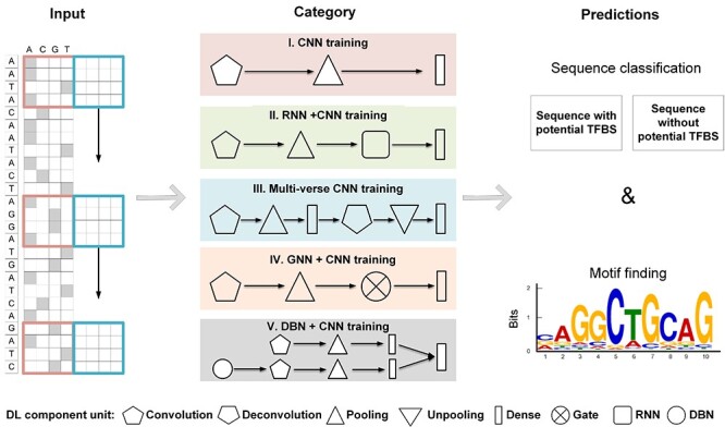
ChIP-seq data input and five categories of DL methods. Outcomes include both predicted sequence labels and identified motif patterns.

Category I: CNN-based methods maintain the simplest architecture that includes a convolutional layer, a pooling layer and a dense layer. One typical CNN-based tool is DeepBind [19], in which multiple convolutional kernels in the first CNN layer were set as motif detectors to scan the input sequences. DeepBind can be applied to both ChIP-seq and CLIP-seq data and outperformed most of the existing tools by the date it is published. Our DESSO [14] was then developed for motif prediction by CNN and motif occurrence optimization by a binomial distribution model. Key features of DESSO include: (i) it can predict not only sequence motifs but also DNA shape motifs, which improves in the identification and structural analysis of TFBSs; and (ii) it expands motif discovery by allowing the identification of known and new TF–TF–DNA tethering interactions in human. DeepHistone [28] integrated sequence information and chromatin accessibility data to accurately predict modification sites specific to different histone markers. It has been proved to effectively predict histone modification sites and recover TF binding motifs simultaneously. Zeng et al. [30] showcased that the useful addition of convolutional kernels is crucial for motif prediction in a CNN. DeepSEA [20] was developed for estimating noncoding-variant effects on chromatin with three tasks: integrating sequence information from a broad sequence context, learning sequence patterns at multiple spatial scales with a hierarchical architecture, and multi-task joint learning of diverse chromatin factors sharing predictive features. Other tools in this category include Basset [27], iDeepV [37], iDeepE [7], DeFine [29], DANN_TF [31] and Deep-RBPPred [38].

Category II: This kind of tool deploys an integrative CNN and RNN in motif prediction. For example, DeeperBind [33] was built based on DeepBind, including a convolutional layer, a pooling layer, two long-short-term-memory layers and a dense layer. It can be trained with varying-length sequences to model the sequence dependencies. DanQ [35] was developed for predicting the function of non-coding genomic regions. The first convolutional layer was used to find motifs with the same strategy as DeepBind, and the RNN prompts DanQ to consider the orientations and spatial distance between motifs. WSCNNLSTM [36] was a weak-supervised framework that uses k-mer encoding to transform DNA sequences from the reference in testing data. It contains three steps: segmentation process and k-mer encoding for sequence preprocessing, a hybrid deep neural network of CNN and RNN for sequence classification, and a noise-fusion step. Other tools deploying a combinatory architecture of RNN and CNN include DeepCpG [34], iDeepS [39] and FactorNet [32].

The rest of the three categories only have been deployed on individual tools. Category III: DeepSNR [21] uses a multi-verse training framework to predict TFBSs from DNA sequences, containing a basic convolutional layer, a deconvolutional layer, a pooling layer, an unpooling layer and a fully connected layer. It was trained using TF-specific data from ChIP-exonuclease experiments and can be used to identify TFBSs. Category IV: TFImpute [22] deploys a gate layer after the pooling layer of CNN and embeds cell lines and TFs into continuous vectors that serve as part of the model input. The unique imputation ability offered by the gate layer further extends the predictive power to TF-cell line combinations without the use of corresponding ChIP-seq data. Category V: iDeep [40] is a combination of DBN and CNN models and operation in a parallel manner and is the only one deployed such an architecture in the public domain.

Computational evaluation design for the 20 DL tools

We benchmarked the motif prediction performance of 20 DL tools in analyzing DNA and RNA sequences, respectively (Figure 2). To systematically compare the 20 tools, we used four metrics to assess their performances from multiple aspects: (i) an area of eight metrics radar (AEMR) score defines the accuracy of sequence classification. AEMR is based on F1_score, recall, precision, precision-recall curve (PRC), area under the curve (AUC), Matthews correlation coefficient (MCC), specificity and accuracy (ACC) (see detail in section ‘Evaluation criteria for sequence classification’); (ii) a motif prediction score to assess the significance and accuracy of identified motifs; (iii) method scalability of running time performed on different data scales and (iv) usability of the tool in terms of the tutorial, updates, code quality, etc. Considering the importance of each metric, we allocated weights of 0.3, 0.3, 0.2 and 0.2 to each of the four metrics, respectively. The weighted four metrics were summed up as an overall score used to assess the overall performance of these tools, with gkmSVM and MEME-ChIP as two traditional tools for the result comparison [41].

Figure 2.

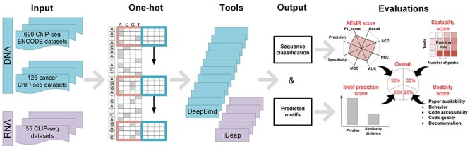
Schematic overview of the evaluation pipeline. AEMR score assesses the sequence classification ability based on F1_score, recall, precision, PRC, AUC, MCC, specificity and ACC between predicted classification labels and ChIP-seq peak labels. The motif prediction score (with a P-value and a similarity) assesses how well the predicted motifs can be, based on the documented TFBSs.

Dataset description

The 690 ChIP-seq datasets were obtained from ENCODE, covering 161 TFs and covered 91 human cell types. We selected the sequences with a length of 1001 bps as the input. Meanwhile, we collected 55 CLIP-seq datasets from references [37] and used a fixed length of 101 bps as input, as used in iDeep [40]. The Cistrome Data Browser was used to query the human cancer ChIP-seq datasets and 126 cancer ChIP-seq of nine cancer types were selected as (i) the corresponding cell line should be a cancer cell, and (ii) the quality control standards of the peaks must be high. All the above datasets, except the CLIP-seq data, only contained positive samples (peak sequences). Peaks in each dataset are ranked in the decreasing order of their signal scores. The top 500 odd peaks in each dataset are selected to test DL models; 80% of the rest of the peaks are selected to train the model, and the remaining ones are used for validation. The negative samples are selected based on: (i) having matched GC-content as the same as positive samples and (ii) not overlapping with any peaks in the positive samples. To avoid sample bias, the number of negative samples is equal to the number of positive samples. All positive samples were labeled as ‘1’, and negative samples as ‘0’.

As DL methods require binary vector as input, each input sequence was converted to an encoded matrix , i.e., , , , where is the length of input sequence [42]. We pruned the original peak with a fixed length (101 or 1001 bps) by formula (1). The position of the processed peak in the chromosome can be identified by

(1)

where is the start position of the original peak is the end position of the original peak position. After pruning, redundant peaks can be generated but were removed in the experiment, and the bedtools v2.21.0 were employed to acquire the pruned sequences [43]. The pruned sequences were encoded in the same way for CLIP-seq data as ChIP-seq data.

DL model training

The first layer kernel of a model was recognized as motif detectors, recognizing activated sequence fragments by scanning across the input matrix . The convolutional vector is defined as

(2)

where represents activation function; is ith convolutional kernel and is the threshold value. The number of convolutional kernels for each DL model differs by application. Each value of the vector represents the convolutional result, and the maximum value of is considered to be the activated score of sequence fragment. A classification layer will then classify each sequence fragment as positive or negative. A DL model is trained by applying labeled negative and positive samples in the training data. Motifs are represented by position weight matrix (PWM), which is a set of aligned activated sequence fragments. A PWM can be generated with rows as the four nucleic acid types (i.e. A, T/U, C and G), columns as sequence positions and an element as nucleotide occurrences in the corresponding position [44].

Evaluation criteria for sequence classification

To evaluate the performance of DL methods in sequence classification, we defined the AEMR score. The AEMR included the precision, recall, F1_score, specificity, ACC, MCC, AUROC and AUPRC, which assessed the model’s ability in identifying positive and negative samples and classifying DNA/RNA sequences. The above eight metrics are defined as follows.

Precision is the ratio of the true predicted positive samples to all the predicted positive samples. The higher the score, the greater the number of correct positive samples predicted by the model.

(3)

The recall represents the proportion of positive samples correctly predicted to the total positive samples. The higher the score, the greater the proportion of the positive samples identified by the model to the real positive samples.

(4)

F1_score is the harmonic mean of precision and recall.

(5)

Specificity is the proportion of identified negative samples to all negative samples, which indicates the model’s ability to identify negative samples.

(6)

ACC is the proportion of correct prediction to the total sample. The higher the score, the model predicts correctly.

(7)

MCC is essentially the correlation coefficient between the observed and the predicted; it is a value between −1 and +1. The coefficient +1 means perfect prediction, 0 means no better than a random prediction and −1 means discrepancy between prediction and observation.

(8)

AUROC is the area under the receiver operating characteristic curve, which is a value between 0 and 1. The closer AUROC is to 1, the better the classification is. The higher the score, the better the classification ability of the model.

AUPRC is the area under the PRC, which also is a value between 0 and 1. The difference between AUROC and AUPRC is that when the positive and negative samples are unbalanced, AUPRC is more sensitive to experimental results.

We then aggregated the eight scores into the AEMR score. Specifically, a radar chart can be generated consisting of eight equiangular spokes, with each spoke representing one of the scores defined above. The length of a spoke is proportional to the magnitude of the score for the data point relative to the maximum magnitude of the score across all data points. The AEMR score is the total area of the octagonal radar and is scaled to a score ranging from 0 to 1. The higher the AEMR score is, the better performance the tool has for sequence classification.

Evaluation criteria for motif prediction

To ensure a low false-positive rate, we used both TOMTOM and TFBSTools to evaluate the motif prediction results of the 20 DL tools. For each query motif, TOMTOM (v5.1.0) measures the similarity significance via motif comparisons between a query motif and the motif in the HOCOMOCO (V11) database [45, 46]. However, previous studies have reported TOMTOM might generate lots of false positives when matching the position probability matrix against a motif database [11]. TFBSTools compares the similarity between the PWM of the predicted motif and the PWM of TFBS in database by computing the Euclidean distance [47]. To this order, we use TFBSTools to calculate the similarity between the PWMs of the predicted motif and the documented TFBS based on the aggregation of Euclidean distance per base pair. TFBSs with the lowest average Euclidean distances to the predicted motif are considered as the matched TFBSs. For each DL method, we calculate the motif prediction score as

(9)

where is the significance of similarity significance in TOMTOM, and is the Euclidean distance calculated in TFBSTools. Both and are scaled to the range of 0–1 by dividing the maximum values, respectively. Note that, we only keep motifs that can be matched with existing motif patterns in the database using TOMTOM and TFBSTools.

Evaluation of tool efficiency

To assess the scalability of each method, we started from four kinds of real datasets, each of which contained 10 sub-datasets with a fixed number of peaks as 10, 20, 30 and 40 k, respectively. We run each tool on the four kinds of datasets for 300 min as a maximum. To determine the training time of each model in a fair way, we started the timer after loading data and the package and stopped the timer after finishing the training process. Furthermore, we normalized the training time of all tools for the same dataset by setting the slowest (i.e. 300 min) as 0, the quickest as 1 and re-scaling the others accordingly. The scalability score was defined as the average of the normalized training time in all four datasets.

Evaluation of tool usability

The usability of each model was quantified based on several existing model quality and programming guidelines [48]. It covers availability, behavior, code assurance, code quality and documentation categories. Specifically, availability checks whether the packages and dependencies can be easily installed and whether the method is readily available and used. Code quality is assessed both from a user perspective and a developer perspective. The code assurance category is frequently checked for code testing, continuous integration and an active maintaining team. Documentation checks whether the tool can provide helpful guidelines and clear tutorials. Finally, behavior evaluates the ease by which the method can be run by looking for unexpected output files, messages and prior information. We also assigned a weight to the individual aspect being investigated [48], and each of the five categories was weighted equally for calculating the final score.

RESULTS

Evaluation results on ChIP-seq and CLIP-seq data

Based on the above four metrics, an overall score was calculated to assess the performance of the 20 tools (Supplementary Figures S1 and S2, and Supplementary Tables S1–S4 available online at http://bib.oxfordjournals.org/). As shown in Figure 3, the performance of these tools differed substantially in the AEMR scores, motif prediction scores and tool usability, while the method scalability scores moderately varied. Among all the DL tools, our DESSO achieves the highest overall score for DNA sequence-based analysis, and iDeep is the best-performing tool for RNA sequence-based analysis. Interestingly, our results showcased that CNN-based tools tend to have better performance than tools in other categories for DNA sequence-based analysis, while on the contrary, for RNA sequence-based analysis. We reasoned that such results might be due to insufficient data training and more noises in CLIP-seq data compared with ChIP-seq data.

Figure 3.

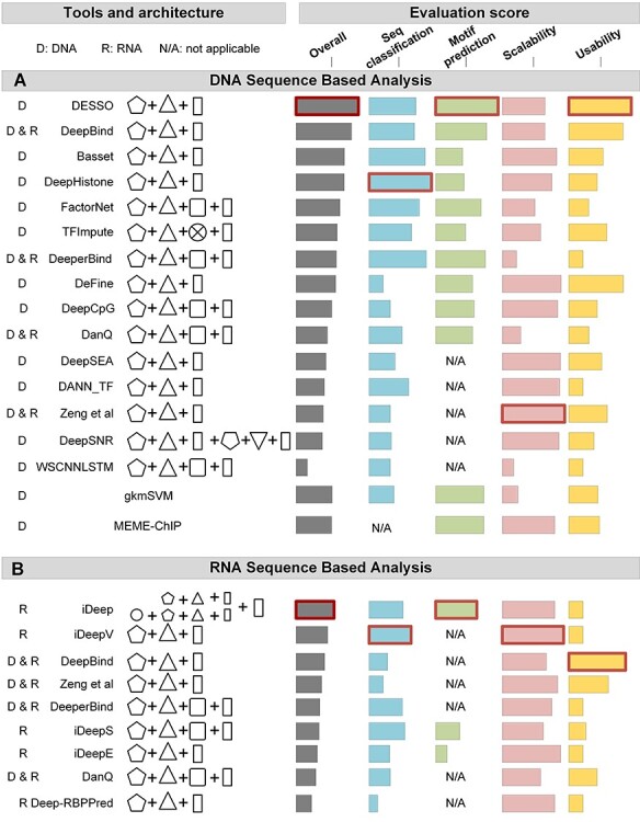
Illustration of evaluation results for the 20 DL tools. (A) For DNA sequence-based analysis, tools were separated by DL methods. In each comparative group, tools were ranked by their overall score (grey) from high to low. Four evaluation scores were shown: AEMR (blue), motif prediction score (green), algorithm scalability (pink) and tool usability (yellow). The highest score for each evaluation score is highlighted in a red box. The result of the conventional method gkmSVM and MEME-ChIP was also shown at the bottom for comparison. (B) For RNA sequence-based analysis, the same columns and labels were used as described in A.

As shown in Figure 3A, for DNA sequence training, DeepHistone showed the best performance in terms of the AEMR score. The stacked three convolutional layers in DeepHistone as a convolutional block may contribute to extract sequence information more effectively than a single layer convolution. We also selected gkmSVM [49] and MEME-ChIP, two popular traditional methods for motif prediction, as comparison tools. For the 15 DL methods conducted on the DNA sequence analysis, 10 of them showed better sequence classification performance than gkmSVM, while only DESSO achieved higher motif prediction results than gkmSVM (i.e. the best tool among all 15 DL methods). We reasoned that, other than convolutional kernels, DESSO also integrates the binomial distribution to optimize the TFBS identification based on identified motif patterns. Five out of 15 DL tools available for DNA sequence-based analysis lack the ability to predict motifs from ChIP-seq data (annotated as N/A in Figure 3A), leading to lower overall scores than the others. Running times were recorded by applying each tool for different peak numbers from 10 to 40 k, with a range of 10 k. All CNN-based tools showed higher scalability scores than hybrid network tools, except for DeepCpG, which runs faster and steadily for large dataset analysis. Tools that only perform DNA sequence classification have an obvious advantage in achieving better scalability scores. DESSO is considered to be the easiest accessible tool with a user-friendly webserver and detailed documentations, while most tools with only packages available usually need more effort in installation and environment settings.

Showcased in Figure 3B, for RNA sequence training, iDeepV and iDeep represent the best tool for RNA sequence classification and RNA motif identification, respectively. iDeep uses a multimodal framework that employing parallel DBN and CNN models and integrating the different sequence features captured on both sides, which augments the representation of the sequence. On the other hand, iDeepV uses the embedding layer to encode the input sequences, which aids the CNN layer to effectively learn the features of the sequence. DeepBind is under good maintenance with detailed tutorial documentation, especially for RNA sequence-based analysis.

Assess DL methods on nine cancer types

TFs have been proven to take part in carcinogenesis, cancer development [50] and defining aberrant gene expression in cancer cells [2]. We are interested in how the 15 DL tools for DNA sequences can derive new insights from cancer-related ChIP-seq data. An overview result showcased that the performance of sequence classification was highly variable across tools, and TFImpute had the highest performance among all the tools (Figure 4A, Supplementary Figure S3 available online at http://bib.oxfordjournals.org/). We reasoned that the reserve and forget mechanism of gates can contribute to keeping true signals and filter noises along with iteration processes, which is especially suitable for cancer datasets containing more sequence mutations than normal tissue data. DeepHistone and DeepBind performed better than other tools on liver cancer and lung cancer data, respectively. It is noteworthy that, the rank of the 11 tools that can deliver motif predictions on cancer data, in terms of classification performance, is consistent with the performance rank on the benchmark data, indicating the robustness of our benchmark design in the above sections. On the other hand, consistent classification performances across cancer types of each tool show that these tools performed steadily on different datasets.

Figure 4.

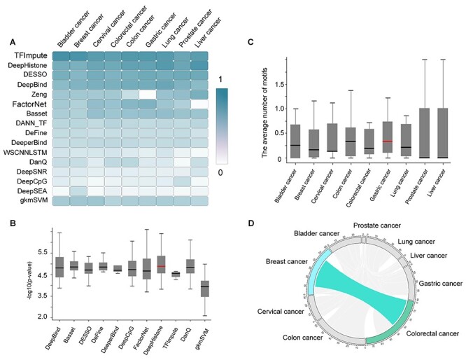
Analysis of motif analysis on nine cancer types. (A) AEMR scores of the 15 DL methods across the nine cancer types. (B) Box plot of motif enrichment P-value (with details in the Method section) of 11 methods with respect to breast cancer. (C) For each cancer type, we calculate the average number of identified motifs for each tool. Note that, we only keep motifs that can be matched with existing motif patterns in the database using TOMTOM and TFBSTools. The horizontal red line indicates the highest median value on the y-axis. (D) The shared motifs between the nine different cancer types. Motifs shared between breast cancer and colorectal cancer were highlighted as cyan, and all other shared links were light grey.

For all the identified motifs from the cancer datasets, we performed motif clustering using similarity scores from TOMTOM, and the most significant motif in terms of its P-value in each cluster was defined as the representative motif. Eventually, 132 representative motifs were identified from all the 126 cancer datasets for the following analyses. For an individual cancer type, significant diversities and variances of motif prediction performance were observed among different tools, in which TFImpute had the lowest variance and most robustness, and DeepHistone showed the highest mean performance (Figure 4B). The average number of predicted motifs across nine cancer types varied, and apparently, there was a lower number of predicted motifs in prostate cancer and liver cancer than those in the other seven cancer types (Figure 4C and Supplementary Table S5 available online at http://bib.oxfordjournals.org/). This may be due to the less known motifs identified for these two cancer types than other types.

To understand the overlap and uniqueness status of the identified 132 motifs, we used colorectal cancer as an example to discover its shared motifs with other cancer types. Of all 77 motifs identified in colorectal cancer, 38 of them were also identified in breast cancer data. For example, STAT3 [51, 52], FOXO3 [53, 54] and FOXP1 [55, 56] have been proven to play similar roles in breast and colorectal cancer. Of all the 132 identified motifs, only 62 motifs are unique to their corresponding cancer type, and the other 70 motifs were identified in two or more cancer types (Figure 4D). Those uniquely identified motifs might be the key to determine gene signatures that play essential roles in the occurrence and development of the specific cancer type. For example, ETV1 uniquely identified in breast cancer was found to have a higher expression level compared with normal tissues, while the overexpression of COP1 led to a significant expression level of ETV1 and suppressed cell migration and invasion [57]. Motif related to KLF4 identified in colorectal cancer is a zinc finger TF, which has been confirmed to be a tumor suppressor gene [58].

DISCUSSIONS

In this study, we reviewed and presented a large-scale performance evaluation of 20 DL methods for de novo motif prediction. Our benchmarking study provided a practical model and a set of optimal DL strategies for different datasets (ChIP-seq and CLIP-seq) in terms of the accuracy of motif finding, the performance of DNA/RNA sequence classification, method scalability and tool usability. The existing methods were assessed to be highly complementary to each other, and the most suitable method will be context-specific, which primarily depends on the data size and type as well as the method outputs. Specifically, we observed that CNN-based tools were better performed than other tools for DNA sequence and motif analysis while performs worse than others for RNA sequence and motif analysis. DESSO and iDeep are the best tools for DNA and RNA sequence, respectively, in terms of the above four metrics. The result proved that the convolutional operation could improve the performance of TF-DNA binding specificity prediction through optimizing the position-weight-matrix-like motif detectors. We further applied 11 tools on 126 cancer data and found TFImpute performs as the most robust tool for sequence classification and motif prediction across all nine cancer types. These tools showed less sequence classification bias among ChIP-seq data of different cancer types while exhibiting differences in the number and type of predicted enriched motifs. Only a few motifs are uniquely identified in each cancer type which might be caused by the heterogeneous nature of cancer cells. The shared motifs may shed light on the shared regulatory mechanism and pathways in different cancer types, leading a potential way to the study of drug repositioning.

Some practical challenges were also presented through the above evaluation studies. First, the comparison results suggested that the existing models presented unstable performances for the 126 ChIP-seq datasets obtained from nine cancer types. Hence, more efforts are needed to select a suitable tool or an appropriate combination of tools for motif prediction and sequence classification in different cancer types. Secondly, the convolutional kernel was used as the detector to scan the input sequence; however, the number of kernels and the width of a specific kernel were quite differently set up among the reviewed tools and affected the prediction performance. For example, the number of kernels exceeded 100 in some DL methods, which consumes too much computing resources and produces redundant results in ChIP-seq data. Hence, such necessary parameters should be well adjusted based on the tutorial of the selected tool or automatically trained by the meta-learning techniques [59]. Thirdly, most CNN methods outperform other methods and usually have lower computational complexity. There is still room for the integration of diverse neural network structures and strategies in a unified framework or an ensemble learning manner [60, 61].

In summary, new insights and computational infrastructures can significantly facilitate researchers in selecting the appropriate tools for their analyses related to motif finding and gene regulation. Overall, the ‘good-yet-not-the-best’ methods can still provide a valuable contribution to motif finding when one takes advantage of novel algorithms, proposes a more scalable solution or provides a unique insight in specific use cases. On the other hand, combining different tools in one analysis is always beneficial based on the observed complementarity of the evaluated DL methods in our study.

Data availability

The 690 ChIP-seq data can be downloaded from http://bmbl.sdstate.edu/DESSO/. The assessable links and accession number of the 55 CLIP-seq and 126 cancer ChIP-seq datasets used in this study can be retrieved in Supplementary Tables S6 and S7 available online at http://bib.oxfordjournals.org/. All source codes of the 20 DL methods can be found on GitHub, with links listed on https://github.com/OSU-BMBL/deepmotif-benchmark.

Key Points

• Identifying cis-regulatory motifs from genomic sequencing data is crucial in identifying transcription factor (TF) binding sites and inferring gene regulatory mechanisms for any organism. Without a clear and systematic assessment, users will struggle in choosing the most appropriate DL tool for their specific studies.

• We reviewed 20 existing DL methods for cis-regulatory motif prediction and delivered in-depth insights via comprehensive benchmark evaluations of their performances.

• The experimental results indicated the high complementarity of the existing DL methods, and the most suitable model users select should primarily depend on the data size and type as well as the method’s outputs.

Shuangquan Zhang is a Ph.D. candidate at College of Computer Science and Technology, Jilin University. He is interested in developing deep learning methods for motif finding.

Anjun Ma, PhD, is a Postdoc at the Ohio State University. His research focuses on developing computational tools for single-cell data analysis, gene regulation network construction in immuno-oncology, involving deep learning algorithms.

Jing Zhao, PhD, is a Research Scientist in the Department of Biomedical Informatics at the Ohio State University. Her research interests are machine learning-based biomedical data analysis.

Dong Xu, PhD, is a Professor in the Electrical Engineering and Computer Science Department at the University of Missouri. His research is in computational biology and bioinformatics, including machine-learning application in bioinformatics, protein structure prediction, post-translational modification prediction and high-throughput biological data analyses.

Qin Ma, PhD, is an Associate Professor at the Department of Biomedical Informatics, the Ohio State University. His is interested in (i) understanding of how functional machinery encoded in a genome, (ii) elucidation of the underlying regulatory mechanisms of complex diseases using single-cell data and (iii) development of enabling computational techniques

Yan Wang, PhD, is a Professor at the Key Laboratory of Symbol Computation and Knowledge Engineering of Ministry of Education, College of Computer Science and Technology, Jilin University. His research focuses on developing deep learning methods and analyzing omics data.

Authors’ contributions

Q.M. designed the study. S.Z. and J.Z. performed the experiments. Y.W., S.Z., J.Z., D.X. and A.M prepared the manuscript. Y.W. and Q.M. supervised the project.

Funding

National Natural Science Foundation of China (62072212, 61772227); the Development Project of Jilin Province of China (20200401083GX, 2020C003); Guangdong Key Project for Applied Fundamental Research (2018KZDXM076); and Jilin Provincial Key Laboratory of Big Data Intelligent Computing (20180622002JC).

References

- 1. Lin Quy Xiao X, Thieffry D, Jha S, et al. TFregulomeR reveals transcription factors’ context-specific features and functions. Nucleic Acids Res 2019;48:e10–0. [DOI] [PMC free article] [PubMed] [Google Scholar]
- 2. Bhagwat AS, Vakoc CR. Targeting transcription factors in cancer. Trends Cancer 2015;1:53–65. [DOI] [PMC free article] [PubMed] [Google Scholar]
- 3. D'haeseleer P. What are DNA sequence motifs? Nat Biotechnol 2006;24:423–5. [DOI] [PubMed] [Google Scholar]
- 4. Chen H, Li H, Liu F, et al. An integrative analysis of TFBS-clustered regions reveals new transcriptional regulation models on the accessible chromatin landscape. Sci Rep 2015;5:8465. [DOI] [PMC free article] [PubMed] [Google Scholar]
- 5. Zambelli F, Pesole G, Pavesi G. Motif discovery and transcription factor binding sites before and after the next-generation sequencing era. Brief Bioinform 2013;14:225–37. [DOI] [PMC free article] [PubMed] [Google Scholar]
- 6. Kharchenko PV, Tolstorukov MY, Park PJ. Design and analysis of ChIP-seq experiments for DNA-binding proteins. Nat Biotechnol 2008;26:1351–9. [DOI] [PMC free article] [PubMed] [Google Scholar]
- 7. Pan X, Shen H-B. Predicting RNA–protein binding sites and motifs through combining local and global deep convolutional neural networks. Bioinformatics 2018;34:3427–36. [DOI] [PubMed] [Google Scholar]
- 8. Guo Y, Tian K, Zeng H, et al. A novel k-mer set memory (KSM) motif representation improves regulatory variant prediction. Genome Res 2018;28:891–900. [DOI] [PMC free article] [PubMed] [Google Scholar]
- 9. Yang J, Chen X, McDermaid A, et al. DMINDA 2.0: integrated and systematic views of regulatory DNA motif identification and analyses. Bioinformatics 2017;33:2586–8. [DOI] [PubMed] [Google Scholar]
- 10. Machanick P, Bailey TL. MEME-ChIP: motif analysis of large DNA datasets. Bioinformatics 2011;27:1696–7. [DOI] [PMC free article] [PubMed] [Google Scholar]
- 11. Koo PK, Eddy SR. Representation learning of genomic sequence motifs with convolutional neural networks. PLoS Comput Biol 2019;15:e1007560. [DOI] [PMC free article] [PubMed] [Google Scholar]
- 12. Liu B, Yang J, Li Y, et al. An algorithmic perspective of de novo cis-regulatory motif finding based on ChIP-seq data. Brief Bioinform 2018;19:1069–81. [DOI] [PubMed] [Google Scholar]
- 13. Ma A, Wang C, Chang Y, et al. IRIS3: integrated cell-type-specific regulon inference server from single-cell RNA-Seq. Nucleic Acids Res 2020;48:W275–86. [DOI] [PMC free article] [PubMed] [Google Scholar]
- 14. Yang J, Ma A, Hoppe AD, et al. Prediction of regulatory motifs from human ChIP-sequencing data using a deep learning framework. Nucleic Acids Res 2019;47:7809–24. [DOI] [PMC free article] [PubMed] [Google Scholar]
- 15. Fornes O, Castro-Mondragon JA, Khan A, et al. JASPAR 2020: update of the open-access database of transcription factor binding profiles. Nucleic Acids Res 2020;48:D87–d92. [DOI] [PMC free article] [PubMed] [Google Scholar]
- 16. Wingender E, Dietze P, Karas H, et al. TRANSFAC: a database on transcription factors and their DNA binding sites. Nucleic Acids Res 1996;24:238–41. [DOI] [PMC free article] [PubMed] [Google Scholar]
- 17. Matys V, Fricke E, Geffers R, et al. TRANSFAC: transcriptional regulation, from patterns to profiles. Nucleic Acids Res 2003;31:374–8. [DOI] [PMC free article] [PubMed] [Google Scholar]
- 18. Kulakovskiy IV, Vorontsov IE, Yevshin IS, et al. HOCOMOCO: towards a complete collection of transcription factor binding models for human and mouse via large-scale ChIP-seq analysis. Nucleic Acids Res 2018;46:D252–9. [DOI] [PMC free article] [PubMed] [Google Scholar]
- 19. Alipanahi B, Delong A, Weirauch MT, et al. Predicting the sequence specificities of DNA- and RNA-binding proteins by deep learning. Nat Biotechnol 2015;33:831–8. [DOI] [PubMed] [Google Scholar]
- 20. Zhou J, Troyanskaya OG. Predicting effects of noncoding variants with deep learning-based sequence model. Nat Methods 2015;12:931–4. [DOI] [PMC free article] [PubMed] [Google Scholar]
- 21. Salekin S, Zhang JM, Huang Y. Base-pair resolution detection of transcription factor binding site by deep deconvolutional network. Bioinformatics 2018;34:3446–53. [DOI] [PMC free article] [PubMed] [Google Scholar]
- 22. Qin Q, Feng J. Imputation for transcription factor binding predictions based on deep learning. PLoS Comput Biol 2017;13:e1005403. [DOI] [PMC free article] [PubMed] [Google Scholar]
- 23. Min S, Lee B, Yoon S. Deep learning in bioinformatics. Brief Bioinform 2017;18:851–69. [DOI] [PubMed] [Google Scholar]
- 24. Yang F, Du C, Huang L. Ensemble sentiment analysis method based on R-CNN and C-RNN with fusion gate. Int J Comput Commun Cont 2019;14:272–85. [Google Scholar]
- 25. Chen Y, Zhao X, Jia X. Spectral–spatial classification of hyperspectral data based on deep belief network. IEEE J Sel Top Appl Earth Obs Remote Sens 2015;8:2381–92. [Google Scholar]
- 26. Tran HTN, Ang KS, Chevrier M, et al. A benchmark of batch-effect correction methods for single-cell RNA sequencing data. Genome Biol 2020;21:1–32. [DOI] [PMC free article] [PubMed] [Google Scholar]
- 27. Kelley DR, Snoek J, Rinn JL. Basset: learning the regulatory code of the accessible genome with deep convolutional neural networks. Genome Res 2016;26:990–9. [DOI] [PMC free article] [PubMed] [Google Scholar]
- 28. Yin Q, Wu M, Liu Q, et al. DeepHistone: a deep learning approach to predicting histone modifications. BMC Genomics 2019;20:193. [DOI] [PMC free article] [PubMed] [Google Scholar]
- 29. Wang M, Tai C, Weinan E, et al. DeFine: deep convolutional neural networks accurately quantify intensities of transcription factor-DNA binding and facilitate evaluation of functional non-coding variants. Nucleic Acids Res 2018;46:e69–9. [DOI] [PMC free article] [PubMed] [Google Scholar]
- 30. Zeng H, Edwards MD, Liu G, et al. Convolutional neural network architectures for predicting DNA–protein binding. Bioinformatics 2016;32:i121–7. [DOI] [PMC free article] [PubMed] [Google Scholar]
- 31. Lan G, Zhou J, Xu R, et al. Cross-cell-type prediction of TF-binding site by integrating convolutional neural network and adversarial network. Int J Mol Sci 2019;20:3425. [DOI] [PMC free article] [PubMed] [Google Scholar]
- 32. Quang D, Xie X. FactorNet: a deep learning framework for predicting cell type specific transcription factor binding from nucleotide-resolution sequential data. Methods 2019;166:40–7. [DOI] [PMC free article] [PubMed] [Google Scholar]
- 33. Hassanzadeh HR, Wang MD. DeeperBind: enhancing prediction of sequence specificities of DNA binding proteins. In: 2016 IEEE International Conference on Bioinformatics and Biomedicine (BIBM). IEEE (Institute of Electrical and Electronics Engineers), 2016, p. 178–83. [DOI] [PMC free article] [PubMed]
- 34. Angermueller C, Lee HJ, Reik W, et al. DeepCpG: accurate prediction of single-cell DNA methylation states using deep learning. Genome Biol 2017;18:67. [DOI] [PMC free article] [PubMed] [Google Scholar]
- 35. Quang D, Xie X. DanQ: a hybrid convolutional and recurrent deep neural network for quantifying the function of DNA sequences. Nucleic Acids Res 2016;44:e107. [DOI] [PMC free article] [PubMed] [Google Scholar]
- 36. Zhang Q, Shen Z, Huang D-S. Modeling in-vivo protein-DNA binding by combining multiple-instance learning with a hybrid deep neural network. Sci Rep 2019;9:8484. [DOI] [PMC free article] [PubMed] [Google Scholar]
- 37. Pan X, Shen H-B. Learning distributed representations of RNA sequences and its application for predicting RNA-protein binding sites with a convolutional neural network. Neurocomputing 2018;305:51–8. [Google Scholar]
- 38. Zheng J, Zhang X, Zhao X, et al. Deep-RBPPred: predicting RNA binding proteins in the proteome scale based on deep learning. Sci Rep 2018;8:15264. [DOI] [PMC free article] [PubMed] [Google Scholar]
- 39. Pan X, Rijnbeek P, Yan J, et al. Prediction of RNA-protein sequence and structure binding preferences using deep convolutional and recurrent neural networks. BMC Genomics 2018;19:511. [DOI] [PMC free article] [PubMed] [Google Scholar]
- 40. Pan X, Shen H-B. RNA-protein binding motifs mining with a new hybrid deep learning based cross-domain knowledge integration approach. BMC Bioinformatics 2017;18:136. [DOI] [PMC free article] [PubMed] [Google Scholar]
- 41. Maulik U, Mukhopadhyay A, Bandyopadhyay S. Combining Pareto-optimal clusters using supervised learning for identifying co-expressed genes. BMC Bioinformatics 2009;10:27. [DOI] [PMC free article] [PubMed] [Google Scholar]
- 42. Jinyu Y, Anjun M, Hoppe AD, et al. Prediction of regulatory motifs from human ChIP-sequencing data using a deep learning framework. Nuclc Acids Res 2019;15:7809–7824. [DOI] [PMC free article] [PubMed] [Google Scholar]
- 43. Quinlan AR, Hall IM. BEDTools. Curr Protoc Bioinformatics 2016;47:11.12.11. [DOI] [PMC free article] [PubMed] [Google Scholar]
- 44. Crooks GE, Hon G, Chandonia J-M, et al. WebLogo: a sequence logo generator. Genome Res 2004;14:1188–90. [DOI] [PMC free article] [PubMed] [Google Scholar]
- 45. Ma W, Noble WS, Bailey TL. Motif-based analysis of large nucleotide data sets using MEME-ChIP. Nat Protoc 2014;9:1428–50. [DOI] [PMC free article] [PubMed] [Google Scholar]
- 46. Hartmann H, Guthöhrlein EW, Siebert M, et al. P-value-based regulatory motif discovery using positional weight matrices. Genome Res 2013;23:181–94. [DOI] [PMC free article] [PubMed] [Google Scholar]
- 47. Tan G, Lenhard B. TFBSTools: an R/bioconductor package for transcription factor binding site analysis. Bioinformatics 2016;32:1555–6. [DOI] [PMC free article] [PubMed] [Google Scholar]
- 48. Saelens W, Cannoodt R, Todorov H, et al. A comparison of single-cell trajectory inference methods. Nat Biotechnol 2019;37:547–54. [DOI] [PubMed] [Google Scholar]
- 49. Ghandi M, Mohammad-Noori M, Ghareghani N, et al. gkmSVM: an R package for gapped-kmer SVM. Bioinformatics 2016;32:2205–7. [DOI] [PMC free article] [PubMed] [Google Scholar]
- 50. Jiramongkol Y, Lam EW-F. FOXO transcription factor family in cancer and metastasis. Cancer Metastasis Rev 2020;39:1–29. [DOI] [PMC free article] [PubMed] [Google Scholar]
- 51. Banerjee K, Resat H. Constitutive activation of STAT3 in breast cancer cells: a review. Int J Cancer 2016;138:2570–8. [DOI] [PMC free article] [PubMed] [Google Scholar]
- 52. Rokavec M, Öner MG, Li H, et al. IL-6R/STAT3/miR-34a feedback loop promotes EMT-mediated colorectal cancer invasion and metastasis. J Clin Invest 2014;124:1853–67. [DOI] [PMC free article] [PubMed] [Google Scholar]
- 53. Ai B, Kong X, Wang X, et al. LINC01355 suppresses breast cancer growth through FOXO3-mediated transcriptional repression of CCND1. Cell Death Dis 2019;10:502. [DOI] [PMC free article] [PubMed] [Google Scholar]
- 54. Liu C, Zhao Y, Wang J, et al. FoxO3 reverses 5-fluorouracil resistance in human colorectal cancer cells by inhibiting the Nrf2/TR1 signaling pathway. Cancer Lett 2020;470:29–42. [DOI] [PubMed] [Google Scholar]
- 55. De Silva P, Garaud S, Solinas C, et al. FOXP1 negatively regulates tumor infiltrating lymphocyte migration in human breast cancer. EBioMedicine 2019;39:226–38. [DOI] [PMC free article] [PubMed] [Google Scholar]
- 56. Linde DS, Sofie P, Olivier G, et al. Expression of FOXP1 and colorectal cancer prognosis. Lab Med 2015;46:299. [DOI] [PubMed] [Google Scholar]
- 57. Ouyang M, Wang H, Ma J, et al. COP1, the negative regulator of ETV1, influences prognosis in triple-negative breast cancer. BMC Cancer 2015;15:132. [DOI] [PMC free article] [PubMed] [Google Scholar]
- 58. Ma Y, Lin W, Liu X, et al. KLF4 inhibits colorectal cancer cell proliferation dependent on NDRG2 signaling. Oncol Rep 2017;38:975. [DOI] [PubMed] [Google Scholar]
- 59. Hospedales T, Antoniou A, Micaelli P, et al. Meta-learning in neural networks: a survey arXiv preprint. IEEE Trans Pattern Anal Mach Intell 2020;PP(99):1–1. [DOI] [PubMed] [Google Scholar]
- 60. Hansen LK, Salamon P. Neural network ensembles. IEEE Trans Pattern Anal Mach Intell 1990;12:993–1001. [Google Scholar]
- 61. Sun X, Liu Y, An L. Ensemble dimensionality reduction and feature gene extraction for single-cell RNA-seq data. Nat Commun 2020;11:5853. [DOI] [PMC free article] [PubMed] [Google Scholar]
Associated Data
This section collects any data citations, data availability statements, or supplementary materials included in this article.
Supplementary Materials
Data Availability Statement