Artificial intelligence knacks-based stochastic paradigm to study the dynamics of plant virus propagation model with impact of seasonality and delays

Abstract

The presented study deals with the exploitation of the artificial intelligence knacks-based stochastic paradigm for the numerical treatment of the nonlinear delay differential system for dynamics of plant virus propagation with the impact of seasonality and delays (PVP-SD) model by implementing neural networks backpropagation with Bayesian regularization scheme (NNs-BBRS). The PVP-SD model is represented with five classes-based ODEs systems for the interaction between insects and plants. The nonlinear PVP-SD model governs with five populations: S(t) susceptible plants, I(t) infected plants, X(t) susceptible insect vectors, Y(t) infected insect vectors and P(t) predators. Adams numerical procedure is adopted to generate the reference solutions of the nonlinear PVP-SD model based on the variety of cases by varying the plants bite rate due to vectors, vector bite rate due to plants, plant’s recovery rate, predator contact rate with healthy insects, predator contact rate with infected insects and death rate caused by insecticides. The approximate solutions of the nonlinear PVP-SD model are determined by executing the designed NNs-BBRS through different target and inputs arbitrary selected samples for the training and testing data. Validation of the consistent precision and convergence of the designed NNs-BBRS is efficaciously substantiated through exhaustive simulations and analyses on mean square error-based merit function, index of regression and error histogram illustrations.

Introduction

Plants play a crucial role in maintaining our planet’s ecosystem. They are the source of food both for humans and for many other species on earth. Plants have been used since long for medical purposes. The fibers they produce are utilized for the clothing and paper, while the wood is an indispensable for building material. In order to maintain a healthy environment, plants need to be healthy as well. Unfortunately, plants also contact many diseases, some of which are caused by insects, such as beetles, while others are caused by viruses.

Many African countries that lack economic development depend on cassava that is susceptible to the cassava mosaic virus. There have been outbreaks of this plant virus in Southeast Asia [1]. The tomato plant in India is another example of a plant with virus infection. Tomato leaf curl disease is caused by these viruses. It results in a curled leaf and possibly sterility of the plants [2]. Viral diseases damage the plants and often kill them, resulting in billions of dollars in damages every year due to virus-caused diseases [3]. During the transmission process, insects usually bite plants infected by the virus, become infected and bite susceptible plants, thereby infecting them. Insects react differently according to the season. During the warm months, they are very active, and in the cool months, they almost go dormant. Transport is required by viruses in order to move from one plant to another. This is typically accomplished by insect vectors. Approximately, 70 percent of plant viruses are transmitted by insects [4]. It must become infected by feeding on an infected plant acquiring the virus from it, and then spread it to another healthy plant. Transmission of both TLCD and cassava mosaic virus occurs through the same vector Bemisia tabaci. There have been numerous mathematical models developed to provide a detailed exposition of how to describe, analyze and predict agricultural epidemics of plant pathogens as a mean of developing and testing crop protection tactics and control strategies [5–8]. There have been a number of epidemiological models developed to analyze the population ecology of viral diseases, based on those used in human or animal epidemiology [9–14]. Modeling of host, virus, and vector interactions and their use to evaluate control strategies are discussed [15]. Xiaowei Jiang investigated the bifurcation as well as chaos for delay differential system [16]. Haileyesus Tessema Alemneh formulated the epidemic model to investigate the dynamical behavior of maize streak virus and developed the control strategies [17]. A number of papers have discussed at least two species for delayed or non-delayed predator–prey models [18–24]. It has been shown that the majority of epidemiological models can be represented as a system of differential equations, with time lags frequently included [25, 26]. Theoretical studies of plant disease rarely use delay differential equations. Numerous studies dealing with infections have used constant delays, representing either the infectious phase following the removal of infected individuals or the latency phase after the infection has passed [27]. Wang et al. presented the dynamics of a predator–prey model including distributed delay with respect to time and mutual interference [28]. Zhang et al. considered the model of vector-borne disease having two delays and involving reinfection and discussed the system equilibrium [29]. Darti et al. presented the numerical approach for the SIR epidemic model with a saturated incidence rate by using the non-standard finite difference method [30]. Zhang et al. considered a tobacco smoking model with delay and studied the dynamics by taking the delay as a bifurcation factor based on the Hopf bifurcation and local stability [31]. Alcaide et al. discussed hybridized viral infections, ecological and evolutionary factors in plants diseases [32]. Benito Chen-Charpentier transformed the model of plant virus transmission with delay and stated the model based on biochemical effects which is most practical for small groups [33]. An analysis is presented for the mosaic disease of Cassava transmitted by the whitefly vector [34, 35]. Pratiwi et al. presented the mosaic disease mathematical model of Jatropha curcas and controlling strategies with nutritional interference and insecticide [8]. Zhong et al. considered the modeling of the communication system and analyzed the coordinated and non-coordinated impact of frequency control inside the virtual power plants [36]. Waezizadeh et al. investigated the plant virus propagation model and its dynamics with multiple delays [37]. Debasis Mukherjee presented the plant’s diseases model caused by insects biting the plants as well as the natural opponents and also investigated the model in terms of feasibility of equilibria, boundedness, uniform persistence, and local as well as global stability concerns [38]. Fei et al. studied the epidemic model of vector-borne disease based on the resistance, exposed period of disease and nonlinear incidence rate [39]. Based on a discrete plant virus disease model with drilling and replanting, Luo et al. showed that the basic reproduction number acts as a threshold parameter in determining the global dynamics of the model [40]. Using a mathematical model, a three-species food chain system incorporating delay of toxicant uptake by prey populations has been analyzed [41]. There has been extensive research on epidemics models for plant diseases (see [42–46]). Recent research conducted by Benito M. Chen-Charpentier and Mark Jackson examined indirect and direct optimal control methods to propagate plant viruses over a seasonal period and delays [47].

The existing literature contains many intriguing techniques, all of which have their own merits, advantages and disadvantages, but it is imperative to exploit the AI-based stochastic paradigm for solving epidemic models of plant virus transmission. Different stochastic numerical techniques have been used to solve linear and nonlinear mathematical systems [48–55]. A number of recent and advanced applications of stochastic numerical techniques based on AI include analysis of Williamson nanofluid [56], pantograph differential equations including delay [57], autoregressive nonlinear systems [58], nano-fluidic nonlinear systems [59], system of power plant [60], magneto-hydrodynamic [61], financial model [62], Thomas–Fermi nonlinear singular system [63], bistatic systems of radar [64], plasma [65], solar energy [66], HIV infectious model [67], nonlinear eye model [68], heartbeat model [69], COVID-19 nonlinear models [70, 71] and model of mosquito [72]. Moreover, these stochastic numerical methods are widely utilized for dealing with complex fractional-order systems [73–76]. These factors are instigation for authors to investigate, interpret, and study stochastic numerical techniques for solving nonlinear PVP-SD model. The present study utilizes a neural networks backpropagated with the Bayesian regularization to investigate the dynamical behavior of the nonlinear PVP-SD model. According to the authors literature review, the numerical solution to the nonlinear PVP-SD model by using artificial intelligence (AI) knacks via neural networks backpropagation with Bayesian regularization scheme (NNs-BBRS) looks promising alternative to be implemented. Following are the innovative aspects of the presented research work in terms of salient features:

• A novel design AI knacks-based stochastic numerical technique is presented using Bayesian regularization networks to efficaciously investigate the dynamics of the nonlinear plant virus propagation with the impact of seasonality and delays (PVP-SD) model.

• The PVP-SD model dynamics is portrayed mathematically by five classes-based ODEs systems for the interaction between insects and plants in terms of their populations for susceptible and infected items as well as for predators.

• Efficacy of Adams numerical procedure is adopted to generate the reference solutions of the nonlinear PVP-SD model for different scenarios by varying the plants bite rate due to vectors, vector bite rate due to plants, plant’s recovery rate, predator contact rate with healthy insects, predator contact rate with infected insects and death rate caused by insecticides.

• Validation of the consistent precision and convergence of the designed NNs-BBRS is practicality substantiated through exhaustive simulation studies and analyses on mean square error-based merit function, index of regression and error histogram illustrations.

The organization of the rest portion of the article is as follows. The second section of the article consists of the mathematical description of the nonlinear PVP-SD model. The third section consists of the proposed methodology of the nonlinear PVP-SD model. The fourth section comprises the dynamics-based analysis of the nonlinear PVP-SD model through a distinct scenario. The fifth section contains conclusion on the basis of comprehensive analysis.

Mathematical model of plant virus propagation

Plant virus propagation can be modeled using the mathematical models described in [76–79], which has the structure of an epidemiological model based on vectors. It consists of six populations: S(t) susceptible plants, I(t) infected plants, R(t) recovered plants, X(t) susceptible insect vectors, Y(t) infected insect vectors and P(t) predators. Each variable specifies the population value at time t. The susceptible plants do not possess the disease themselves, but they might contact it from an infected vector. Viruses can be transmitted indirectly to susceptible plants by infected plants. A plant infected with a disease may either die or recover from it due to a defensive mechanism. Due to the viral infection, these plants may also die more often than susceptible plants. We also presume that when a plant dies either naturally or due to infection, it is instantly exchanged with new susceptible plant by the farm worker. By this supposition, the population as a whole remains constant and denoted by $N$. Its advantage is that we may use $\text{N}=S+I+R$ in the system of equations to exclude the recovered population as well as its conservation equation. Susceptible insects are not infected with the virus but can become infected by biting an infected plant. Viruses can be transmitted to susceptible plants by biting insects that are infected. It is assumed that the virus cannot spread vertically between plants or vectors. Additionally, the virus is assumed not to harm the vector, so it does not need to protect the virus against itself and retains the virus throughout its’ life. Consequently, infected and susceptible vectors both die at the same rate, regardless of whether they are killed by insecticides or predators. The virus does not infect it while eating an infected vector, and also it does not spread the virus. There are two delays included in the model according to the time it takes the virus in order to spread within a plant or vector. There is also a seasonal variation in insect and plant contact rates, with warmer months having a higher rate than cooler months. Therefore, the contact rate is assumed to be yearly. The same applies to growth rates of a vector. In addition, predators compete for insects afterward. There is a constraint of the predator–prey Holling type-2 in the interactions between vectors and plants, as well as between predators and vectors.

The mathematical model is expressed by the following delay differential system [47]:

$$\begin{array}{cc}\frac{\text{d}S}{\text{d}t}=\upsilon \left(N-S\right)+cI-\frac{\alpha \left(t\right)Y\left(t-{\xi }_1\right)}{1+\gamma Y\left(t-{\xi }_1\right)}S\left(t-{\xi }_1\right)\hfill & S\left(0\right)=S_0\\ \frac{\text{d}I}{\text{d}t}=\frac{\alpha \left(t\right)Y\left(t-{\xi }_1\right)}{1+\gamma Y\left(t-{\xi }_1\right)}S\left(t\right)-\left(c+\upsilon +\beta \right)I\hfill & I\left(0\right)=I_0\\ \frac{\text{d}X}{\text{d}t}=\mathrm{\Lambda }-\frac{{\alpha }_1\left(t\right)I\left(t-{\xi }_2\right)}{1+{\gamma }_{1}Y\left(t-{\xi }_2\right)}X\left(t-{\xi }_2\right)-\frac{d_{1}X}{1+{\gamma }_{3}X}P\left(t\right)-kX-c_{\mathit{in}}X\hfill & X\left(0\right)=X_0\\ \frac{\text{d}Y}{\text{d}t}=\frac{{\alpha }_1\left(t\right)I\left(t-{\xi }_2\right)}{1+{\gamma }_{1}Y\left(t-{\xi }_2\right)}X\left(t-{\xi }_2\right)-\frac{d_{2}Y}{1+{\gamma }_{3}Y}P\left(t\right)-kY-c_{\mathit{in}}Y\hfill & Y\left(0\right)=Y_0\\ \frac{\text{d}P}{\text{d}t}={\mathrm{\Lambda }}_p+\frac{{\gamma }_4{d}_{1}X}{1+{\gamma }_{3}X}P\left(t\right)+\frac{{\gamma }_4{d}_{2}Y}{1+{\gamma }_{3}Y}P\left(t\right)-\eta P\left(t\right)-\delta P^2\left(t\right)\hfill & P\left(0\right)=P_0\end{array}$$ 1

where

$$\begin{array}{cc}\hfill \alpha \left(t\right)& =\alpha \left(1+lcos\left(\frac{2\pi t}{365}\right)\right)\hfill \\ \hfill {\alpha }_1\left(t\right)& ={\alpha }_1\left(1+lcos\left(\frac{2\pi t}{365}\right)\right)\hfill \\ \hfill \end{array}$$

In the absence of seasonality, we use $l=0$, and $l=0.5$ when seasonality including. In Fig. 1, plants, insects and predators are shown interacting with each other. Inflows of the given population are indicated by solid arrows toward a state. The outflow of a population is shown by a solid arrow away from it. The transmission of the virus is shown as a dotted line from one population to another. The settings of parameters for nonlinear PVP-SD model is shown in Table 1 used for every case of this study as per [47]. After using numerical values for one of the case, the obtained mathematical form of system (1) is given as [47]:

$$\begin{array}{cc}& S^{\prime }\left(t\right)=100-0.000942S\left(t\right)I\left(t\right)+0.03R\left(t-{\eta }_3\right)-0.011S\left(t\right),\hfill \\ \hfill & E^{\prime }\left(t\right)=0.000942S\left(t\right)I\left(t\right)-0.04E\left(t-{\eta }_1\right)-0.01E\left(t\right),\hfill \\ \hfill & I^{\prime }\left(t\right)=0.04E\left(t-{\eta }_1\right)-0.01I\left(t\right)-0.025I\left(t-{\eta }_2\right),\hfill \\ \hfill & R^{\prime }\left(t\right)=0.025\left(t-{\eta }_2\right)+0.001S\left(t\right)-0.01R\left(t\right)-0.03R\left(t-{\eta }_3\right),\hfill \\ \hfill \end{array}$$ 2

along with initial conditions

$$S(0)=750,E\left(0\right)=2100,I(0)=2900,R(0)=4400$$ 3

Fig. 1.

Interaction between the plants, insects and predators of the nonlinear PVP-SD model

Table 1.

Parameters with description and values [47]

Parameters	Definition	Value
$N$	Population of plant hosts	63
$\alpha$	Plants bite rate due to vectors	0.01
${\alpha }_1$	Vector bite rate due to plants	0.01
$\gamma$	Plant saturation constant due to vectors	0.2
${\gamma }_1$	Saturation constant of vector due to plants	0.1
$\upsilon$	Plant’s death rate naturally	0.01
$k$	Vector’s natural death rate	0.2974
$\beta$	Plant’s recovery rate	0.01
$\mathrm{\Lambda }$	Vectors replenishing rate	10
$c$	Infected plants death rate due to the disease	0.2
$d_1$	Predator rate of contact with healthy insects	0.05
$d_2$	Rate of contact between predators and the infected insects	0.05
$\eta$	Death rate of predators naturally	0.05
$\delta$	Constant competition between the predators	0.01
${\gamma }_3$	Predators’ saturation caused by insects	0.01
${\gamma }_4$	Predator conversion rate due to insects	0.01
$c_{\text{in}}$	Death rate caused by insecticides	0–0.9
${\mathrm{\Lambda }}_{\text{p}}$	Addition rate of predators	0–10

Further, similar mathematical models for other cases can be formulated for the nonlinear PVP-SD model.

Proposed methodology

The following section provides a mathematical model together with execution matrices for the proposed technique. Mathematical modeling involves three phases: An initial dataset used as a reference solution are created by the knack of Adams numerical solver in phase one, formulation of two-layer framework of NNs-BBRS in phase two, NNs is trained through Bayesian regularization to calculate the approximate solution in phase three.

Adams method

The following section presents the Adams predictor corrector technique [80, 81] for the system (1). In order to enhance the accuracy level of the results, we have utilized the Adams technique. The accuracy was initially determined by using predictor solutions, and then numerical corrections are carried out using yardsticks obtained by the predictor solutions. The predictor corrector technique based on system (1) can be expressed in the following manner:

$$\begin{array}{cc}& \frac{\text{d}S}{\text{d}t}=f\left(t,S,Y,I\right),S\left(t_0\right)=S_0\hfill \\ \hfill & \frac{\text{d}I}{\text{d}t}=g\left(t,I,S,Y\right),I\left(t_0\right)=I_0\hfill \\ \hfill & \frac{\text{d}X}{\text{d}t}=g\left(t,X,P,I\right),X\left(t_0\right)=X_0\hfill \\ \hfill & \frac{\text{d}Y}{\text{d}t}=g\left(t,Y,P,X,I\right),Y\left(t_0\right)=Y_0\hfill \\ \hfill & \frac{\text{d}P}{\text{d}t}=g\left(t,P,Y,X\right),P\left(t_0\right)=P_0\hfill \\ \hfill \end{array}$$ 4

The following relationship can be used to calculate a two-step predictor formula for first equation in system (4):

$$S_n=S_{n-1}+\frac{3}{2}hg\left(t_{n-1},S_{n-1}\right)-\frac{1}{2}hg\left(t_{n-2},S_{n-2}\right).$$

Similarly, one may deduce the following two-step corrector relationship formula for first equation in system (4) as follows:

$$S_n=S_{n-1}+\frac{1}{2}hg\left(t_n,S_n\right)+g\left(t_{n-1},S_{n-1}\right).$$

We follow the same procedure for the remaining equations in system (4) to develop the Adam’s predictor and corrector formulas. Adams method is used to generate the reference dataset for the nonlinear PVP-SD model for the set of inputs 0 to 10 using 0.01 step size for each case using NDSolve routine in Mathematica software. Moreover, the reference dataset are produced by applying the variation in plants bite rate due to vectors, vector bite rate due to plants, plant’s recovery rate, predator contact rate with healthy insects, predator contact rate with infected insects and death rate caused by insecticides. MATLAB’s “nftool” command is used to implement the proposed NNs-BBRS, while the Bayesian regularization is used for training of weights. The description of the step-by-step procedure of the neural networks is shown in Fig. 2. In addition, the mathematical model is executed for eight sundry scenarios consisting of twenty-four cases of the nonlinear PVP-SD model as provided in Table 2 with and without seasonality.

Fig. 2.

Neural networks procedure for proposed NNs-BBRS

Table 2.

Setting up scenarios for a nonlinear PVP-SD model

Scenarios with no seasonality $\left(l=0\right)$
Scenario 1 for plants bite rate due to vectors and vector bite rate due to plants
Case-1	$\alpha =0.03$	${\alpha }_1=0.03$
Case-2	$\alpha =0.06$	${\alpha }_1=0.06$
Case-3	$\alpha =0.09$	${\alpha }_1=0.09$
Scenario 2 for plant’s recovery rate
Case-1	$\beta =0.05$
Case-2	$\beta =0.5$
Case-3	$\beta =3.5$
Scenario 3 for predator contact rate with healthy insects and predator contact rate with infected insects
Case-1	$d_1=0.01$	$d_2=0.01$
Case-2	$d_1=0.09$	$d_2=0.09$
Case-3	$d_1=1.5$	$d_2=1.5$
Scenario 4 for death rate caused by insecticides
Case-1	$c_{\text{in}}=0.5$
Case-2	$c_{\text{in}}=0.01$
Case-3	$c_{\text{in}}=0.9$
Scenarios including seasonality $\left(l=0.5\right)$
Scenario 1 for plants bite rate due to vectors and vector bite rate due to plants
Case-1	$\alpha =0.03$	${\alpha }_1=0.03$
Case-2	$\alpha =0.06$	${\alpha }_1=0.06$
Case-3	$\alpha =0.09$	${\alpha }_1=0.09$
Scenario 2 for plant’s recovery rate
Case-1	$\beta =0.05$
Case-2	$\beta =0.5$
Case-3	$\beta =3.5$
Scenario 3 for predator contact rate with healthy insects and predator contact rate with infected insects
Case-1	$d_1=0.01$	$d_2=0.01$
Case-2	$d_1=0.09$	$d_2=0.09$
Case-3	$d_1=1.5$	$d_2=1.5$
Scenario 4 for death rate caused by insecticides
Case-1	$c_{\text{in}}=0.5$
Case-2	$c_{\text{in}}=0.01$
Case-3	$c_{\text{in}}=0.9$

Analysis and discussion

In this section, numerical simulations and detailed interpretation of the results are presented for eight sundry scenarios, each based on three cases of system (1) representing the nonlinear PVP-SD model by applying the proposed NNs-BBRs. The flowchart of the detailed procedure of the designed NNs-BBRS is shown in Fig. 3. The neural networks toolbox “nftool” is used in the MATLAB software package for the NNs-BBRS implementation, while the Bayesian regularization scheme is used for the training of weights. The designed NNs-BBRS are conducted for eight sundry scenarios where first four scenarios are constructed in the absence of seasonality while other four scenarios including seasonality through the variation in the plant’s bite rate due to vectors, vector bite rate due to plants, plant’s recovery rate, predator contact rate with healthy insects, predator contact rate with infected insects and death rate caused by insecticides as provided in Table 2.

Fig. 3.

Flowchart of the proposed NNs-BBRS of nonlinear PVP-SD model

A dataset is generated for S(t), I(t), X(t), Y(t) and P(t) classes using the Adams method for all the 24 cases of eight scenarios of the nonlinear PVP-SD model for 10 days with step size 0.01. The NDSolve environment in Mathematica software is used for generating the reference dataset for S(t), I(t), X(t), Y(t) and P(t) classes through the variation in the plant’s bite rate due to vectors, vector bite rate due to plants, plant’s recovery rate, predator contact rate with healthy insects, predator contact rate with infected insects and death rate caused by insecticides of the nonlinear PVP-SD model. A dataset of 1001 input values classified arbitrarily as 70%, 15% and 15% for train, validation and test samples. The neural networks backpropagation with the Bayesian regularization scheme with 80 hidden layers are used to find the results of the S(t), I(t), X(t), Y(t) and P(t) classes for the nonlinear PVP-SD model as shown in Fig. 2.

Case study-I

Case study-I constitutes the four scenarios which are constructed through the variety of cases by variation in plants bite rate due to vectors, vector bite rate due to plants, plant’s recovery rate, predator contact rate with healthy insects, predator contact rate with infected insects and death rate caused by insecticides as given in Table 2 to investigate the nonlinear PVP-SD model dynamics. The default values with their description used for other parameters for system (1) for all cases are listed in Table 1. Furthermore, the PVP-SD model has no delay, ${\xi }_1=0$ and ${\xi }_2=0$, and no seasonal impact that is both $\alpha \left(t\right)$ and ${\alpha }_1\left(t\right)$ are constant $\left(l=0\right)$.

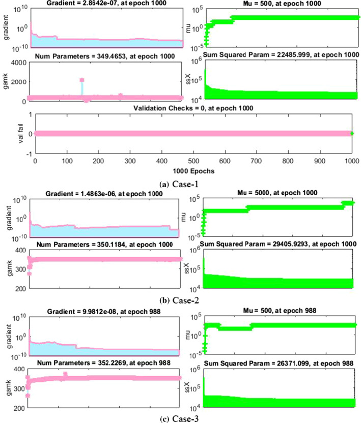
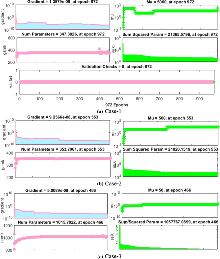
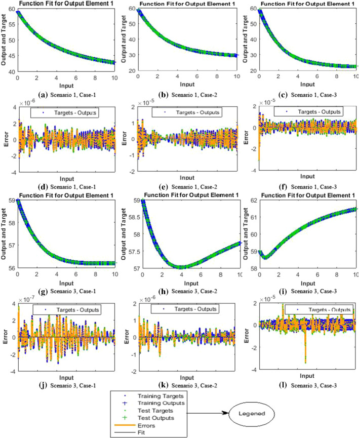
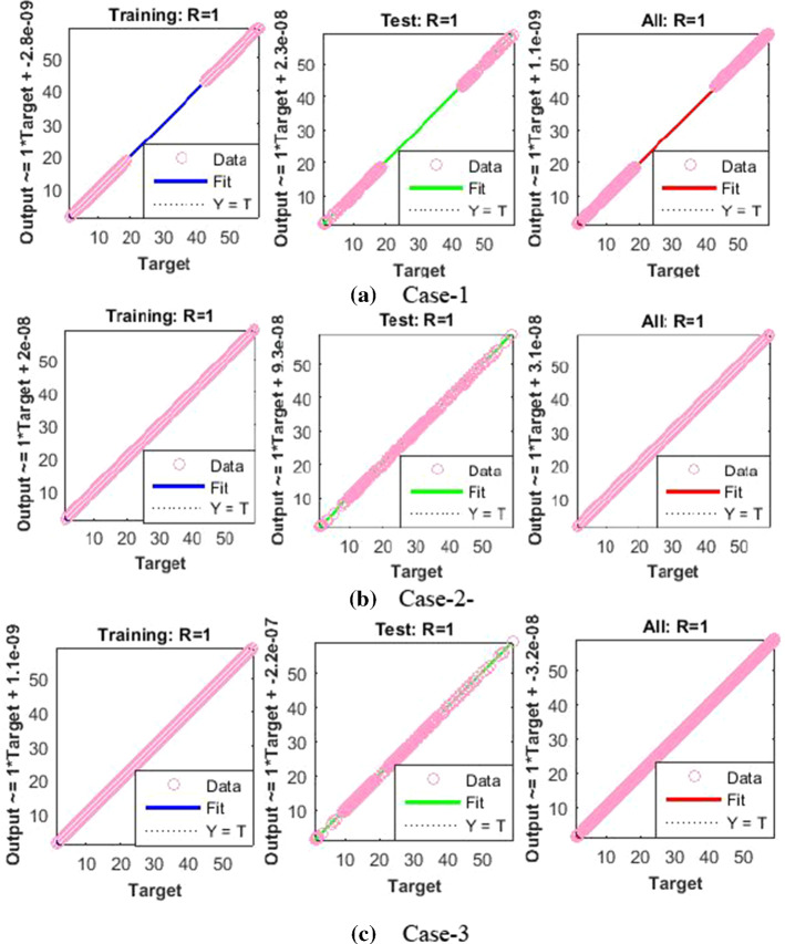
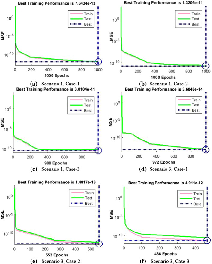
The results of NNs-BBRS for the nonlinear PVP-SD model based on the training states are graphically shows in Figs. 4 and 5, and the performance of fitness solution is shown in Fig. 6, while the regression curves are shown in Figs. 7 and 8 for scenarios 1 and 3, respectively, and the error histogram plots are shown in Fig. 9. Moreover, the results of mean squared error in terms of training, validation, testing, and performance, backpropagation indices, overall epochs and time for execution are provided in Table 3 for all cases of scenarios (1–4) of the nonlinear PVP-SD model by applying NNs-BBRS. By reviewing the time mentioned against each case, one can see the complexity of this scheme.

Fig. 4.

Training states of NNs-BBRS for the nonlinear PVP-SD model of scenario 1

Fig. 5.

Training states of NNs-BBRS for the nonlinear PVP-SD model of scenario 3

Fig. 6.

Fitness plots and error analysis of the nonlinear PVP-SD model

Fig. 7.

Regression curves of the nonlinear PVP-SD model for scenario 1

Fig. 8.

Regression curves of the nonlinear PVP-SD model for scenario 3

Fig. 9.

Error histogram of the nonlinear PVP-SD model for scenario 1 and scenario 3

Table 3.

Results of NNs-BBRS for the nonlinear PVP-SD model

Scenarios	Cases	MSE			Performance	Gradient	Mu	Epoch	Time (s)
		Training	Validation	Testing
1	1	7.64E–13	0.00E+00	9.01E–13	7.64E–13	2.86E–07	500	1000	< 199
	2	1.32E–11	0.00E+00	1.37E–11	1.32E–11	1.49E–06	5000	1000	< 211
	3	3.01E–11	0.00E+00	4.79E–11	3.01E–11	9.98E–08	500	988	< 206
2	1	1.56E–12	0.00E+00	1.98E–12	1.56E–12	6.88E–08	5000	646	< 131
	2	8.63E–14	0.00E+00	9.70E–14	8.63E–14	1.98E–08	5000	669	< 134
	3	4.50E–11	0.00E+00	6.99E–11	4.50E–11	1.13E–07	50	1000	< 103
3	1	3.60E–14	0.00E+00	4.81E–14	3.60E–14	1.36E–09	5000	972	< 194
	2	1.48E–13	0.00E+00	3.63E–13	1.48E–13	9.96E–08	500	553	< 108
	3	4.91E–12	0.00E+00	2.69E–11	4.91E–12	5.01E–09	50	466	< 557
4	1	6.24E–12	0.00E+00	7.84E–12	6.24E–12	6.24E–08	500	245	< 50
	2	3.69E–14	0.00E+00	5.50E–14	3.69E–14	1.10E–07	500	1000	< 104
	3	4.01E–12	0.00E+00	4.63E–12	4.01E–12	2.83E–08	500	448	< 89

The values of backpropagation indices Mu step size and gradient are [500, 5000, 500, 5000, 500, and 50] and [$2\text{.8642}\times {10}^{-07}$,$1.4863\times {10}^{-06}$, $9.9812\times {10}^{-08}$, $1.3579\times {10}^{-09}$, $9.9566\times {10}^{-08}$ and $5.0089\times {10}^{-09}$] as provided in Figs. 4a–c and 5a–c for all cases of scenarios 1 and 3, respectively.

The results endorsed the convergence and precision of the proposed scheme for every case of the nonlinear PVP-SD model. The performance of fitness solutions along with respective errors based on the training and testing samples is portrayed for every case of scenarios 1 and 3 for the nonlinear PVP-SD model in Fig. 6a–l. The competency of the proposed scheme can be observed by the overlapping of the NNs-BBRS solutions with Adams method results along with negligible errors. The regression analysis is measured by using co-relation studies, and plots are shown in Figs. 7a–c and 8a–c for every case of scenarios 1 and 3, respectively. The value of regression, R = 1, represents the rigorous linear relation between targets and outputs which endorsed the accurate working of proposed NNs-BBRS for training and testing samples.

The dynamics of error are additionally evaluated by histograms error for all inputs, and results are plotted in Fig. 9a–f, respectively, of the nonlinear PVP-SD model. The error bars bounded to the “0” error line have the accuracy level around $-8.5\times {10}^{-08}$, $-1.9\times {10}^{-06}$, $-9.8\times {10}^{-07}$, $1.81\times {10}^{-08}$, $2.05\times {10}^{-07}$ and $1.91\times {10}^{-06}$ indicating the best performance of the proposed NNs-BBRS. The convergence of the nonlinear PVP-SD model is further accessed in terms of MSE for the train and test samples and respective results are portrayed graphically in Fig. 10a–f for scenarios 1 and 3.

Fig. 10.

Performance of MSE for the nonlinear PVP-SD model

The results of NNs-BBRS are showing the best performance at epochs 1000, 1000, 988, 972, 553 and 466 with MSE around ${10}^{-13}$, ${10}^{-11}$, ${10}^{-11}$, ${10}^{-14}$, ${10}^{-13}$ and ${10}^{-12}$ for every case of scenarios 1 and 3, respectively.

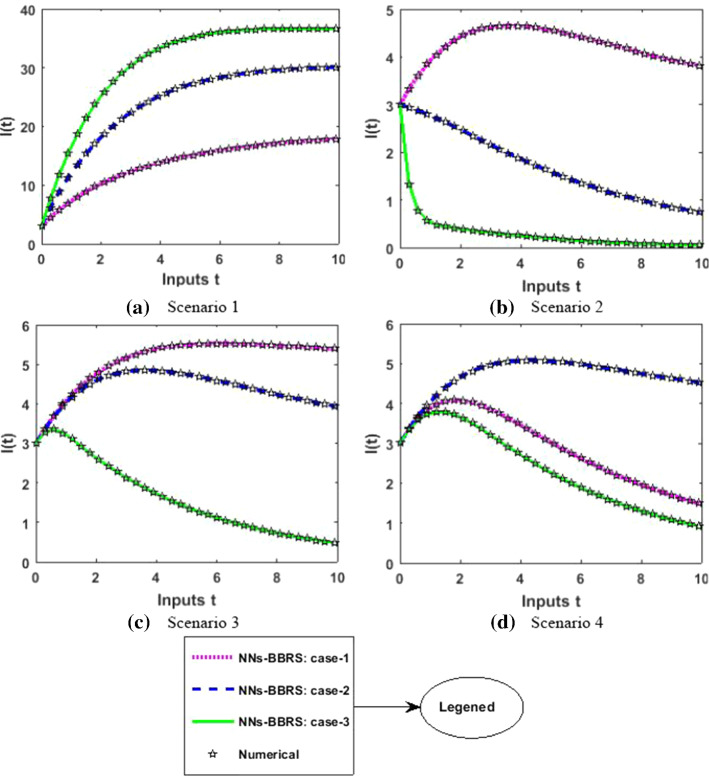
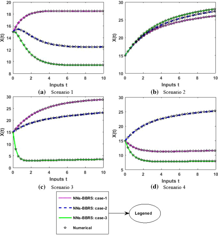
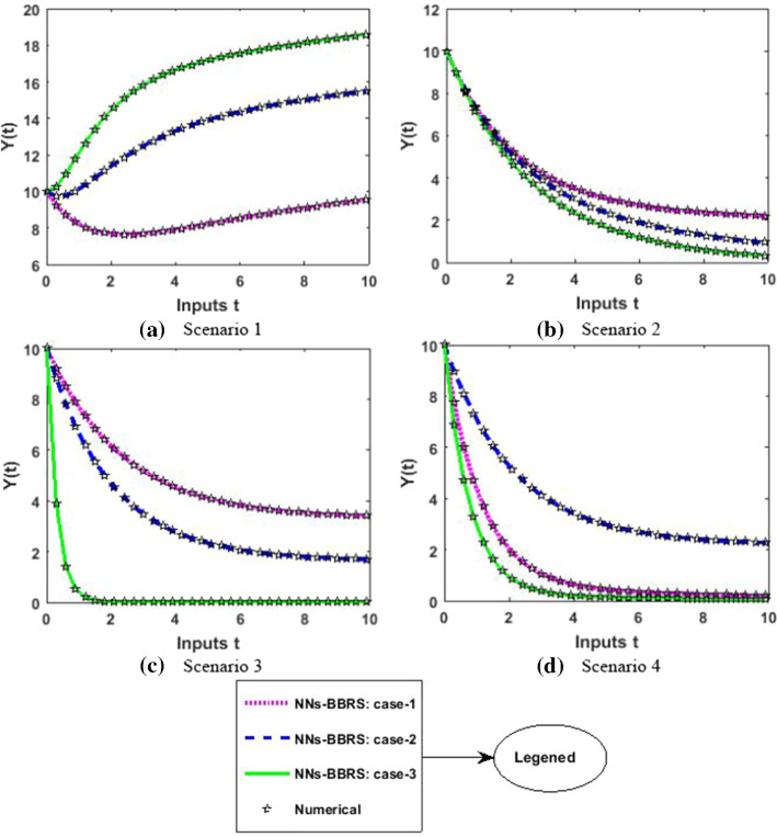
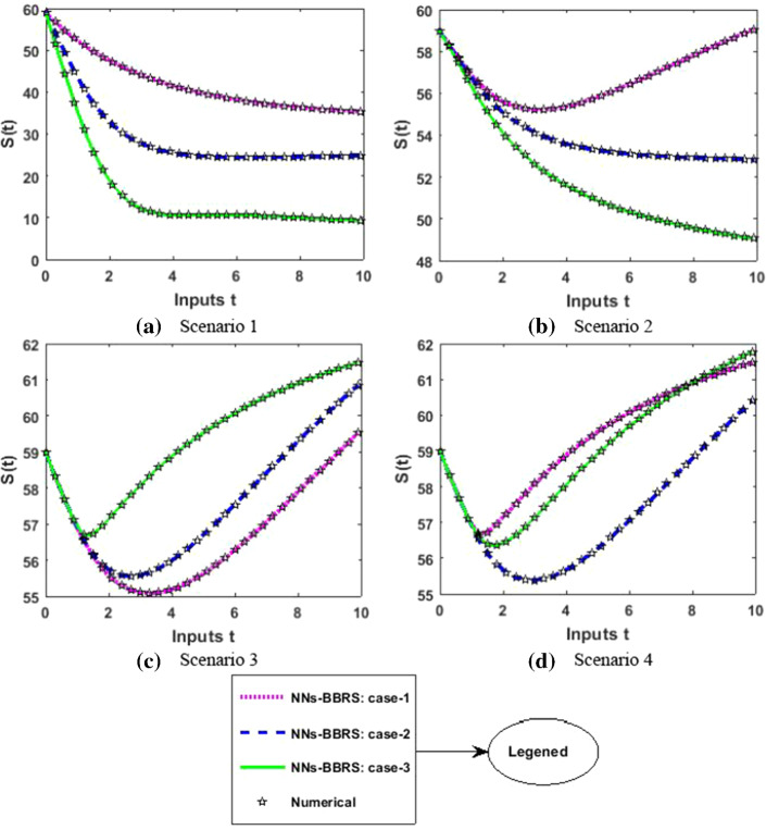
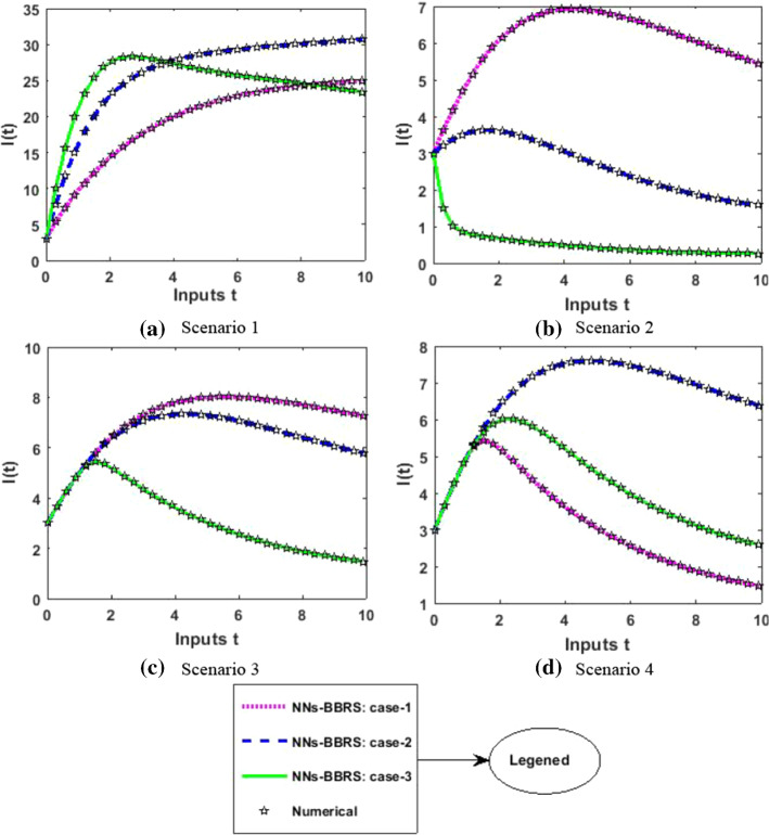
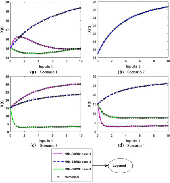
The approximate results for the S(t) susceptible class, I(t) infected class, X(t) susceptible insect vectors, Y(t) infected insect vectors and P(t) predators are determined by applying the NNs-BBRS for the variety of cases in the plant’s bite rate due to vectors, vector bite rate due to plants, plant’s recovery rate, predator contact rate with healthy insects, predator contact rate with infected insects and death rate caused by insecticides to describe the dynamics corresponding to 10 days for the nonlinear PVP-SD model. The performance of NNs-BBRS generated results are analyzed with Adams method reference results for every case of all the scenarios for the nonlinear PVP-SD model and results graphically shown in Figs. 11, 13, 15, 17 and 19. It is clearly seen from these subfigures the curves overlap each other which approves the accuracy of results for inputs 0 to 10 with step size 0.01.

Fig. 11.

Numerical results for S

Fig. 13.

Numerical results for I

Fig. 15.

Numerical results for X

Fig. 17.

Numerical results for Y

Fig. 19.

Numerical results for P

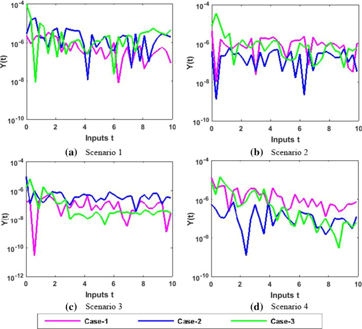
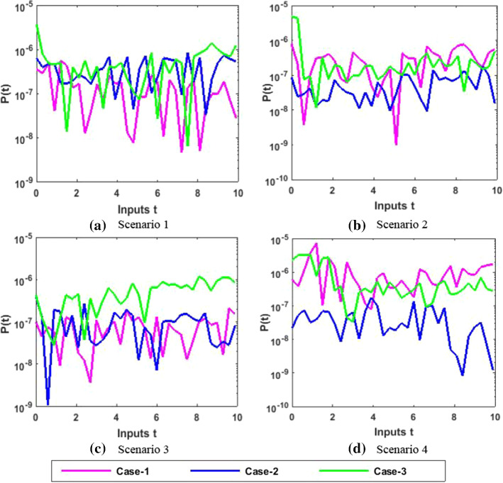
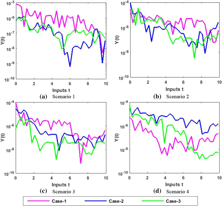
Therefore, the precision gauges of the designed NNs-BBRS are further accessed by calculating the absolute errors (AEs). The graphical representation of the results of AEs for all the five classes S(t), I(t), X(t), Y(t) and P(t) of the nonlinear PVP-SD model are portrayed, respectively, in Figs. 12, 14, 16, 18 and 20. The values of AEs for class S lie between ${10}^{-4}$ and ${10}^{-8}$, ${10}^{-4}$ and ${10}^{-10}$ for cases 1–3 of scenario 1 and 2, respectively, and ${10}^{-5}$ and ${10}^{-9}$ for cases 1–3 of scenario 3 and 4 as shown in Fig. 12a–d. The values of AEs for class I lie between ${10}^{-4}$ and ${10}^{-8}$, ${10}^{-4}$ and ${10}^{-10}$ for cases 1–3 of scenario 1 and 2, respectively, and ${10}^{-5}$ and ${10}^{-9}$, ${10}^{-5}$ and ${10}^{-10}$ for cases 1–3 of scenario 3 and 4, respectively, as presented in Fig. 14a–d. The values of AEs for class X lie between ${10}^{-4}$ and ${10}^{-8}$ for cases 1–3 of scenario 1 and 2, and ${10}^{-5}$ and ${10}^{-9}$, ${10}^{-5}$ and ${10}^{-8}$ for cases 1–3 of scenario 3 and 4, respectively, as portrayed in Fig. 16a–d. The values of AEs for class Y lie between ${10}^{-4}$ and ${10}^{-10}$ for cases 1–3 of scenario 1 and 2, and ${10}^{-4}$ and ${10}^{-12}$, ${10}^{-4}$ and ${10}^{-10}$ for cases 1–3 of scenario 3 and 4, respectively, as presented in Fig. 18a–d. The values of AEs for class P lie between ${10}^{-5}$ and ${10}^{-9}$ for cases 1–3 of scenario 1 and 3, and ${10}^{-5}$ and ${10}^{-10}$ for cases 1–3 of scenario 2 and 4 as presented in Fig. 19a–d. The competency of the results obtained by proposed NNs-BBRS can be notarized by overlapping the plots in all cases of the nonlinear PVP-SD model (Figs. 13, 14, 15, 16, 17, 18, 19, and 20).

Fig. 12.

Error analysis for S

Fig. 14.

Error Analysis for infected plants I

Fig. 16.

Error analysis for X

Fig. 18.

Error analysis for Y

Fig. 20.

Error analysis for P

Case study-II

Case study-II consists of the four scenarios which are constructed through the variety of cases by varying the plants bite rate due to vectors, vector bite rate due to plants, plant’s recovery rate, predator contact rate with healthy insects, predator contact rate with infected insects and death rate caused by insecticides as listed in Table 2 to examine the dynamics of the nonlinear PVP-SD model. The description and values of default parameters used for system (1) for all cases are tabulated in Table 1. Furthermore, the PVP-SD model has delays, ${\xi }_1=1$ and ${\xi }_2=24$, and seasonal impacts $\left(l=0.5\right)$.

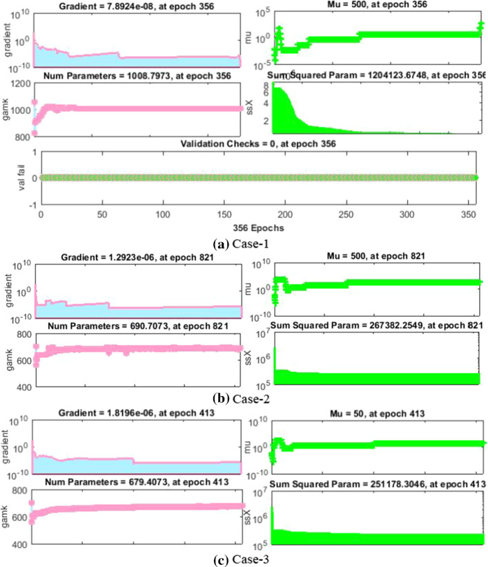
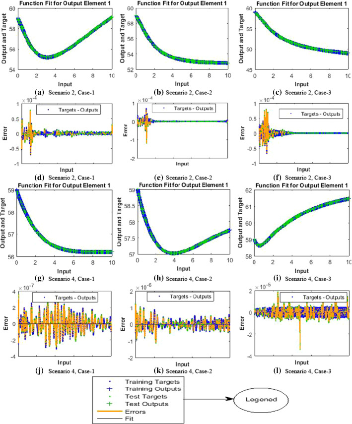
The results of NNs-BBRS for the nonlinear PVP-SD model in terms of training state are graphically presented in Figs. 21 and 22, and the performance of fitness solution is described in Fig. 23, while the regression curves are shown in Figs. 24 and 25, and plots of error histogram are shown in Fig. 26. In addition, the results of mean squared error in terms of training, validation, testing, and performance, backpropagation indices, overall epochs and time for execution are tabulated in Table 4 for all cases of scenarios (1–4) of the nonlinear PVP-SD model by applying NNs-BBRS. The intricacy of the proposed scheme can be observed by the time mentioned against each case for all the scenarios of the nonlinear PVP-SD model.

Fig. 21.

Training states of NNs-BBRS for the nonlinear PVP-SD model of scenario 2

Fig. 22.

Training states of NNs-BBRS for the nonlinear PVP-SD model of scenario 4

Fig. 23.

Fitness plots and error dynamics of the nonlinear PVP-SD model

Fig. 24.

Regression curves of the nonlinear PVP-SD model for scenario 2

Fig. 25.

Regression curves of the nonlinear PVP-SD model for scenario 4

Fig. 26.

Error histogram of the nonlinear PVP-SD model for scenario 2 and 4

Table 4.

Results of NNs-BBRS for the nonlinear PVP-SD model

Scenarios	Cases	MSE			Performance	Gradient	Mu	Epoch	Time (s)
		Training	Validation	Testing
1	1	1.88E–11	0.00E+00	6.17E–11	1.88E–11	9.96E–08	50	492	< 493
	2	2.76E–11	0.00E+00	7.17E–11	2.76E–11	3.38E–06	500	682	< 707
	3	3.30E–11	0.00E+00	9.65E–11	3.30E–11	9.40E–07	50	199	< 346
2	1	3.62E–11	0.00E+00	5.55E–11	3.62E–11	6.23E–07	500	464	< 74
	2	3.33E–11	0.00E+00	1.50E–11	3.33E–11	6.73E–08	50,000	42	< 42
	3	7.04E–11	0.00E+00	1.44E–10	7.04E–11	8.59E–08	500	173	< 122
3	1	2.70E–11	0.00E+00	8.42E–11	2.70E–11	1.15E–06	500	1000	< 361
	2	3.40E–11	0.00E+00	2.92E–11	3.40E–11	9.58E–08	500	42	< 26
	3	2.07E–11	0.00E+00	5.18E–11	2.07E–11	7.25E–07	5	287	< 313
4	1	2.18E–11	0.00E+00	8.27E–11	2.18E–11	7.89E–08	500	356	< 427
	2	4.82E–11	0.00E+00	9.33E–11	4.82E–11	1.29E–06	500	821	< 626
	3	1.58E–11	0.00E+00	3.83E–11	1.58E–11	1.82E–06	50	413	< 308

The values of backpropagation indices Mu step size and gradient are [500, 50,000, 500, 500, 500 and 50] and [$6\text{.2345}\times {10}^{-07}$,$6.7348\times {10}^{-08}$, $8.5943\times {10}^{-08}$, $7.8924\times {10}^{-08}$, $1.2923\times {10}^{-06}$ and $1.8196\times {10}^{-06}$] as provided in Figs. 21a–c and 22a–c for all cases of scenarios 2 and 4, respectively. The results endorsed the convergence and precision of the proposed scheme for every case of the nonlinear PVP-SD model. The performance of fitness solutions and respective error dynamics based on the training and testing samples is portrayed for every case of scenarios 2 and 4 for the nonlinear PVP-SD model in Fig. 23a–l. It is envisioned from these subfigures that the NNs-BBRS generated outcomes, and the referenced Adams results overlap each other with small amount of errors which proves the accuracy of the results.

Co-relation studies are consumed for regression analysis, and the corresponding results are portrayed graphically in Figs. 24a–c and 25a–c for each case of scenarios 2 and 4 of the nonlinear PVP-SD model. The rigorous linear relation between targets and output values can be found for the value of regression, R = 1, in these subfigures which verified the accurate working of training and testing samples of the proposed NNs-BBRS for the nonlinear PVP-SD model.

The dynamics of error are further determined by histogram error for all input points and corresponding results are portrayed graphically in Fig. 26a–f for each case of scenario 2 and 4 of the nonlinear PVP-SD model, respectively. The best performance of the proposed NNs-BBRS is indicated by the boundedness of error bars to the “0” error line as shown in subfigures, and the level of accuracy lies in $-1.5\times {10}^{-07}$, $9.73\times {10}^{-07}$, $-4.4\times {10}^{-06}$, $-7.4\times {10}^{-06}$, $-6.98\times {10}^{-08}$ and $2.85\times {10}^{-06}$ for cases 1–3 of scenarios 2 and 4, respectively. The results of MSE for the train and test samples are calculated to approve the convergence of the nonlinear PVP-SD model, and plots of respective results are provided in Fig. 27a–f for scenarios 2 and 4. The best performance of NNs-BBRS is obtained at epochs 464, 42, 173, 356, 821, and 413 with MSE around ${10}^{-11}$ for every case of scenarios 2 and 4, respectively, for the nonlinear PVP-SD model.

Fig. 27.

Performance of MSE for the nonlinear PVP-SD model

The performance of the proposed NNs-BBRS generated results is examined with Adam’s method reference results for every case of all the scenarios of the nonlinear PVP-SD model, and graphical representation is presented in Figs. 28, 30, 32, 34 and 36. The curves overlap each other which approves the accuracy of results for inputs 0 to 10 with step size 0.01.

Fig. 28.

Numerical results for S

Fig. 30.

Numerical results for I

Fig. 32.

Numerical results for X

Fig. 34.

Numerical results for Y

Fig. 36.

Numerical results for P

Therefore, the approximate results are determined by applying the NNs-BBRS for the S(t) susceptible class, I(t) infected class, R(t) recovered class, X(t) susceptible insect vectors, Y(t) infected insect vectors and P(t) predators for the variety of cases in the plant’s bite rate due to vectors, vector bite rate due to plants, plant’s recovery rate, predator contact rate with healthy insects, predator contact rate with infected insects and death rate caused by insecticides to describe the dynamics corresponding to 10 days of the nonlinear PVP-SD model. The comparison of the approximate results of NNs-BBRS and reference results of Adams method are graphically portrayed in Figs. 28, 30, 32, 34 and 36. The convergence of the proposed NNs-BBRS can be noticed through the overlapping of the plots for each case of all the scenarios of the nonlinear PVP-SD model.

Therefore, the AEs of the designed NNs-BBRS generated outcomes are also calculated in order to validate the precision gauges. The graphical representation of the results of AEs for all the five classes S(t), I(t), X(t), Y(t) and P(t) of the nonlinear PVP-SD model is portrayed, respectively in Figs. 29, 31, 33, 35 and 37. The values of AEs for class S lie between ${10}^{-4}$ and ${10}^{-10}$ for cases 1–3 of scenarios 1, 2 and 4, and ${10}^{-4}$ and ${10}^{-8}$ for cases 1–3 of scenarios 3 as shown in Fig. 29a–d. The values of AEs for class I lie between ${10}^{-4}$ and ${10}^{-8}$ for cases 1–3 of scenarios 1 and 4, and ${10}^{-2}$ and ${10}^{-10}$, ${10}^{-4}$ and ${10}^{-10}$ for cases 1–3 of scenarios 2 and 3, respectively as presented in Fig. 31a–d. The values of AEs for class X lie between ${10}^{-4}$ and ${10}^{-10}$ for cases 1–3 of scenarios 1 and 4, and ${10}^{-2}$ and ${10}^{-10}$, ${10}^{-2}$ to ${10}^{-8}$ for cases 1–3 of scenarios 2 and 3, respectively, as portrayed in Fig. 33a–d. The values of AEs for class Y lie between ${10}^{-5}$ and ${10}^{-10}$ for cases 1–3 of scenario 1, and ${10}^{-4}$ and ${10}^{-10}$ for cases 1–3 of scenarios 2, 3 and 4 as presented in Fig. 35a–d. The values of AEs for class P lie between ${10}^{-5}$ and ${10}^{-9}$ for cases 1–3 of scenarios 1 and 3, and ${10}^{-5}$ and ${10}^{-10}$ for cases 1–3 of scenario 2 and 4 as presented in Fig. 37a–d. The competency of the results obtained by proposed NNs-BBRS can be notarized by overlapping the plots in all cases of the nonlinear PVP-SD model (Figs. 30, 31, 32, 33, 34, 35, 36, and 37).

Fig. 29.

Error analysis for S

Fig. 31.

Error analysis for I

Fig. 33.

Error analysis for X

Fig. 35.

Error analysis for Y

Fig. 37.

Error analysis for P

Conclusion

A stochastic paradigm based on an artificial intelligence is introduced by employing the knacks of neural networks as well as backpropagation of Bayesian regularization scheme for solving the mathematical model for plant virus propagation with the impact of seasonality and delays representing the dynamical behavior of plants bite rate due to vectors, vector bite rate due to plants, plant’s recovery rate, predator contact rate with healthy insects, predator contact rate with infected insects and death rate caused by insecticides. The reference dataset are generated with the help of Adams method for all five classes of the nonlinear PVP-SD model. The dataset for the nonlinear PVP-SD model is arbitrarily used as 75%, 5% and 10% for the training, validation and testing samples for the NNs-BBRS, respectively. Following are the remarkable ascertainments of the mathematical model for PVP-SD model based on the foregoing numerical simulation and analysis.

• The design stochastic paradigm NNs-BBRS is used effectively to find the approximate solution of the governing ODEs system representing the nonlinear PVP-SD model.

• The precision and convergence of the proposed NNs-BBRS are effectively examined by comparative studies of the referenced numerical solutions procured by the Adams method and the results of MSE lie approximately in ${10}^{-12}$ to ${10}^{-14}$ and ${10}^{-11}$ for the variety of cases of different scenarios for case study-I and case study-II, respectively, that illustrate the best performance of testing, training as well as validation samples.

• The designed NNs-BBRS is robust, efficient and stable computing platform as investigated by the illustrations of histogram errors, regression matrices and MSE learning curves by the execution of exhaustive simulations.

In future, one exploit such AI-based heuristic computing architectures to broad field of applied science and technology [82–93].

List of symbols

PVP-SD

Plant virus propagation with impact of the seasonality and delays

NNs

Neural networks

NNs-BBRS

Neural networks backpropagation with Bayesian regularization scheme

AI

Artificial intelligence

ANNs

Artificial neural networks

COVID-19

Corona virus disease 2019

S, I, X, Y and P

Susceptible, infected, exposed and recovered

S₀, I₀, X₀, Y₀ and P₀

Initial values of S, I, X, Y and P

HIV

Human immunodeficiency virus

TLCD

Tobacco leaf curl disease

SIR

Susceptible, infected and recovered

NDSolve

Numerical solution of differential equations

MSE

Mean square error

AEs

Absolute errors

$N$

Population of plant hosts

$\alpha$

Plants bite rate due to vectors

${\alpha }_1$

Vector bite rate due to plants

$\gamma$

Plant saturation constant due to vectors

${\gamma }_1$

Vector saturation constant due to plants

$\upsilon$

Plant’s natural death rate

$k$

Vector’s natural death rate

$\beta$

Plant’s recovery rate

$\mathrm{\Lambda }$

Vectors replenishing rate

$c$

Infected plants death rate due to the disease

$d_1$

Predator contact rate with healthy insects

$d_2$

Rate of contact between predators and infected insects

$\eta$

Rate of natural death of predators

$\delta$

Constant competition between predators

${\gamma }_3$

Predators' saturation caused by insects

${\gamma }_4$

Predator conversion rate due to insects

$c_{\text{in}}$

Death rate caused by insecticides

${\mathrm{\Lambda }}_{\text{p}}$

Addition rate of predators

Data availability statement

There is no any data associated with this article.

Declarations

Conflict of interest

All the authors of the article declared that there is no any conflict of interest.

References

- 1.Uke A, Tokunaga H, Utsumi Y, Vu NA, Nhan PT, Srean P, Hy NH, Lopez-Lavalle LAB, Ishitani M, Hung N, Van Hong N. Cassava mosaic disease and its management in Southeast Asia. Plant Mol. Biol. 2021;9:1–11. doi: 10.1007/s11103-021-01168-2. [DOI] [PMC free article] [PubMed] [Google Scholar]
- 2.Sharma N, Prasad M. Silencing AC1 of Tomato leaf curl virus using artificial microRNA confers resistance to leaf curl disease in transgenic tomato. Plant Cell Rep. 2020;39(11):1565–1579. doi: 10.1007/s00299-020-02584-2. [DOI] [PubMed] [Google Scholar]
- 3.B.L. Patil, Plant viral diseases: Economic implications. In: Encyclopedia of Virology, 4th edition. Edited by D. Bamford & M. Zuckerman; Elsevier Limited. Chapter 21307. 10.1016/B978-0-12-809633-8.21307-1 (2020)
- 4.M. Sarwar, Insects as transport devices of plant viruses. In Applied Plant Virology (Academic Press, 2020), pp. 381–402
- 5.Rossi V, Sperandio G, Caffi T, Simonetto A, Gilioli G. Critical success factors for the adoption of decision tools in IPM. Agronomy. 2019;9(11):710. doi: 10.3390/agronomy9110710. [DOI] [Google Scholar]
- 6.Shelton AM, Long SJ, Walker AS, Bolton M, Collins HL, Revuelta L, Johnson LM, Morrison NI. First field release of a genetically engineered, self-limiting agricultural pest insect: evaluating its potential for future crop protection. Front. Bioeng. Biotechnol. 2020;7:482. doi: 10.3389/fbioe.2019.00482. [DOI] [PMC free article] [PubMed] [Google Scholar]
- 7.Chowdhury J, Al Basir F, Takeuchi Y, Ghosh M, Roy PK. A mathematical model for pest management in Jatropha curcas with integrated pesticides—an optimal control approach. Ecol. Complex. 2019;37:24–31. doi: 10.1016/j.ecocom.2018.12.004. [DOI] [Google Scholar]
- 8.N.P. Pratiwi, D. Aldila, B.D. Handari, G.M. Simorangkir, A mathematical model to control Mosaic disease of Jatropha curcas with insecticide and nutrition intervention. In AIP Conference Proceedings, vol. 2296, No. 1 (AIP Publishing LLC, 2020), p. 020096
- 9.Liu S, Huang M, Wang J. Bifurcation control of a delayed fractional Mosaic disease model for Jatropha curcas with farming awareness. Complexity. 2020;2020:1–16. [Google Scholar]
- 10.Al Basir F, Ray S. Impact of farming awareness based roguing, insecticide spraying and optimal control on the dynamics of mosaic disease. Ricerche Mat. 2020;69:393–412. doi: 10.1007/s11587-020-00522-8. [DOI] [Google Scholar]
- 11.Wei X, Wang L, Jia Q, Xiao J, Zhu G. Assessing different interventions against Avian Influenza A (H7N9) infection by an epidemiological model. One Health. 2021;13:100312. doi: 10.1016/j.onehlt.2021.100312. [DOI] [PMC free article] [PubMed] [Google Scholar]
- 12.C. Ratchford, Multi-scale and multi-group modeling techniques applied to Cholera and COVID-19 (2021)
- 13.N.K.O. Opoku, C. Afriyie, The role of control measures and the environment in the transmission dynamics of cholera. In Abstract and Applied Analysis, vol. 2020 (Hindawi, 2020)
- 14.S.E. Moore, E. Okyere, Controlling the transmission dynamics of COVID-19. arXiv preprint arXiv: 2004.00443 (2020)
- 15.Shi F, Yu C, Yang L, Li F, Lun J, Gao W, Xu Y, Xiao Y, Shankara SB, Zheng Q, Zhang B. Exploring the dynamics of hemorrhagic fever with renal syndrome incidence in East China through seasonal autoregressive integrated moving average models. Infect. Drug Resist. 2020;13:2465. doi: 10.2147/IDR.S250038. [DOI] [PMC free article] [PubMed] [Google Scholar]
- 16.Jiang X, Chen X, Chi M, Chen J. On Hopf bifurcation and control for a delay systems. Appl. Math. Comput. 2020;370:124906. [Google Scholar]
- 17.Alemneh HT, Kassa AS, Godana AA. An optimal control model with cost effectiveness analysis of Maize streak virus disease in maize plant. Infect. Dis. Model. 2021;6:169–182. doi: 10.1016/j.idm.2020.12.001. [DOI] [PMC free article] [PubMed] [Google Scholar]
- 18.Doussoulin JP. A paradigm of the circular economy: the end of cheap nature? Energy, Ecol. Environ. 2020;5(5):359–368. doi: 10.1007/s40974-019-00145-2. [DOI] [Google Scholar]
- 19.Gazi NH, Biswas SK. Holling–Tanner predator-prey model with type-IV functional response and harvesting. Discontin., Nonlinearity, Complex. 2021;10(01):151–159. doi: 10.5890/DNC.2021.03.011. [DOI] [Google Scholar]
- 20.R. Wu, Permanence of a nonlinear mutualism model with time varying delay (2019)
- 21.Jiang X, Chen X, Huang T, Yan H. Bifurcation and control for a predator-prey system with two delays. IEEE Trans. Circuits Syst. II Express Briefs. 2020;68(1):376–380. [Google Scholar]
- 22.Mondal S, Samanta GP. Dynamical behaviour of a two-prey and one-predator system with help and time delay. Energy, Ecol. Environ. 2020;5(1):12–33. doi: 10.1007/s40974-019-00141-6. [DOI] [Google Scholar]
- 23.Wu LQ, Wang XY. Qualitative analysis of a four-dimensional predator-prey model with two delays. J. North Univ. China (Nat. Sci. Edit.) 2019;2019:02. [Google Scholar]
- 24.Wang C, Jia L, Li L, Wei W. Global stability in a delayed ratio-dependent predator-prey system with feedback controls. IAENG Int. J. Appl. Math. 2020;50(3):1–9. [Google Scholar]
- 25.Roy J, Barman D, Alam S. Role of fear in a predator-prey system with ratio-dependent functional response in deterministic and stochastic environment. Biosystems. 2020;197:104176. doi: 10.1016/j.biosystems.2020.104176. [DOI] [PubMed] [Google Scholar]
- 26.Zheng W, Sugie J. Uniform global asymptotic stability of time-varying Lotka–Volterra predator–prey systems. Appl. Math. Lett. 2019;87:125–133. doi: 10.1016/j.aml.2018.07.030. [DOI] [Google Scholar]
- 27.Ray S, Al Basir F. Impact of incubation delay in plant–vector interaction. Math. Comput. Simul. 2020;170:16–31. doi: 10.1016/j.matcom.2019.09.001. [DOI] [Google Scholar]
- 28.Wang Z, Liu L, Su G, Shao Y. On an impulsive food web system with mutual interference and distributed time delay. Discret. Dyn. Nat. Soc. 2020;2020:1–21. doi: 10.1155/2020/6689089. [DOI] [Google Scholar]
- 29.Zhang Y, Li L, Huang J, Liu Y. Stability and Hopf bifurcation analysis of a vector-borne disease model with two delays and reinfection. Comput. Math. Methods Med. 2021;2021:1895764. doi: 10.1155/2021/1895764. [DOI] [PMC free article] [PubMed] [Google Scholar] [Retracted]
- 30.Darti I, Suryanto A, Hartono M. Global stability of a discrete SIR epidemic model with saturated incidence rate and death induced by the disease. Commun. Math. Biol. Neurosci. 2020;2020:33. [Google Scholar]
- 31.Zhang Z, Zou J, Upadhyay RK, Pratap A. Stability and Hopf bifurcation analysis of a delayed tobacco smoking model containing snuffing class. Adv. Differ. Equ. 2020;2020(1):1–19. doi: 10.1186/s13662-019-2438-0. [DOI] [PMC free article] [PubMed] [Google Scholar]
- 32.Alcaide C, Rabadán MP, Moreno-Perez MG, Gómez P. Implications of mixed viral infections on plant disease ecology and evolution. Adv. Virus Res. 2020;106:145–169. doi: 10.1016/bs.aivir.2020.02.001. [DOI] [PubMed] [Google Scholar]
- 33.Chen-Charpentier B. Stochastic modeling of plant virus propagation with biological control. Mathematics. 2021;9(5):456. doi: 10.3390/math9050456. [DOI] [Google Scholar]
- 34.M. Chapwanya, Y. Dumont, Application of mathematical epidemiology to crop vector-borne diseases: the Cassava Mosaic virus disease case. In Infectious Diseases and Our Planet (Springer, Cham, 2021), pp. 57–95
- 35.Al Basir F, Kyrychko YN, Blyuss KB, Ray S. Effects of vector maturation time on the dynamics of Cassava Mosaic disease. Bull. Math. Biol. 2021;83(8):1–21. doi: 10.1007/s11538-021-00921-4. [DOI] [PMC free article] [PubMed] [Google Scholar]
- 36.Zhong W, Murad MAA, Liu M, Milano F. Impact of virtual power plants on power system short-term transient response. Electric Power Syst. Res. 2020;189:106609. doi: 10.1016/j.epsr.2020.106609. [DOI] [Google Scholar]
- 37.Waezizadeh T, Parsaei T, Fourozesh F. Dynamical model for virus transmission in plants with two time delays. Math. Res. 2020;6(3):487–500. [Google Scholar]
- 38.Mukherjee D. Effect of constant immigration in plant–pathogen–herbivore interactions. Math. Comput. Simul. 2019;160:192–200. doi: 10.1016/j.matcom.2018.12.015. [DOI] [Google Scholar]
- 39.Fei L, Zou L, Chen X. Global analysis for an epidemical model of vector-borne plant viruses with disease resistance and nonlinear incidence. J. Appl. Anal. Comput. 2020;10(5):2085–2103. [Google Scholar]
- 40.Luo Y, Gao S, Xie D, Dai Y. A discrete plant disease model with roguing and replanting. Adv. Differ. Equ. 2015;2015(1):1–18. doi: 10.1186/s13662-014-0332-3. [DOI] [Google Scholar]
- 41.Misra OP, Babu AR. Modelling effect of toxicant in a three-species food-chain system incorporating delay in toxicant uptake process by prey. Model. Earth Syst. Environ. 2016;2(2):77. doi: 10.1007/s40808-016-0128-4. [DOI] [Google Scholar]
- 42.Getz WM, Salter R, Mgbara W. Adequacy of SEIR models when epidemics have spatial structure: Ebola in Sierra Leone. Philos. Trans. R. Soc. B. 2019;374(1775):20180282. doi: 10.1098/rstb.2018.0282. [DOI] [PMC free article] [PubMed] [Google Scholar]
- 43.Too EC, Yujian L, Njuki S, Yingchun L. A comparative study of fine-tuning deep learning models for plant disease identification. Comput. Electron. Agric. 2019;161:272–279. doi: 10.1016/j.compag.2018.03.032. [DOI] [Google Scholar]
- 44.O. Chase, I. Ferriol, J.J. López-Moya, Control of plant pathogenic viruses through interference with insect transmission. In Plant Virus-Host Interaction (Academic Press, 2021), pp. 359–381
- 45.Wu JY, Zhang Y, Zhou XP, Qian YJ. Three sensitive and reliable serological assays for detection of potato virus A in potato plants. J. Integr. Agric. 2021;20(11):2966–2975. doi: 10.1016/S2095-3119(20)63492-X. [DOI] [Google Scholar]
- 46.Swain S, Nayak SK, Barik SS. A review on plant leaf diseases detection and classification based on machine learning models. Mukt shabd. 2020;9(6):5195–5205. [Google Scholar]
- 47.Chen-Charpentier BM, Jackson M. Direct and indirect optimal control applied to plant virus propagation with seasonality and delays. J. Comput. Appl. Math. 2020;380:112983. doi: 10.1016/j.cam.2020.112983. [DOI] [Google Scholar]
- 48.Abdullah Z, et al. Design of wideband tonpilz transducers for underwater SONAR applications with finite element model. Appl. Acoust. 2021;183:108293. doi: 10.1016/j.apacoust.2021.108293. [DOI] [Google Scholar]
- 49.Shoaib M, et al. Intelligent computing Levenberg Marquardt approach for entropy optimized single-phase comparative study of second grade nanofluidic system. Int. Commun. Heat Mass Transf. 2021;127:105544. doi: 10.1016/j.icheatmasstransfer.2021.105544. [DOI] [Google Scholar]
- 50.Awais M, et al. Intelligent numerical computing paradigm for heat transfer effects in a Bodewadt flow. Surf. Interfaces. 2021;26:101321. doi: 10.1016/j.surfin.2021.101321. [DOI] [Google Scholar]
- 51.Raja MAZ, Manzar MA, Shah SM, Chen Y. Integrated intelligence of fractional neural networks and sequential quadratic programming for Bagley-Torvik systems arising in fluid mechanics. J. Comput. Nonlinear Dyn. 2020;15(5):051003. doi: 10.1115/1.4046496. [DOI] [Google Scholar]
- 52.Bukhari AH, et al. Neuro-fuzzy modeling and prediction of summer precipitation with application to different meteorological stations. Alex. Eng. J. 2020;59(1):101–116. doi: 10.1016/j.aej.2019.12.011. [DOI] [Google Scholar]
- 53.Uddin I, Ullah I, et al. The intelligent networks for double-diffusion and MHD analysis of thin film flow over a stretched surface. Sci. Rep. 2021;11(1):1–20. doi: 10.1038/s41598-021-97458-2. [DOI] [PMC free article] [PubMed] [Google Scholar]
- 54.Ahmad I, et al. Stochastic numerical computing with Levenberg-Marquardt backpropagation for performance analysis of heat sink of functionally graded material of the porous fin. Surf. Interfaces. 2021;26:101403. doi: 10.1016/j.surfin.2021.101403. [DOI] [Google Scholar]
- 55.Mehmood A, et al. Integrated computational intelligent paradigm for nonlinear electric circuit models using neural networks, genetic algorithms and sequential quadratic programming. Neural Comput. Appl. 2020;32(14):10337–10357. doi: 10.1007/s00521-019-04573-3. [DOI] [Google Scholar]
- 56.Ali S, et al. Analysis of Williamson nanofluid with velocity and thermal slips past over a stretching sheet by Lobatto IIIA numerically. Therm. Sci. 2021;25:159. doi: 10.2298/TSCI200620159A. [DOI] [Google Scholar]
- 57.Khan I, et al. Design of neural network with Levenberg-Marquardt and Bayesian regularization backpropagation for solving pantograph delay differential equations. IEEE Access. 2020;8:137918–137933. doi: 10.1109/ACCESS.2020.3011820. [DOI] [Google Scholar]
- 58.Chaudhary NI, et al. Design of multi innovation fractional LMS algorithm for parameter estimation of input nonlinear control autoregressive systems. Appl. Math. Model. 2021;93:412–425. doi: 10.1016/j.apm.2020.12.035. [DOI] [Google Scholar]
- 59.Raja MAZ, et al. Intelligent computing for the dynamics of entropy optimized nanofluidic system under impacts of MHD along thick surface. Int. J. Mod. Phys. B. 2021;35:2150269. doi: 10.1142/S0217979221502696. [DOI] [Google Scholar]
- 60.Khan BS, et al. Design of moth flame optimization heuristics for integrated power plant system containing stochastic wind. Appl. Soft Comput. 2021;104:107193. doi: 10.1016/j.asoc.2021.107193. [DOI] [Google Scholar]
- 61.Almalki MM, et al. Optimization through the Levenberg–Marquardt backpropagation method for a magnetohydrodynamic squeezing flow system. Coatings. 2021;11(7):779. doi: 10.3390/coatings11070779. [DOI] [Google Scholar]
- 62.Bukhari AH, et al. Fractional neuro-sequential ARFIMA-LSTM for financial market forecasting. IEEE Access. 2020;8:71326–71338. doi: 10.1109/ACCESS.2020.2985763. [DOI] [Google Scholar]
- 63.Ahmad SI, et al. A new heuristic computational solver for nonlinear singular Thomas-Fermi system using evolutionary optimized cubic splines. Eur. Phys. J. Plus. 2020;135(1):1–29. doi: 10.1140/epjp/s13360-019-00066-3. [DOI] [Google Scholar]
- 64.Zaman F, et al. Novel computational heuristics for wireless parameters estimation in bistatic radar systems. Wirel. Pers. Commun. 2020;111(2):909–927. doi: 10.1007/s11277-019-06892-z. [DOI] [Google Scholar]
- 65.Bukhari AH, et al. Design of a hybrid NAR-RBFs neural network for nonlinear dusty plasma system. Alex. Eng. J. 2020;59(5):3325–3345. doi: 10.1016/j.aej.2020.04.051. [DOI] [Google Scholar]
- 66.Awan SE, et al. Numerical treatments to analyze the nonlinear radiative heat transfer in MHD nanofluid flow with solar energy. Arab. J. Sci. Eng. 2020;45(6):4975–4994. doi: 10.1007/s13369-020-04593-5. [DOI] [Google Scholar]
- 67.Umar M, et al. Stochastic numerical technique for solving HIV infection model of CD4+ T cells. Eur. Phys. J. Plus. 2020;135(5):403. doi: 10.1140/epjp/s13360-020-00417-5. [DOI] [Google Scholar]
- 68.Ahmad I, et al. Integrated neuro-evolution-based computing solver for dynamics of nonlinear corneal shape model numerically. Neural Comput. Appl. 2020;33:1–17. [Google Scholar]
- 69.Raja MAZ, Shah FH, Alaidarous ES, Syam MI. Design of bio-inspired heuristic technique integrated with interior-point algorithm to analyze the dynamics of heartbeat model. Appl. Soft Comput. 2017;52:605–629. doi: 10.1016/j.asoc.2016.10.009. [DOI] [Google Scholar]
- 70.Cheema TN, et al. Intelligent computing with Levenberg–Marquardt artificial neural networks for nonlinear system of COVID-19 epidemic model for future generation disease control. Eur. Phys. J. Plus. 2020;135(11):1–35. doi: 10.1140/epjp/s13360-020-00910-x. [DOI] [PMC free article] [PubMed] [Google Scholar]
- 71.Umar M, et al. A stochastic intelligent computing with neuro-evolution heuristics for nonlinear SITR system of novel COVID-19 dynamics. Symmetry. 2020;12(10):1628. doi: 10.3390/sym12101628. [DOI] [Google Scholar]
- 72.Umar M, et al. A stochastic computational intelligent solver for numerical treatment of mosquito dispersal model in a heterogeneous environment. Eur. Phys. J. Plus. 2020;135(7):1–23. doi: 10.1140/epjp/s13360-020-00557-8. [DOI] [Google Scholar]
- 73.Khan AA, et al. Fractional LMS and NLMS algorithms for line echo cancellation. Arab. J. Sci. Eng. 2021;2018:1–14. [Google Scholar]
- 74.Muhammad Y, et al. Design of fractional evolutionary processing for reactive power planning with FACTS devices. Sci. Rep. 2021;11(1):1–29. doi: 10.1038/s41598-020-79838-2. [DOI] [PMC free article] [PubMed] [Google Scholar]
- 75.Masood Z, et al. Fractional dynamics of stuxnet virus propagation in industrial control systems. Mathematics. 2021;9(17):2160. doi: 10.3390/math9172160. [DOI] [Google Scholar]
- 76.Khan MW, et al. A new fractional particle swarm optimization with entropy diversity based velocity for reactive power planning. Entropy. 2020;22(10):1112. doi: 10.3390/e22101112. [DOI] [PMC free article] [PubMed] [Google Scholar]
- 77.Stella IR, Srivastav AK, Ghosh M. Modeling and analysis of vector-borne plant disease with two delays. J. Phys.: Conf. Ser. 2021;1850(1):012125. [Google Scholar]
- 78.Jackson M, Chen-Charpentier BM. A model of biological control of plant virus propagation with delays. J. Comput. Appl. Math. 2018;330:855–865. doi: 10.1016/j.cam.2017.01.005. [DOI] [Google Scholar]
- 79.Jackson M, Chen-Charpentier BM. Modeling plant virus propagation with seasonality. J. Comput. Appl. Math. 2019;345:310–319. doi: 10.1016/j.cam.2018.06.022. [DOI] [Google Scholar]
- 80.Shi R, Zhao H, Tang S. Global dynamic analysis of a vector-borne plant disease model. Adv. Differ. Equ. 2014;2014(1):1–16. doi: 10.1186/1687-1847-2014-59. [DOI] [Google Scholar]
- 81.Lund LA, Omar Z, Alharbi SO, Khan I, Nisar KS. Numerical investigation of multiple solutions for caputo fractional-order-two dimensional magnetohydrodynamic unsteady flow of generalized viscous fluid over a shrinking sheet using the Adams-type predictor-corrector method. Coatings. 2019;9(9):548. doi: 10.3390/coatings9090548. [DOI] [Google Scholar]
- 82.Arqub OA, Abo-Hammour Z. Numerical solution of systems of second-order boundary value problems using continuous genetic algorithm. Inform. Sci. 2014;279:396–415. doi: 10.1016/j.ins.2014.03.128. [DOI] [Google Scholar]
- 83.Bhatti MM, Abdelsalam SI. Bio-inspired peristaltic propulsion of hybrid nanofluid flow with tantalum (Ta) and gold (Au) nanoparticles under magnetic effects. Waves Random Complex Media. 2021;6:1–26. doi: 10.1080/17455030.2021.1998728. [DOI] [Google Scholar]
- 84.Abo-Hammour Z, Arqub OA, Alsmadi O, Momani S. An optimization algorithm for solving systems of singular boundary value problems. Appl. Math. Inform. Sci. 2014;8:2809–2821. doi: 10.12785/amis/080617. [DOI] [Google Scholar]
- 85.Abo-Elkhair RE, Bhatti MM, Mekheimer KS. Magnetic force effects on peristaltic transport of hybrid bio-nanofluid (AuCu nanoparticles) with moderate Reynolds number: an expanding horizon. Int. Commun. Heat Mass Transf. 2021;123:105228. doi: 10.1016/j.icheatmasstransfer.2021.105228. [DOI] [Google Scholar]
- 86.Abo-Hammour Z, Arqub OA, Momani S, Shawagfeh N. Optimization solution of Troesch’s and Bratu’s problems of ordinary type using novel continuous genetic algorithm. Discret. Dyn. Nat. Soc. 2014;2014:1–15. doi: 10.1155/2014/401696. [DOI] [Google Scholar]
- 87.Bhatti MM, Michaelides EE. Study of Arrhenius activation energy on the thermo-bioconvection nanofluid flow over a Riga plate. J. Therm. Anal. Calorim. 2021;143(3):2029–2038. doi: 10.1007/s10973-020-09492-3. [DOI] [Google Scholar]
- 88.Arqub OA, Abo-Hammour Z, Momani S, Shawagfeh N. Solving singular two-point boundary value problems using continuous genetic algorithm. Abstract Appl. Anal. 2012;2012:205391. [Google Scholar]
- 89.Al-Smadi M, Arqub OA, El-Ajou A. A numerical iterative method for solving systems of first-order periodic boundary value problems. J. Appl. Math. 2014;2014:1–10. doi: 10.1155/2014/135465. [DOI] [Google Scholar]
- 90.Shawagfeh N, Arqub OA, Momani S. Analytical solution of nonlinear second-order periodic boundary value problem using reproducing kernel method. J. Comput. Anal. Appl. 2014;16(4):750–762. [Google Scholar]
- 91.Momani S, Arqub OA, Maayah B. Piecewise optimal fractional reproducing kernel solution and convergence analysis for the Atangana-Baleanu-Caputo model of the Lienard's equation. Fractals. 2020;28:2040007. doi: 10.1142/S0218348X20400071. [DOI] [Google Scholar]
- 92.Bhatti MM, Riaz A, Zhang L, Sait SM, Ellahi R. Biologically inspired thermal transport on the rheology of Williamson hydromagnetic nanofluid flow with convection: an entropy analysis. J. Therm. Anal. Calorim. 2021;144(6):2187–2202. doi: 10.1007/s10973-020-09876-5. [DOI] [Google Scholar]
- 93.Momani S, Maayah B, Arqub OA. The reproducing kernel algorithm for numerical solution of Van der Pol damping model in view of the Atangana-Baleanu fractional approach. Fractals. 2020;28:2040010. doi: 10.1142/S0218348X20400101. [DOI] [Google Scholar]
Associated Data
This section collects any data citations, data availability statements, or supplementary materials included in this article.