Forecasting patient arrivals at emergency department using calendar and meteorological information

Abstract

Overcrowding in emergency departments (EDs) is a serious problem in many countries. Accurate ED patient arrival forecasts can serve as a management baseline to better allocate ED personnel and medical resources. We combined calendar and meteorological information and used ten modern machine learning methods to forecast patient arrivals. For daily patient arrival forecasting, two feature selection methods are proposed. One uses kernel principal component analysis(KPCA) to reduce the dimensionality of all of the features, and the other is to use the maximal information coefficient(MIC) method to select the features related to the daily data first and then perform KPCA dimensionality reduction. The current study focuses on a public hospital ED in Hefei, China. We used the data November 1, 2019 to August 31, 2020 for model training; and patient arrival data September 1, 2020 to November 31, 2020 for model validation. The results show that for hourly patient arrival forecasting, each machine learning model has better forecasting results than the traditional autoRegressive integrated moving average (ARIMA) model, especially long short-term memory (LSTM) model. For daily patient arrival forecasting, the feature selection method based on MIC-KPCA has a better forecasting effect, and the simpler models are better than the ensemble models. The method we proposed could be used for better planning of ED personnel resources.

Introduction

The emergency department (ED) is the frontline for delivering emergency services in hospitals [1], and it is also the department with the most clustered patients and the heaviest rescue tasks [2]. The issue of patient congestion in the ED of hospitals in China is becoming increasingly severe, especially in the top three hospitals in Shanghai and other major cities, which has significantly affected the quality of medical services. Recently, performance indicators, such as the maximum waiting time of patients and the length of stay, have been increasingly used to assess the efficiency of ED services. The quality of ED services is significantly affected by patient arrivals. Increased patient arrivals could prolong the maximum waiting time of patients, and even put patients in serious situations at risk [3]. Accurate patient arrival information can serve as a management baseline to better allocate ED personnel and medical resources [4–6]. Therefore, it has become increasingly relevant and pressing to accurately forecast patient arrivals at the ED [7].

Recent studies have attempted to address this issue. The general linear method (GLM), autoregressive integrated moving average (ARIMA) [8–10], season autoregressive integrated moving average (SARIMA) [11–13], and classical shallow artificial neural network (ANN) [14] have been described as the most widely used methods for ED patient arrival forecasting. Such studies indicate that patient admissions are scattered seasonally, and calendar variables have a large effect. Moreover, meteorological factors play an important role. Changes in meteorological factors beyond a certain range can cause the body to have thermal imbalances, which can promote the development of many diseases [15]. However, if the forecast horizon is longer than one week, these conventional models have been poorly reliable and hence unable to satisfy the needs of the ED.

Patient arrivals are determined by multiple variables and are extremely unpredicTable The nonlinear relationships among the variables cannot be defined by the conventional linear method, but a nonlinear method can be constructed to achieve better results in a complex dynamic system [16, 17]. Kuo et al. [18] conducted computational experiments based on a dataset collected from an emergency department in Hong Kong, and four popular machine learning algorithms were applied. The study indicated that machine learning algorithms with the utilization of systems knowledge could significantly improve the performance of waiting time prediction. Menke et al. [19] designed an ANN comprised of 37 input neurons, 22 hidden neurons, and 1 output neuron designed to predict the daily number of ED visits. The results showed that a properly designed ANN is an effective tool that may be used to predict ED volume. Jiang et al. [2] proposed an improved genetic algorithm (GA)-based feature selection algorithm, and deep neural networks (DNNs) were employed as the prediction model under different severities. The results show that compared with modern machine models, the proposed integrated “DNN-I-GA” framework achieved higher prediction accuracy on both MAPE and RMSE metrics. Sudarshan et al. [20] used the random forest (RF) regressor and DNN-based long short-term memory (LSTM) [21] and convolutional neural network (CNN) methods, which are implemented by incorporating meteorological and calendar parameters for the development of forecasting models. However, LSTM performed better in the moderate term, and DNN performed better in the short-term. Therefore, various models will have different performances in various environments.

Similar input features will affect the forecast results, so the feature selection process is the most important part of the forecast [22, 23]. To select the key features that affect patient arrivals and improve the forecast accuracy, this study combines real calendar variables and meteorological information as a data sample. For daily data forecasting, considering the impact of redundant information between features, the maximum information coefficient (MIC) [24] method is used to select the key features. Then, kernel principal component analysis (KPCA) maps the details to a high-dimensional space and then applies the dimensionality reduction PCA algorithm. Finally, ten advanced machine learning models are used to forecast the hourly and daily patient arrivals, and the forecast model to select in each time range is analyzed and concluded.

The organization of this paper is as follows. Section 2 describes the collected data and the methods used. Section 3 presents the analysis results and discusses the findings. The conclusion and direction of our future work are given in Section 4.

Materials and methods

Data collection and preprocessing

The hourly and daily patient arrival data were collected from a public hospital ED in Hefei, China. Considering the influence of age and sex, this paper only collected patient arrival data for emergency internal medicine and emergency surgery from November 1, 2019, to November 30, 2020, 396 day records, for a total of 90,783 data points. The scatter plot of ED patient arrivals is shown in Fig. 1. In addition, ED patient arrival can be significantly affected by calendar variables and meteorological information. Therefore, meteorological information from the China Meteorological Administration (http://data.cma.cn/), including the temperature (absolute daily max, mean, absolute daily min), mean wind speed, rainfall and AQI, air quality level, PM_2.5, PM₁₀, SO₂, CO, NO₂, O₃_8_h, etc.

Fig. 1.

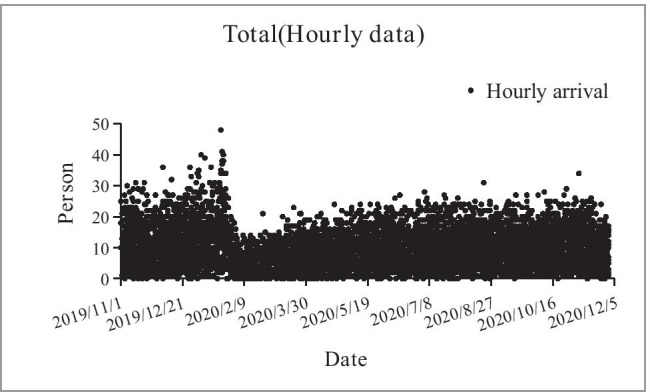
Scatter plot of ED patient arrival hourly data (November 1, 2019 - November 30, 2020)

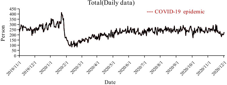
We can see from Fig. 1 that the number of patient arrivals gradually increases over time, then declines stepwise, and eventually flattens out gradually. The highest point was reached from 7:00 pm to 8:00 pm on January 21, 2020, with 48 records, and an average of 1.25 patients arrived every minute. Figure 2 shows the daily change in the number of patient arrivals. The red dotted region indicates the period of COVID-19 epidemic changes in emergency patient arrivals. When the COVID-19 epidemic had just started, people did not undertake protective measures, which led to a surge in emergency patients [25]. Through government and medical unit control, noncritical patients were prohibited from going to hospitals, and the number of emergency patients fell to the lowest point. With the COVID-19 epidemic under control, the number of ED patients gradually returned to normal.

Fig. 2.

Daily patient arrival flows (November 1, 2019 - November 30, 2020)

In the original meteorological data, there were many missing values in certain fields that made the training model meaningless, so these fields were deleted to avoid affecting the results. For a field with a small number of missing values, observe whether it is continuous or discrete. For missing continuous data, fill it with the average value of the week. If it is discrete, use the value of the previous day.

Considering that drastic changes in climate and environmental factors may have an impact on human health, the difference between the day and the previous day for some features was calculated as a new feature and added to the original data. Table 1 defines the details for the initial feature collection. For hourly data, X3, X11 to X18, and X19 to X29 were not included. For hourly patient arrival data, the month and air quality data have no mean for model forecasting; for daily data, X1 and X3 were not included, and other features were combined for selection and then input into the model. In addition, some calendar and meteorological data were converted into numerical variables to obtain better forecasting results.

Table 1.

Original feature data details

Feature type	Feature No.	Description	Value meaning
Calendar data	X1	Hour of day	Continuous variable
	X2	Day of week	Continuous variable
	X3	Month of year	Continuous variable
	X4	Season of year	0 = Spring, 1 = Summer, 2 = Autumn, 3 = Winter
	X5	Public holiday	0 = No Public Holiday, 1 = Public holiday
Meteorological data	X6	Air temperature(max)	Continuous variable (deg. C)
	X7	Air temperature(mean)	Continuous variable (deg. C)
	X8	Air temperature(min)	Continuous variable (deg. C)
	X9	Mean wind speed level	Continuous variable
	X10	Weather	0 = Sunny, 1 = Cloudy, 2 = Overcast, 3 = Light rain, 4 = Heavy rain, 5 = Snow
	X11-X18	Air quality index related data	Continuous variable
Newly constructed data	X19-X29	Change of X6 to X9, X11, X13 to X18 compared with one day before	Continuous variable

Since each data point comes from different sources and has different dimensions, to eliminate the impact of the range and reduce the model error, the data were normalized between 0 and 1. The normalization process is shown in (1) as follows.

$$X_{\mathit{nor}}=\frac{X-X_{\mathit{min}}}{X_{\mathit{max}}-X_{\mathit{min}}}$$ 1

where $X$ represents the value of each feature, $X_{\mathit{max}}$ represents the maximum value of each feature, $X_{\mathit{min}}$ represents the minimum value of each feature, and $X_{\mathit{nor}}$ represents the final normalized value.

Kernel Principal Component Analysis

Kernel principal component analysis (KPCA) is based on the principle of the kernel function. It projects the input space to the high-latitude feature space through nonlinear mapping, and then performs principal component analysis on the mapped data in the high-latitude space, which has strong nonlinear processing capabilities. The kernel method can transform nonlinear data into linear data by increasing the dimension, thereby solving part of the nonlinear problem. The commonly used kernel functions have the following forms:

Linear kernel:

$$K\left(x,,,x_i\right)=<x,x_i>$$ 2

Poly kernel:

$${K\left(x,,,x_i\right)=(<x,x_i>+1)}^p$$ 3

RBF kernel:

$${K\left(x,,,x_i\right)=exp\left(\frac{-\Vert x-x_i{\Vert }^2}{{\sigma }^2}\right)}^p$$ 4

Maximal Information Coefficient

For daily data, since the arrival of patients is affected by many factors, it is impossible to use linear correlation methods to analyze the complicated nonlinear relationship between the features. The concept of the maximal information coefficient (MIC) was first proposed by Reshef et al. in Science in 2011. Compared with other correlation calculation algorithms, the MIC method can not only calculate the linear correlation between parameters but also calculate the nonlinear correlation, which has better search performance. The calculation equations of the maximum information coefficient can be expressed as:

$$I(D,x,y)=\sum _{xeX,yeY}p(x,y)log\left(\frac{p(x,y)}{p\left(x\right)p\left(y\right)}\right)$$ 5

$$M\left(D\right)x,y=\frac{I(D,x,y)}{log\left(m,i,n,\left\{x,,,y\right\}\right)}$$ 6

Equation (5) is the formula for solving the maximum correlation coefficient. The maximum correlation between variables is found through a grid search; the denominator in Eq. (6) is used to avoid differences in different dimensions after normalization of the impact.

Machine learning algorithms

The widely used machine learning algorithms selected in this paper are linear regression, KNN, SVR, ridge, XGBoost, random forest, AdaBoost, gradient boosting, bagging and LSTM, most of which have good performance in multiple fields. Some brief introductions of the above algorithms are shown in Table 2.

Table 2.

Advantages and disadvantages of using algorithms

Algorithm	Advantage	Disadvantage
Linear Regression	Simple thinking, easy to implement, especially effective for small data volumes	It is difficult to model polynomial regressions for nonlinear data
KNN	The algorithm is simple, and the training time complexity is O(n)	Large amounts of calculation when there are more features
SVR	Suitable for small sample data, can solve high-dimensional problems	Sensitive to missing values and high memory consumption
Ridge	The penalty will reduce overfitting	No feature selection function
Xgboost	1. Distributed processing of high-dimensional features 2. The importance of features can be output 3. Add regular term to reduce fitting	Iterative data consumes more space
Random Forest	Can handle high-dimensional data without feature selection	Different attribute division methods have a greater impact on the forecast effect
AdaBoost	High accuracy without overfitting	Training time is too long, and easy to be disturbed by noise
Gradient Boosting	The forecast effect is stable and robust	High computational complexity and not easy to parallelize
Bagging	Integrated multiple regressors, with better prediction results	Larger digestion space
LSTM	Suitable for dealing with problems that are highly related to time series	The amount of calculation will be huge and time-consuming

Evaluation indicators

The stability and results of the model are evaluated by three indicators.

• (1) Root mean squared error

  $$RMSE=\sqrt{\frac{1}{n}\sum _{i=1}^n{\left(\widehat{y_i},-,y_i\right)}^2}$$ 7

where $\widehat{y_i}$ is the forecast value, $y_i$ is the true value, and $n$ is the sample number. The greater the error, the greater the value.

• (2) Mean absolute error

  $$MAE=\frac{1}{n}\sum _{i=1}^n\left|\widehat{y_i},-,y_i\right|$$ 8

where $\widehat{y_i}$ is the forecast value, $y_i$ is the true value, and $n$ is the sample number. The greater the error, the greater the value.

• (3) Mean absolute percentage error

  $$MAPE=\frac{100\%}{n}\sum _{i=1}^n\left|\frac{\widehat{y_i}-y_i}{y_i}\right|$$ 9

where $\widehat{y_i}$ is the forecast value, $y_i$ is the true value, and $n$ is the sample number. When the true value has data equal to 0, the formula is not available.

Results and discussion

We observed 90,783 ED patient arrival data points during the period from November 1, 2019, to November 30, 2020, 396 day records. We divided the records from November 1, 2019, to August 31, 2020, as the training set and September 1, 2020, to November 31, 2020, as the test set. Boxplots of the patient arrival distribution by hour of the day, day of the week, and season of the year are shown in Fig. 3.

Fig. 3.

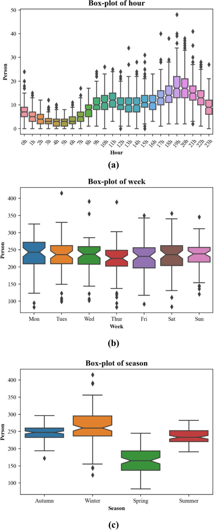
Box-plots of ED patient arrivals by (a) hour of the day, (b) day of the week, and (c) season of the year

It can be seen from Fig. 3 that due to various factors, there is a small volume of noise in the original sample. These noise points can cause underfitting of the forecast model and impact the forecast effect if the noise is not processed. Therefore, in this paper, noise larger than the upper bound of the sample is smoothed to the upper bound of the sample; noise smaller than the lower bound of the sample is smoothed to the sample’s lower bound.

Forecast result for the hourly data

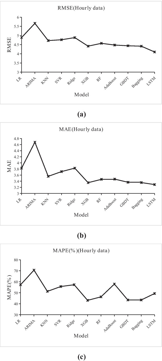
For hourly data forecasting, features X3, X11 to X29 in Table 1 are not included. The model parameter settings are shown in Table 3, and Fig. 4 shows the results of the hourly data forecast models.

Table 3.

Parameter settings of the data forecast

Model	Parameter settings
Linear regression	Default
KNN	N_neighbors = 3
SVR	Kernel = RBF, C = 1e3, epsilon = 0.1
Ridge	Alpha = 1.0, normalize = False
Xgboost	Eta = 0.1, max_depth = 9, gamma = 0.1
Random forest	N_jobs = 1, random_state = 12, n_estimators = 100
AdaBoost	Default
Gradient boosting	Max_depth = 9, min_sample_split = 200
Bagging	Base_estimator = ‘decision tree’
LSTM	Step_size = 4, epochs = 300

Fig. 4.

The results of ten hourly forecast models and ARIMA evaluated by (a) RMSE, (b) MAE, and (c) MAPE

It can be seen from the boxplot of hours of the day in Fig. 3 that the number of ED patient arrivals was more concentrated in 19:00 pm and 20:00 pm and Mondays presented the highest ED patient arrivals while Thursday presented the lowest. In addition, the season was also the main factor affecting the arrival of patients. Winter is a period of high incidence of cardiovascular and cerebrovascular diseases, which increases the volumes of patient. We calculated the RMSE, MAE, and MAPE of each model and compared their accuracy to show which model would be the most useful in hourly data forecasting in Fig. 4. Compared with the traditional ARIMA model, it can be seen that regardless of RMSE, MAE and MAPE, the ten models perform better than ARIMA. In addition, with the addition of calendar variables and weather information, Xgboost, random forest, AdaBoost, gradient boosting, and bagging are all ensemble learning methods that have better performance in terms of RMSE and MAE. Ensemble learning is based on an ensemble of multiple learning algorithms to improve the forecast results. Additionally, LSTM is Suitable for dealing with problems that are highly related to time series, which perform best in RMSE and MAE, but it is higher than the ensemble model in Mape. Through the above model comparison, hourly patient arrival forecasting is suitable for the use of LSTM and ensemble learning models.

Forecast result for the daily data

For daily data forecasting, all the features may affect patient arrivals. Moreover, similar input features may also introduce different effects into the forecast results [2]. Therefore, this paper uses two feature selection methods to compare the forecast results: one is the daily forecast result with KPCA, and the other is the daily forecast result with MIC-KPCA. The model parameter settings are the same as those shown in Table 3.

Daily forecast result with KPCA

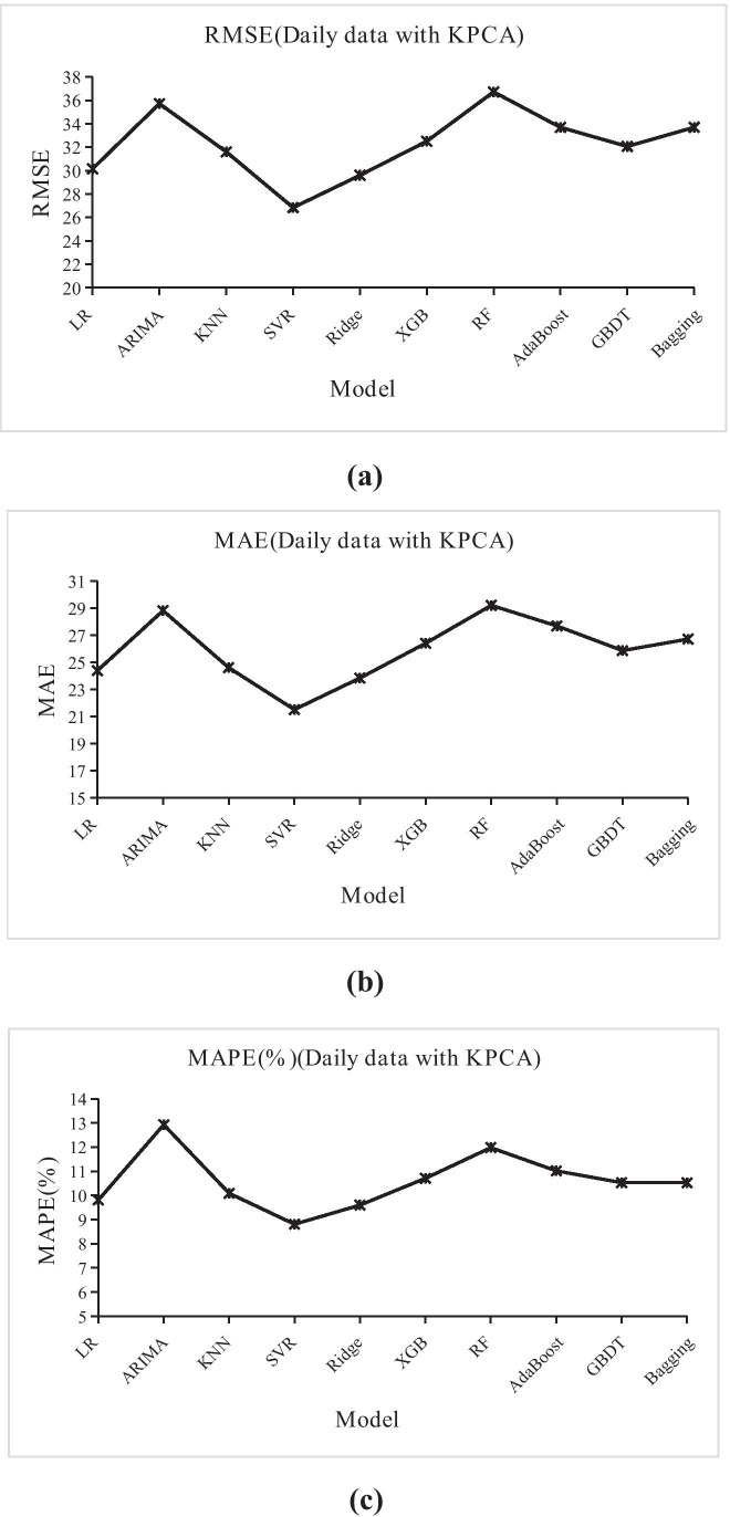
We used KPCA for nonlinear dimensionality reduction with all of the features except X1 and X3 in Table 1, where the parameter settings of KPCA were kernel: RBF, gamma: 10, n_components: 5, and the other parameters were the default. Figure 5 shows the results of the daily forecast with KPCA.

Fig. 5.

The results of nine daily forecasts with the KPCA models and the ARIMA model evaluated by (a) RMSE, (b) MAE, and (c) MAPE

Daily forecast result with MIC-KPCA

In Section 3.2.1, we perform KPCA dimensionality reduction processing on all features for daily forecasting, but some irrelevant features may affect the dimensionality reduction result. Therefore, we use the MIC method to select features that are relevant to patient arrivals first, and then reduce the dimensions of these features to forecast the result. The correlation between the features and patient arrivals is shown in Table 4. Finally, we chose X4, X8-X9, X11-X14, X16-X20, X23-X24 and X27-X28 as the input of KPCA, in which the MIC coefficients between daily patient arrivals are both above 0.1.

Table 4.

MIC coefficients between each feature and the daily patient arrivals

Feature No.	MIC coefficients	Feature No.	MIC coefficients
X2 X4 X5 X6 X7 X8 X9 X10 X11 X12 X13 X14 X15 X16	0.02 0.7 0.03 0.05 0.08 0.11 0.17 0.09 0.35 0.3 0.28 0.2 0.06 0.36	X17 X18 X19 X20 X21 X22 X23 X24 X25 X26 X27 X28 X29	0.35 0.16 0.13 0.11 0.01 0.03 0.18 0.18 0.05 0.01 0.23 0.16 0.04

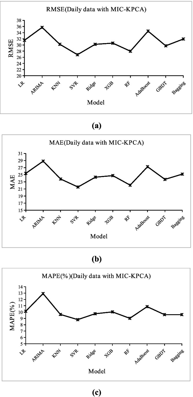
The parameter settings of KPCA are the same as those in Section 3.2.1. Figure 6 shows the results of the daily forecast with MIC-KPCA.

Fig. 6.

The results of nine daily forecasts with the MIC-KPCA models and the ARIMA model evaluated by (a) RMSE, (b) MAE, and (c) MAPE

We can see from Fig. 5 in Section 3.2.1 that when the KPCA method is used directly on the original feature data to eliminate redundant information between features, the machine learning models we used performed better than the ARIMA model, except for random forests. This may be due to the limited volume of data, but its MAPE value is lower than that of ARIMA. Considering that irrelevant factors will have an impact on the results, we use the MIC approach to screen out feature specific patient arrivals and reduce dimensionality. The results can be seen in Fig. 6, Except for LR, the RMSE, MAE, and MAPE of all machine learning models with MIC-KPCA are lower than those with KPCA, which shows that similar factors do affect the results, while the MIC method can select the most relevant features to make better predictions. However, although the LSTM model perform best in hourly data forecast, whether it is daily forecast result with KPCA or daily forecast result with MIC-KPCA, LSTM is under-fitting, which make the forecast results have a large error with the actual data. Maybe because of the small amount of daily data. The daily forecast results of the two feature selection methods are shown in Table 5 (except LSTM model).

Table 5.

Daily forecast results of the two feature selection methods

Model	Daily forecast result with KPCA			Daily forecast result with MIC-KPCA
	RMSE	MAE	MAPE(%)	RMSE	MAE	MAPE(%)
Linear Regression	30.16	24.4	9.81	31.52	25.39	10.13
ARIMA	35.72	28.83	12.93	35.72	28.83	12.93
KNN	31.61	24.62	10.09	30.23	23.79	9.63
SVR	26.84	21.52	8.81	26.84	21.53	8.81
Ridge	29.6	23.85	9.6	30.21	24.31	9.74
Xgboost	32.51	26.42	10.71	30.6	24.75	10.03
Random Forest	36.73	29.22	11.98	27.98	22.06	9.02
AdaBoost	33.7	27.7	11.02	34.5	27.26	10.86
Gradient Boosting	32.07	25.88	10.53	29.73	23.69	9.6
Bagging	33.7	26.73	10.53	31.94	25.17	9.6

From the daily forecast results of the two feature selection methods, We found that calendar variables were more important forecasting factors than temperature data. By using the MIC method to reduce the impact of other irrelevant variables, our results found that compared with the daily forecast result with KPCA, the RMSE, MAE, and MAPE of the Xgboost, random forest, Adaboost, gradient boosting, and bagging models have all decreased significantly. Therefore, the selection of forecast variables still remains challenging.

However, what is surprising is that regardless of the feature selection method, the performance of ensemble learning is not as good as SVR. The MAPE of SVR is the lowest among all of the models, at 8.8%. [26] found that a less complex moving average model had the best forecasting result. Even though complex forecasting models in general give a better fit than simpler models, the resulting forecast is not necessarily more accurate, and simpler models are often better. Additionally, the advantage of SVR shown in Table 1 that it is suitable for small sample data and can solve high-dimensional problems. Therefore, SVR has the best effect on daily patient arrival forecasts based on two feature selection methods.

Conclusions

Starting from reality, this paper considers the particularity of the ED and uses ten machine learning methods to construct an emergency patient arrival forecast model based on calendar and meteorological information. For hourly patient arrival forecasting, each machine learning model has better forecast results than the traditional ARIMA model, especially the LSTM and ensemble learning models, such as XGBoost, random forest, gradient boosting, and bagging. For daily patient arrival forecasting, this paper proposed two feature selection methods to compare the results. The results show that the feature selection method based on MIC-KPCA has a better overall forecast effect. In addition, it is found that LSTM performed better in the hourly data forecast and in the daily patient arrivals forecast the simpler models are often better than the ensemble models. Based on this, the following conclusions are proposed:

1. Calendar and meteorological information have a significant influence on ED patient arrival forecasts.

2. The feature selection method based on MIC-KPCA performs better in daily patient arrival forecasting and can serve as the management baseline to better allocate ED personnel and medical resources.

3. For hourly patient arrival forecasts, LSTM model has best forecast result than ensemble learning models in RMSE and MAE, while for daily patient arrival forecasts, simpler models often perform better.

This paper only forecast the ED patient arrivals. However, different patients have different severities. How to perform cluster analysis to forecast patients under different severities will be the focus of the author’s future research.

Yan Zhang

received his Master’s degree from Nanchang Hangkong University. His main research interest is wireless sensor networks and data mining.

Author contributions

Yan Zhang analyzed the data and drafted the manuscript. Jie Zhang designed the research. Min Tao, Jian Shu, Degang Zhu conducted the research. All authors read and approved the fnal manuscript.

Funding

This work was funded by Anhui Province Health Soft Science Research Project (Approval No: 2020WR02016).

Data availability

The datasets generated and/or analyzed during the current study are not publicly available due to ethical and legal reasons but are available from the corresponding author on reasonable request.

Declarations

Consent for publication

Not applicable.

Competing interest

The authors declare that they have no competing interests.

Conflict of interest

The authors declare that there are no conflicts of interest in this work.

References

- 1.Sinha A, Rathi M (2021) COVID-19 prediction using AI analytics for South Korea. Appl Intell. 10.1007/s10489-021-02352-z [DOI] [PMC free article] [PubMed]
- 2.Jiang S, Chin K-S, Tsui KL. A universal deep learning approach for modeling the flow of patients under different severities. Comput Methods Programs Biomed. 2018;154:191–203. doi: 10.1016/j.cmpb.2017.11.003. [DOI] [PubMed] [Google Scholar]
- 3.Xu M, Wong TC, Chin KS. Modeling daily patient arrivals at Emergency Department and quantifying the relative importance of contributing variables using artificial neural network. Decis Support Syst. 2013;54(3):1488–1498. doi: 10.1016/j.dss.2012.12.019. [DOI] [Google Scholar]
- 4.Afilal M, Yalaoui F, Dugardin F, Amodeo L, Laplanche D, Blua P. Forecasting the emergency department patients flow. J Med Syst. 2016;40(7):175. doi: 10.1007/s10916-016-0527-0. [DOI] [PubMed] [Google Scholar]
- 5.Jilani T, Housley G, Figueredo G, Tang P-S, Hatton J, Shaw D. Short and Long term predictions of Hospital emergency department attendances. Int J Med Inform. 2019;129:167–174. doi: 10.1016/j.ijmedinf.2019.05.011. [DOI] [PubMed] [Google Scholar]
- 6.Harrou F, Dairi A, Kadri F, Sun Y. Forecasting emergency department overcrowding: A deep learning framework. Chaos Solitons Fract. 2020;139:110247. doi: 10.1016/j.chaos.2020.110247. [DOI] [PMC free article] [PubMed] [Google Scholar]
- 7.Pak A, Gannon B, Staib A. Predicting waiting time to treatment for emergency department patients. Int J Med Inform. 2021;145:104303. doi: 10.1016/j.ijmedinf.2020.104303. [DOI] [PubMed] [Google Scholar]
- 8.Carvalho-Silva M, Monteiro MTT, Sá-Soares FD, Dória-Nóbrega S. Assessment of forecasting models for patients arrival at Emergency Department. Oper Res Health Care. 2018;18:112–118. doi: 10.1016/j.orhc.2017.05.001. [DOI] [Google Scholar]
- 9.Barak S, Sadegh SS. Forecasting energy consumption using ensemble ARIMA–ANFIS hybrid algorithm. Int J Electr Power Energy Syst. 2016;82:92–104. doi: 10.1016/j.ijepes.2016.03.012. [DOI] [Google Scholar]
- 10.Aboagye-Sarfo P, Mai Q, Sanfilippo FM, Preen DB, Stewart LM, Fatovich DM. A comparison of multivariate and univariate time series approaches to modelling and forecasting emergency department demand in Western Australia. J Biomed Inform. 2015;57:62–73. doi: 10.1016/j.jbi.2015.06.022. [DOI] [PubMed] [Google Scholar]
- 11.Rosychuk RJ, Youngson E, Rowe BH. Presentations to Alberta emergency departments for asthma: a time series analysis. Acad Emerg Med. 2015;22(8):942–949. doi: 10.1111/acem.12725. [DOI] [PubMed] [Google Scholar]
- 12.Cheng Q, Argon NT, Evans CS, Liu Y, Platts-Mills TF, Ziya S. Forecasting emergency department hourly occupancy using time series analysis. Am J Emerg Med. 2021;48:177–182. doi: 10.1016/j.ajem.2021.04.075. [DOI] [PubMed] [Google Scholar]
- 13.Becerra M, Jerez A, Aballay B, Garcés HO, Fuentes A. Forecasting emergency admissions due to respiratory diseases in high variability scenarios using time series: A case study in Chile. Sci Total Environ. 2020;706:134978. doi: 10.1016/j.scitotenv.2019.134978. [DOI] [PubMed] [Google Scholar]
- 14.Khaldi R, Afia AE, Chiheb R. Forecasting of weekly patient visits to emergency department: real case study. Procedia Comput Sci. 2019;148:532–541. doi: 10.1016/j.procs.2019.01.026. [DOI] [Google Scholar]
- 15.Li J, Li BY, Wei ZJ, Zhao YZ, Li TS (2020) Application research on gated recurrent unit deep learning prediction and graded early warning of emergency department visits based on meteorological environmental data. Biomed Environ Sci 33(10):817–820. 10.3967/bes2020.111 [DOI] [PubMed]
- 16.Schluck G, Wu W, Whyte J, Abbott L. Emergency department arrival times in Florida heart failure patients utilizing Fisher-Rao curve registration: A descriptive population-based study. Heart Lung. 2018;47(5):458–464. doi: 10.1016/j.hrtlng.2018.05.020. [DOI] [PubMed] [Google Scholar]
- 17.Saleh R, Makki M, Tamim H, Hitti E. The impact of ramadan on patient attendance patterns in an Emergency Department at a Tertiary Care Center in Beirut, Lebanon. J Emerg Med. 2020;59(5):720–725. doi: 10.1016/j.jemermed.2020.06.039. [DOI] [PubMed] [Google Scholar]
- 18.Kuo Y-H, Chan NB, Leung JMY, Meng H, So AM-C, Tsoi K K F, Graham CA. An integrated approach of machine learning and systems thinking for waiting time prediction in an emergency department. Int J Med Inform. 2020;139:104143. doi: 10.1016/j.ijmedinf.2020.104143. [DOI] [PubMed] [Google Scholar]
- 19.Menke NB, Caputo N, Fraser R, Haber J, Shields C, Menke MN. A retrospective analysis of the utility of an artificial neural network to predict ED volume. Am J Emerg Med. 2014;32(6):614–617. doi: 10.1016/j.ajem.2014.03.011. [DOI] [PubMed] [Google Scholar]
- 20.Sudarshan VK, Brabrand M, Range TM, Wiil UK. Performance evaluation of Emergency Department patient arrivals forecasting models by including meteorological and calendar information: A comparative study. Comput Biol Med. 2021;135:104541. doi: 10.1016/j.compbiomed.2021.104541. [DOI] [PubMed] [Google Scholar]
- 21.Liu Y, Yang C, Huang K, Gui W. Non-ferrous metals price forecasting based on variational mode decomposition and LSTM network. Knowl Based Syst. 2020;188:105006. doi: 10.1016/j.knosys.2019.105006. [DOI] [Google Scholar]
- 22.Chen S-M, Zou X-Y, Gunawan GC. Fuzzy time series forecasting based on proportions of intervals and particle swarm optimization techniques. Inf Sci. 2019;500:127–139. doi: 10.1016/j.ins.2019.05.047. [DOI] [Google Scholar]
- 23.Zhang R, Zhang Z, Wang D, Du M. Feature selection with multi-objective genetic algorithm based on a hybrid filter and the symmetrical complementary coefficient. Appl Intell. 2021;51(6):3899–3916. doi: 10.1007/s10489-020-02028-0. [DOI] [Google Scholar]
- 24.Sun G, Li J, Dai J, Song Z, Lang F. Feature selection for IoT based on maximal information coefficient. Futur Gener Comput Syst. 2018;89:606–616. doi: 10.1016/j.future.2018.05.060. [DOI] [Google Scholar]
- 25.Caro JJ, Möller J, Santhirapala V, Gill H, Johnston J, El-Boghdadly K, Santhirapala R, Kelly P, Mcguire A. Predicting hospital resource use during COVID-19 surges: a simple but flexible discretely integrated condition event simulation of individual patient-hospital trajectories. Value Health. 2021 doi: 10.1016/j.jval.2021.05.023. [DOI] [PMC free article] [PubMed] [Google Scholar]
- 26.Marcilio I, Hajat S, Gouveia N. Forecasting daily emergency department visits using calendar variables and ambient temperature readings. Acad Emerg Med. 2013;20(8):769–777. doi: 10.1111/acem.12182. [DOI] [PubMed] [Google Scholar]
Associated Data
This section collects any data citations, data availability statements, or supplementary materials included in this article.
Data Availability Statement