Q2DW-Tide and -Ionosphere Interactions as Observed From ICON and Ground-Based Radars

Abstract

A quasi-2-day wave (Q2DW) event during January-February, 2020, is investigated in terms of its propagation from 96 to 250 km as a function of latitude (10°S to 30°N), its nonlinear interactions with migrating tides to produce 16 and 9.6-h secondary waves (SWs), and the plasma drift and density perturbations that it produces in the topside F-region (590–607 km) between magnetic latitudes 18°S and 18°N. This is accomplished through analysis of coincident Ionospheric Connections Explorer (ICON) measurements of neutral winds, plasma drifts and ion densities, and wind measurements from four low-latitude (±15°) specular meteor radars (SMRs). The Q2DW westward-propagating components that existed during this period consist of zonal wavenumbers s = 2 and s = 3, that is, Q2DW+2 and Q2DW+3 (e.g., He, Chau et al., 2021, https://doi.org/10.1029/93jd00380). SWs in the ICON measurements are inferred from Q2DW+2 and Q2DW+3 characteristics derived from traditional longitude-UT fits that potentially contain aliasing contributions from SWs (“apparent” Q2DWs), from fits to space-based zonal wavenumbers that each reflect the aggregate signature of either Q2DW+2 or Q2DW+3 and its SWs combined (“effective” Q2DWs), and based on information contained in published numerical simulations. The total Q2DW ionospheric responses consists of F-region field-aligned and meridional drifts of order ±25 ms⁻¹ and ±5–7 ms⁻¹, respectively, and total ion density perturbations of order (±10%–25%). It is shown that the SWs can sometimes make substantial contributions to the Q2DW winds, drifts, and plasma densities.

1. Introduction

Quasi-2-day oscillations (Q2DOs) represent a prominent component of mesospheric dynamics in Earth’s atmosphere, and exist in three forms (Pancheva et al., 2016): Eastward-propagating Q2DOs exist at middle to high-latitudes during winter, and are thought to be generated by jet instabilities. They also occur more sporadically in the equatorial region in the form of ultra-fast Kelvin waves (UFKW). The Q2DO that is the subject of the present paper is the global-scale westward-propagating quasi-two-day wave (hereafter, Q2DW) that originates during summer seasons in both hemispheres, albeit with somewhat different dominant periods and zonal structures. The Q2DW has been extensively studied from the ground (e.g., Craig et al., 1980; Doyle, 1968; Fritts & Isler, 1994; Fritts et al., 1999; Gurubaran et al., 2001; Lima et al., 2004; Malinga & Ruohoniemi, 2007; Meek et al., 1996; Müller, 1972; Müller & Kingsley, 1974; Müller & Nelson, 1978; Palo & Avery, 1995; Pancheva et al., 2004; Pancheva, 2006; Raghava Reddi et al., 1988; Salby & Roper, 1980; Thayaparan et al., 1997; Zhou et al., 1997) and space (Chang et al., 2014; Ern et al., 2013; Fritts et al., 1999; Garcia et al., 2005; Gu et al., 2013; Huang et al., 2013; Lieberman, 1999; Limpasuvan et al., 2005; Limpasuvan & Wu, 2009; Moudden & Forbes, 2014; Pancheva et al., 2018; Rodgers & Prata, 1981; Tunbridge et al., 2011; Ward et al., 1996; Wu et al., 1993) mainly below 100 km, although a few of the cited references reported Q2DW observations up to 140 km (Ward et al., 1996; Wu et al., 1993; Zhou et al., 1997). The Q2DW has also been studied in the context of two-dimensional (latitude-height) steady-state models (Hagan et al., 1993; Nguyen et al., 2016; Salby, 1981) and general circulation models (GCMs, e.g., Chang et al., 2011; Gu, Liu, Li, Dou, et al., 2015; Gu et al., 2016, 2018; Lieberman et al., 2017; McCormack et al., 2009, 2010; Norton & Thuburn, 1996; Palo et al., 1999; Pancheva et al., 2016; Wang et al., 2017; Yue, Liu, & Chang, 2012).

Over 3 decades ago it was recognized that the Q2DW plays a significant role in atmosphere-ionosphere (A-I) coupling, and thus in day-to-day variability of the ionosphere (e.g., Chen, 1992; Ito et al., 1986; Pancheva, 1988; Pancheva & Lysenko, 1988). It was not until the most recent decade that GCMs including ionospheric electrodynamics have become available to provide new insights into A-I coupling by the Q2DW (e.g., Gu, Liu, Li, & Dou, 2015; Gu et al., 2018; Yue, Liu, & Chang, 2012; Yue, Wang et al., 2016). In particular, these works point to the role of secondary waves (SWs) due to Q2DW-tide nonlinear interactions in adding complexity to the spatial-temporal response of the ionosphere to the Q2DW. However, a remaining impediment to our understanding of Q2DW A-I coupling is the paucity of wind measurements, particularly at low latitudes, and in the ionospheric E-region (100–150 km) where the dynamo generation of electric fields occurs. Q2DW wind measurements near the equator during austral summer are relatively few (i.e., Gurubaran et al., 2001; Harris & Vincent, 1993; Palo & Avery, 1995; Pancheva, 2006; Raghava Reddi et al., 1988; Ward et al., 1996; Wu et al., 1993), but achieve amplitudes of order 20–40 ms⁻¹ around 90–100 km, and can maintain similar amplitudes between 20°–40° latitude in the Northern Hemisphere (NH) (Fritts & Isler, 1994; Fritts et al., 1999; Ward et al., 1996). However, given the sensitivity of Q2DW vertical propagation to the zonal-mean zonal wind distribution (Yue, Liu, & Chang, 2012), vertical penetration into the dynamo region can never be assured based on observations at lower altitudes. Moreover, the existence of SWs due to Q2DW-tide interactions in low-latitude observations has barely been mentioned, except for Harris and Vincent (1993), Moudden and Forbes (2014) and Pancheva (2006). It should be evident from the above brief review that there have been no observational studies to date that measure winds in the E- and F-regions concurrently with the F-region ionospheric response.

The Q2DW is traditionally studied in terms of its zonal harmonic components. This initially arose from the Q2DW being identified as an atmospheric normal mode; that is, a westward-propagating mixed Rossby-gravity wave with zonal wavenumber s = 3 (Salby, 1981), hereafter Q2DW+3. However, soon afterward theory developed to admit the possibility that the Q2DW could be forced by baroclinic instability of the summer middle atmosphere easterly jet (Plumb, 1983; Pfister, 1985), which admits zonal wavenumbers of m = 2 − 4; furthermore, the Q2DW+3 normal mode can also be amplified by this instability (Randel, 1994; Salby & Callaghan, 2000). In principle the Q2DWs with s = 2 and s = 4 (hereafter Q2DW+2 and Q2DW+4) can also be generated through nonlinear interaction between Q2DW+3 and the stationary planetary wave with s = 1 (SPW1) (Gu, Liu, Li, & Dou, 2015). The potentially variable longitude structure of the Q2DW means that Q2DW measurements at a given latitude, height or time from a single ground-based (G-B) site cannot provide information on which zonal harmonic(s) might be present. Several studies employing G-B measurements of the Q2DW have derived, or placed bounds on, the zonal wavenumbers of the Q2DW (Meek et al., 1996; Malinga & Ruohoniemi, 2007; Pancheva et al., 2004; He, Forbes, et al., 2021; He, Chau et al., 2021; Meek et al., 1996; Malinga & Ruohoniemi, 2007; Pancheva et al., 2004) however, these studies are relatively limited and infrequent. On the other hand, the satellite-based measurements enumerated above generally delineate longitudinal structures and zonal wavenumbers, but suffer from crude temporal resolution and aliasing, which is discussed in more detail in Section 2. The net result is that it is not possible to observationally specify the dynamo-region wind field from satellite-based measurements in a way that is free from ambiguities.

In He, Forbes, et al. (2021), dual-station G-B data were used to determine the periods and zonal wavenumbers of Q2DW+3 and Q2DW+4 winds and their temporal evolutions, as well as of secondary waves due to Q2DW-tide interactions. That study was performed at middle latitudes during Northern Hemisphere (NH) summer. He, Chau et al. (2021) (hereafter Paper #1) subsequently applied the same techniques to four low-latitude (±20° latitude) radars to similarly study Q2DW+2 and Q2DW+3 winds during January–March, 2020. They obtained mostly excellent agreement with Q2DW wind measurements made by the MIGHTI (Michelson Interferometer for Global High-resolution Thermospheric Imaging) on NASA’s ICON (Ionospheric CONnection explorer) satellite (Immel et al., 2018) in the overlapping height region of 95–100 km. ICON/MIGHTI observations were also employed to provide the first measurements of Q2DW+2 and Q2DW+3 winds over the 100–200 km height range from 9°S–30°N latitude during austral summer. It is the purpose of the present work to extend the data analysis of Paper #1 to examine, for the first time, the ionospheric response to the Q2DW using concurrent measurements of thermospheric winds, F-region drifts and F-region plasma densities. We also take this opportunity to obtain insight into the presence and potential role of secondary waves in the Q2DW A-I coupling process through the use of both G-B and satellite-based (S-B) data.

In the following the tidal and planetary wave nomenclature used in this paper is briefly reviewed. The following section includes a discussion of SWs in S-B measurements of the Q2DW, the aliasing that accompanies the presence of SWs, and a perspective that seeks to bring some clarity to the experimental determination of Q2DWs from space.

2. Special Considerations for the Q2DW When Viewed From Space

2.1. Tidal and Planetary Wave Nomenclature

The expression

$$A_{n,s}\cos \left(n\text{Ω}t+s\lambda -{\varphi }_{n,s}\right)$$ (1)

represents a tidal oscillation in any atmospheric variable (e.g., temperature, wind speed, etc.), where A_n,s is its amplitude; n = 1, 2, 3 refers to diurnal, semidiurnal and terdiurnal periods, respectively; Ω = 2π d⁻¹; s is the zonal wavenumber; λ is longitude; and ϕ_n,s is its phase (time of amplitude maximum at λ = 0, or longitude of maximum at t = 0). Setting the quantity in parentheses equal to a constant and differentiating yields the zonal phase speed of the tide, C_ph = − nΩ/s. A Sun-synchronous tide that follows the westward motion of the Sun to a G-B observer (−Ω), i.e., s = n, is traditionally referred to as a migrating tide; otherwise it is said to be non-migrating (Chapman & Lindzen, 1970). By convention, DWs or DEs denote a westward or eastward-propagating diurnal tide, respectively, with zonal wavenumber = s. For semidiurnal and terdiurnal oscillations “S” and “T” respectively replace “D”. D0, S0, T0 denote the zonally-symmetric oscillations. Similarly, planetary waves (PWs) are expressed as

$$A_{\delta ,m}\cos \left(\delta \text{Ω}t+m\lambda -{\varphi }_{\delta ,m}\right)$$ (2)

where δ < 1.0 and m is an integer zonal wavenumber. If δ ≠ 0 the waves are said to be traveling in the zonal direction, eastward if m < 0 and westward if m > 0 for the adopted sign convention. If δ = 0 the waves are said to be stationary planetary waves (SPW) with zonal wavenumber m, and are designated SPWm.

2.2. SWs Due to Q2DW-Tide Interactions and Aliasing

The SWs that arise from wave-wave interactions can be expressed based on the quasi-linear theory put forth by Teitelbaum and Vial (1991), which states that when two primary waves with (frequency, zonal wavenumber) = (σ₁, s₁) and (σ₂, s₂) interact, that secondary waves are produced with the sum and difference frequencies and zonal wavenumbers of the primary waves, that is, (σ₁ + σ₂, s₁ + s₂) and (σ₁ − σ₂, s₁ − s₂). The generation of SWs along these lines is now rather well accepted due to its widespread verification in analyses of observations (e.g., Beard et al., 1999; Cevolani & Kingsley, 1992; Forbes & Moudden, 2012; Forbes & Zhang, 2017; Gasperini et al., 2015; Huang, Liu, Zhang et al., 2013; Huang, Liu, Lu et al., 2013; Kamalabadi et al., 1997; Pancheva et al., 2000, 2002; Pancheva & Mitchell, 2004; Rüster, 1994; Xu et al., 2014) and GCMs (e.g., Gan et al., 2017; Nystrom et al., 2018; Palo et al., 1999; Pedatella & Forbes, 2012). The problem of aliasing in connection with satellite-based (S-B) measurements of the Q2DW and its interactions with tides is also well-known and documented in the literature (e.g., Forbes & Moudden, 2012; Nguyen et al., 2016; Tunbridge et al., 2011), and basically exists because tidal frequencies (e.g., 1.0, 2.0, 3.0 d⁻¹, …) are near-integer multiples of the Q2DW frequency ≈ 0.5 d⁻¹. Converting (Equation 1) from universal time to local solar time (LST), that is, t = t_LST − λ/Ω:

$$A_{\delta ,m}\cos \left(\delta \text{Ω}{t}_{LST}+\left(m-\delta \right)\lambda -{\varphi }_{\delta ,m}\right),$$ (3)

we see that when viewed from a quasi-Sun-synchronous (t_LST ≈ constant) S-B perspective, a Q2DW appears as a longitudinal structure defined by its “S-B zonal wavenumber” k_s = |m − 0.5|. For example, a Q2DW with m = −2 (Q2DW-2) and a Q2DW with m = +3 (Q2DW+3) both appear as k_s = 2.5; in other words, they can potentially alias into each other. Similarly, Q2DW+2 and Q2DW-1 share the same k_s = 1.5 and Q2DW+4 and Q2DW-3 share the same k_s = 3.5.

One issue that arises is that eastward-propagating Q2DOs actually exist in the atmosphere and can alias into determinations of westward-propagating Q2DWs. As noted previously, Q2DW-2 and Q2DW-3 can exist at middle to high latitudes during local winter as the result of jet instabilities (Pancheva et al., 2016). In terms of the present study, the fact that these waves are confined to altitudes below 90 km and latitudes poleward of about 40° latitude (Gu et al., 2017; Pancheva et al., 2016) implies that they do not alias into our determination of Q2DW+3. Furthermore, as shown in Paper #1, the Q2DW+2 and Q2DW+3 winds in ICON/MIGHTI and G-B data exist predominantly in the V wind component with comparatively negligible U-component winds between ±10° latitude. This behavior in U and V is opposite to that of an UFKW, and we therefore conclude that aliasing from this source is also absent in the present study. Therefore, the two potential sources of aliasing just discussed will not be considered further in this paper.

Other sources of aliasing into the Q2DW include secondary waves (SWs) originating due to Q2DW-tide interactions (e.g., Forbes & Moudden, 2012; Nguyen et al., 2016; Tunbridge et al., 2011). As shown by Forbes and Moudden (2012), consistent with expressions (Equations 1–3), the S-B zonal wavenumbers due to Q2DW-tide interactions are given by k_s = |s ± m − n ∓ δ| where s is the tidal zonal wavenumber and n is the tidal frequency (d⁻¹). Here we will confine our attention to DW1 and SW2, since these are often the largest amplitude tides, especially below 100–110 km where the Q2DW maximizes (e.g., Gu et al., 2018; Palo et al., 1999; Yue, Liu, & Chang, 2012). It is evident, then, that the interactions of all migrating tides (s − n = 0) with a 0.5 d⁻¹ Q2DW with zonal wavenumber m, produce the same k_s = |m − 0.5| in a quasi-Sun-synchronous mapping as the Q2DW itself. For example, Q2DW+3 interaction with the migrating diurnal (DW1) and semidiurnal (SW2) tides produce k_s = 2.5 SWs that include 16hW4, 48hE2 and 9.6hW5, 16hE1, respectively. For the same interactions with Q2DW+2 the k_s = 1.5 SWs include 16hW3, 48hE1 and 9.6hW4, 160, respectively. Note that our notation for the SWs includes the period in hours and direction of propagation ([E]eastward or [W]estward) depending on the sign of s. Hereafter we will continue to use the notation 48hE2 to emphasize its identity as a SW, as distinct from the s = −2 UFKW and middle-to-high latitude instability-driven Q2DW-2 waves mentioned previously. In addition, in this paper, especially in the context of quoting model results, we will refer to the aforementioned SWs according to their generic periods of 48, 16 and 9.6 h, even if the primary Q2DW responsible for SW productions differs from a period of exactly 48.0 h by up to a few hours.

2.3. “True”, “Apparent” and “Effective” Q2DWs

Several S-B studies have been conducted wherein specified waveforms are sampled according to the orbital characteristics of the satellite platform under consideration (e.g., Aura or TIMED; Moudden & Forbes, 2014; Nguyen et al., 2016; Tunbridge et al., 2011) to evaluate and quantify the degree of aliasing. These studies, which mainly focus on aliasing between Q2DW+3 and the 48hE2 SW arising from the Q2DW+3 × DW1 interaction, show that aliasing of one wave into another is partial, and larger(smaller) as the local time differences between ascending and descending parts of the orbit are smaller(larger). The degree of aliasing ranges between roughly 20%–80%. For instance, from the study of Nguyen et al. (2016), aliasing by Q2DW+3 into the determination of Q2DW-2 occurs at about the 55(25)% level if the LST difference is 7 h(10 h). Q2DW+3 and 48hE2 is the only aliasing pair that has been examined in this manner.

Nguyen et al. (2016) also demonstrate that aliasing into 48hE2 or Q2DW-2 by Q2DW+3 can be eliminated through application of the Fast Fourier Synoptic Mapping method (Salby, 1982), instead of the least-squares fitting method that has been employed in most S-B investigations of the Q2DW. However, sub-diurnal SWs remain outside the Nyquist limits of the Salby method and continue to alias in determinations of 48hE2, Q2DW-2 and Q2DW+3. The reality is that all single-station G-B determinations of the Q2DW to date are indeterminate in terms of zonal wavenumber, and that all S-B determinations of the Q2DW to date contain an unknown amount of aliasing from the secondary waves that are produced through Q2DW-tide interactions. Therefore, hereafter in the present paper, we refer to the Q2DWs so obtained as “ apparent Q2DWs” (Q2DW_app), to distinguish them from the “true” Q2DWs obtained from multi-station G-B analyses that yield both the period and zonal wavenumber of the oscillation (e.g., He, Forbes, et al., 2021; He, Chau et al., 2021). N.B., it is hypothetically possible to obtain “true” Q2DWs from satellite measurements in multiple orbital planes (e.g., COSMIC); this may be possible in the future, but from the A-I coupling perspective the challenge would be to contemporaneously measure the dynamo-region winds.

Furthermore, in the context of A-I coupling by PWs, modeling evidence now shows that SWs play an important role in imposing the PW-periodicity onto ionospheric fields (see, e.g., Gu et al., 2018, for the Q2DW and Miyoshi & Yamazaki, 2020, for the Q6DW) in addition to any PW-periodicity imposed by direct electrodynamic coupling with PW winds. Therefore, it makes sense to also define an “effective Q2DW” to distinguish these conglomerations of waves that appear as k_s = 2.5 or k_s = 1.5, respectively, from Q2DW+3_app and Q2DW+2_app obtained from the S-B data. In this paper we will therefore fit ICON data to periods and zonal wavenumbers of Q2DW+3 and Q2DW+2 in the conventional manner, and refer to the resulting amplitudes and phases as Q2DW+3_app and Q2DW+2_app, respectively. In addition, we will perform fits to k_s = 2.5 and k_s = 1.5 and thus obtain Q2DW+3_eff and Q2DW+2_eff. Q2DW+3_eff and Q2DW+2_eff will thus consist of the true Q2DW+3 and Q2DW+2 plus the contributions of SWs due to interactions between these Q2DWs and all migrating tides.

3. Data and Methodology

3.1. ICON Neutral Wind, Ion Drift and Density Measurements

The winds utilized in this study are Version 04 eastward (U) and northward (V) daytime wind measurements from the MIGHTI (Michelson Interferometer for Global High-resolution Thermospheric Imaging) instrument (Englert et al., 2017) between −10° and +30° geographic latitude and 96–250 km altitude. The ionospheric data consist of daytime Version 05 vertical, meridional and field-aligned plasma drifts (V_z, V_M, V_A), and total ion (O⁺ + H⁺) densities, from the Ion Velocity Meter (IVM) (Heelis et al., 2017) between about ±27° geographic latitude. The total ion densities are considered equivalent to electron densities, and are hereafter referred to as Ne. The winds are measured to a precision of order 1.2–4.7 ms⁻¹ (Harding et al., 2017), and have been validated against G-B measurements (Harding et al., 2021; Makela et al., 2021). The drift measurements are accurate to 7.5 ms⁻¹ whenever O⁺ densities are greater than 10⁴ cm⁻³ (Heelis et al., 2017); this condition is met for all data analyzed here.

The IVM measurements are made in-situ along the 27°-inclination 590 × 607 km ICON orbit, whereas the daytime MIGHTI wind measurements are based on two perpendicular tangent-point line-of-sight (LOS) vector measurements on the limb obtained by observing the Doppler shift of the 557.7 nm “green-line” (96–280 km) and “red-line” (160–230 km) emissions of atomic oxygen. The ICON orbit precesses through local solar time (LST) at the rate of about 24 h every 54 days. This means that the latitudes, longitudes and heights of ICON wind and ionospheric measurements made from ICON differ with respect to universal time (UT), and also different somewhat in LST with respect to latitude and UT. Our interest in this paper is on neutral-plasma interactions during daytime, when the dynamo generation of electric fields is active, and moreover during periods of time when the Q2DW winds are strong as determined from Paper #1. Based additionally on data quality and availability considerations, this led us to choose (a) the DOY (day of year) 15–23 9-day period in 2020 as the primary period of study where contemporaneous Q2DW wind and ionospheric response (plasma drift and Ne density) data are available; (b) DOY 41–49 for the purpose of further study of Q2DW neutral dynamics without adequately-overlapping ionospheric measurements; (c) DOY 35–43 for further study of contemporaneous plasma drifts and Ne densities, but without adequately-overlapping neutral dynamics; and (d) DOY 10–18 and 30–38 for calculation of Q2DW Ne responses in the absence of “good”-quality (see below) drifts or adequately-overlapping neutral winds. How these data are processed and analyzed to extract the Q2DW in the neutral atmosphere and ionosphere is explained further below.

Data quality is handled as follows. The MIGHTI wind data that are not flagged as “bad” (wind_quality = 0) are either categorized as = 0.5 (Caution), or = 1 (Good). Many of the 0-flagged data are connected with South Atlantic Anomaly (SAA) contamination, and their removal leaves gaps between about 270–330° longitude in the S. Hemisphere. We have experimented with the use of data quality flags, including calibration flags, and found that better spatial-temporal coverage and wave specifications can generally be achieved by including wind_quality = 0.5 data provided that an outlier criterion is applied, that is, that within a given fitting window, wind amplitudes three times the median value are excluded. Our experience shows that the outlier criterion is in fact more stringent than the 0.5-quality flag. For IVM, during daytime hours, particularly mid-morning and later, all parameters are generally available and high quality, with densities being almost always reliable. As a precaution, based on visual examination, outliers exceeding 90% (residuals from zonal mean, see below) are removed. For drifts ICON_L27_DM_Flag = 0 (“good data”) is applied.

3.2. Methodology

Daytime wind and ionospheric data from either ascending or descending parts of the ICON orbit at a given altitude and latitude, and for a particular 9-day (9 d) time interval, are fit to an equation of the form a_δ,s cos(δΩt + sλ) + b_δ,s sin(δΩt + sλ) two-dimensionally with respect to the independent variables t and λ with prescribed δ, s and Ω = 2π/24hr to get a_δ,s and b_δ,s, from which the total amplitudes and phases of both Q2DW+3_app and Q2DW+2_app are determined as a function of height (96–250 km) and latitude (−10° to +30°). As described in Paper #1, the periods of Q2DW+3 and Q2DW+2 vary with time, so values of δ are chosen as follows: for Q2DW+3: 0.48 d⁻¹ (T = 50 h) for DOY 15–23, 0.44 d⁻¹ (T = 55 h) for DOY 41–49, Q2DW+2: 0.48 d⁻¹ (T = 50 h) for DOY 15–23, 0.52 d⁻¹ (T = 46 h) for DOY 41–49. To provide a broad context and point of reference for the Q2DW event that is examined in the current work, Figure S1 in the Supporting Information S1 provides some typical latitude vs. DOY plots of Q2DW+2_app and Q2DW+3_app V amplitudes at these wave periods at 98 km altitude as determined from MIGHTI wind measurements. The reader is referred to Paper #1 for additional details on this event.

In previous S-B studies of the Q2DW that employ a least-squares fitting approach, a fitting window and zonal wavenumber are chosen, and the above equation is fit two-dimensionally to about 15 longitudes per day, varying δ to find a maximum Q2DW amplitude. That amplitude and wave frequency are taken to define the Q2DW at that zonal wavenumber for a given height and latitude. Usually the fitting is performed to both ascending and descending data, so to effectively 2 points per day within a given zonal wavelength and wave period, which is sufficient to define a quasi-two-day oscillation. However, for daytime ICON data this approach admits only one point per day for fitting (either ascending or descending), which is inadequate to determine a Q2DW. Implementation of the “longitude subdivision method” (LSM) of Moudden and Forbes (2014) is therefore adopted to essentially eliminate this problem. For Q2DW+3_app this consists of splitting the data for each day into 3 longitude segments 0°–120°, 120°–240°, 240–360, each with it’s own mean UT. In practice, these are actually collapsed into a series of 3 consecutive 0°–120° segments which are then fit two-dimensionally to s = 1 and a specified wave period to get Q2DW+3_app. Note that compared to the approach taken by previous S-B studies described above, this essentially increases the number of points per day available to define the Q2DW, and significantly ameliorates the effects of longitude gaps due to the SAA.

Applying the LSM method to extract Q2DW+2_app consists of sub-dividing into 0°–180° and 180°–360° (or equivalently two 0°–180° segments with different mean UTs) and fitting with respect to a specified wave period and s = 1. However, in the case of Q2DW+2_app with ascending and descending sampling the LSM produces no gain in temporal resolution (i.e., still 2 points per day), but doubles longitude resolution. On the other hand, for either ascending or descending, applying the LSM to Q2DW+2_app still results in 2 points per day, but without any gain in longitude resolution (see Moudden & Forbes, 2014, for more details with supporting figures in Supporting Information S1). To summarize, for the adopted method, 6(4) points per 48 h are available for 9 d fitting to define Q2DW+3_app(Q2DW+2_app).

Figures 1a and 1b provide typical examples of ICON longitude-UT sampling of the U wind field at 0° geographic latitude and 120 km altitude during DOY 15–23 for extraction of Q2DW+3_app and Q2DW+2_app, respectively. While the sampling patterns for the MIGHTI winds differ in detail between all latitudes and heights, those shown in Figures 1a and 1b are broadly representative of other heights, latitudes and DOY. Following the previous description of the fitting methodology, note that the data in Figure 1a (labeled “s = +3”) are plotted vs. the “sub-divided” longitude extending between 0–120°, and that there are 6 UT samples per 48 h, all consistent with applying the LSM to extract Q2DW+3_app. Similarly, Figure 1b depicts samplings for s = +2 plotted with respect to sub-divided longitudes 0–180°, and showing 4 UT samplings per 48 h as discussed previously for extraction of Q2DW+2_app. Note that the wind amplitudes depicted in Figures 1a and 1b are raw measurements that potentially contain contributions from zonal-mean winds, tides, planetary waves (PW), gravity waves, and SW due to PW-tide interactions. The Q2DW signal is not visible in Figures 1a and 1b due to all of these other contributions.

Figure 1.

Data coverage of Michelson Interferometer for Global High-resolution Thermospheric Imaging (MIGHTI) zonal winds at the equator and 120 km altitude as a function of subdivided longitude (defined in the text) and days during day of year (DOY) 15–23. (a) s = 3 (b) s = 2. This data coverage is typical of those at other latitudes and altitudes, and for meridional winds.

In the following section, we will also present results wherein the same data are fit in longitude-LST space according to Equation 3 to extract the amplitudes and phases of Q2DW+3_eff and Q2DW+2_eff, which correspond to those of k_s = |m − δ| = 2.52 and 1.52, respectively, for DOY 15–23, and k_s = |m − δ| = 2.56 and 1.48, respectively, for DOY 41–49. Here, the frequency of the Q2DWs, δ = 0.47 and 0.52 cpd, are read from Figure s2 in Paper #1.

4. Results

4.1. Q2DW Neutral Winds Above 96 km

Paper #1 illustrated MIGHTI Q2DW+2_app and Q2DW+3_app amplitude and phase vertical profiles for U and V at 0° and 15° latitude, determined from the methodology described above over DOY 15–23 and DOY 41–49. In Paper #1 it was furthermore noted that the Q2DW neutral dynamics during DOY 41–49 more strongly reflects Q2DW+2, whereas DOY 15–23 more strongly reflects the presence of Q2DW+3. The observed amplitudes generally ranged between 5 and 15 ms⁻¹, and exhibited some interesting features such as double-peaked structures below 140 km, increases in amplitude above 140–160 km in some cases, and sometimes increases in phase with height. On the basis of these amplitude and phase structures the possible presence of SWs due to Q2DW-tide interactions was furthermore suggested. And, whereas prior studies had focused on Q2DW interactions with migrating tides below 100 km as sources for 16 and 9.6 h SWs, in Paper #1 we also hypothesized that such interactions could take place in the thermosphere, but did not go into details. It is the purpose of this section to explore these possibilities in more depth.

Before proceeding it is useful to note some results from GCMs during austral summer periods that provide context for the MIGHTI Q2DW winds above 96 km altitude to be presented in this subsection, and the plasma drifts to be presented in the following subsection. The series of papers by Gu, Liu, Li, and Dou (2015), Gu, Liu, Li, Dou et al. (2015) and Gu et al. (2016) are particularly noteworthy, since they singularly address Q2DW+2 and Q2DW+3 in the same simulations, and show that Q2DW+2 can be generated by nonlinear interaction between Q2DW+3 and SPW1 as well as by mean flow instabilities; Q2DW+2 tends to be more symmetric about the equator, whereas Q2DW+3 maximizes in the SH and extends into the NH with smaller amplitudes; Q2DW+2 peaks at a higher altitude and thus more readily extends above 100 km than Q2DW+3; Q2DW+2 generates stronger vertical drifts at low to middle latitudes than Q2DW+3; and the larger zonal phase speed of Q2DW+2 compared to Q2DW+3 favors its propagation through the background wind system, ultimately leading to many of the differences just noted. An additional paper by these authors (Gu et al., 2018) also presents simulations of the SWs due to Q2DW+3-migrating tide interactions and the plasma drifts that they produce.; consequently, this reference will be heavily relied upon in this paper, except where comparisons with Q2DW+2 are relevant. Complementary GCM results to the above Gu et al. papers (i.e., Chang et al., 2011; Palo et al., 1999; Yue, Liu, & Chang, 2012) for Q2DW+3 winds, SWs and drifts are also noted in the following.

Figure 2 illustrates a typical set of Q2DW amplitude and phase vertical profiles for U and V at 5° latitude for DOY 15–23 (top) and DOY 41–49 (bottom). (The full set of profiles for all latitudes can be found in Figures S2–S5 in Supporting Information S1) The black(blue) symbols denote Q2DW+3_app(Q2DW+3_eff)(left) and Q2DW+2_app(Q2DW+2_eff) (right). Recall that the “_app” subscript means that the derived Q2DW signal contains an unknown aliasing contribution from SWs, and that “_eff” implies that the signal includes all contributions (Q2DW+SWs) to the S-B wavenumber of that Q2DW. As a first point, since the V wind near the equator at 100 km is a distinctive feature of all the above model results, we compare the Q2DW+3_app and Q2DW+2_app V amplitudes during DOY 15–23 (when Q2DW+3 is most pronounced according to G-B measurements in Paper #1) and DOY 41–49 (when Q2DW+2 is most pronounced according to G-B measurements in Paper #1). Indeed, we see that comparisons between panels (b) and (d) and between (h) and (f) are consistent with these expectations. It is noted that the Q2DW+3 V amplitude in panel (b) peaks at 20 ms⁻¹ at about 105 km, and the profile up to 140 km is similar to that in Gu et al. (2018), which, however, has a peak amplitude of ∼40 ms⁻¹.

Figure 2.

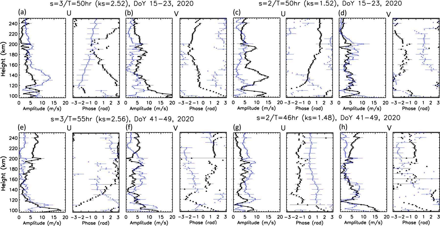
Height profiles of Q2DW_app (black) and Q2DW_eff (blue) amplitudes and phases for U and V at 5° geographic latitude. Top: day of year (DOY) 15–23. Bottom: DOY 41–49. Left: s = 3. Right: s = 2.

Now consider the amplitude and phase profiles of Q2DW+3_eff V in Figure 2b. The corresponding phases show downward progression with height, consistent with upward propagation; however, above 120 km the phase progression slows considerably, and above 200 km phases increase with height. Note that above 140 km, amplitudes increase with height up to ∼190 km, and then decrease with height. These amplitude and phase structures are not consistent with a monochromatic upward-propagating Q2DW+3, which would show monotonically-decreasing amplitudes and phases with height above the peak near 105 km. The data suggest that there are SWs aliasing into the Q2DW+3 fit.

The blue symbols/lines in Figure 2b represent the amplitudes and phases of Q2DW+3_eff. Near 105 km, there is a drastic reduction compared with Q2DW+3_app accompanied by downward phase progression with height, which is consistent with destructive interference between the upward-propagating Q2DW+3 and one or more upward-propagating SWs. A more modest reduction in amplitude persists to about 250 km, accompanied by an increase in phase between 130–160 km, and quasi-constant phase above 160 km. The overall reduction in amplitude compared with Q2DW+3_app and the modifications in phase are also consistent with the presence of SWs. Somewhat similar behavior is seen in the V amplitude and phase profiles for Q2DW+2_app and Q2DW+2_eff for DOY 41–49 (Figure 2h), and the U amplitude profile for Q2DW+3_app and Q2DW+3_eff. In the latter case, the phase of Q2DW+3_app increases with height below 160 km, implying an in-situ source and therefore presence of a SW. There are other situations (e.g., V in Figures 2d and 2f and U in Figure 2g) where the amplitudes of apparent and effective Q2DWs are relatively small, do not differ much, and where phase differences may be inconsequential given the small amplitudes.

The U components of the Q2DW during DOY 15–23 for s = 3 vs. s = 2 (Figures 2a vs. 2c), both of which exhibit a pronounced peak near 130–140 km, make an interesting final comparison. In Figure 2a, q2DW+3_app possesses modest amplitudes (<10 ms⁻¹) and downward phase progression below 180 km, consistent with the vertically-propagating Q2DW that resides in the simulation of Gu et al. (2018). However, Q2DW+3_eff reflects a doubling of amplitudes and a prominent peak near 135 km accompanied by upward phase progression with height. This behavior is consistent with a sizable SW superimposed on Q2DW+3. Conversely, the Q2DW+2_app amplitude of U possesses prominent peaks at 110 and 135 km, and increasing phase with height above 110 km, which suggests aliasing into Q2DW+2 by SWs. And, Q2DW+2_eff reflects substantial reductions in amplitude below about 200 km, consistent with the presence of SWs that destructively interfere with those aliasing into Q2DW+2_app.

To provide a better sense of the extent of SW influences on the low to middle thermospheric dynamics for the Q2DW during DOY 15–23, Figure 3 presents height (96–200 km) versus latitude (0–30°) depictions of U amplitudes corresponding to Figures 2a vs. 2c amplitude and phase comparison just described. The stark contrasts between Q2DW_app and Q2DW_eff below 160 km altitude show that SWs can make a significant and pervasive contribution to the Q2DW-related dynamics in the dynamo region where electric fields that influence the Q2DW F-region response are generated. At higher altitudes, where the Q2DW itself does not directly penetrate, there are winds of order 5–10 ms⁻¹ that must also represent the presence of SWs.

Figure 3.

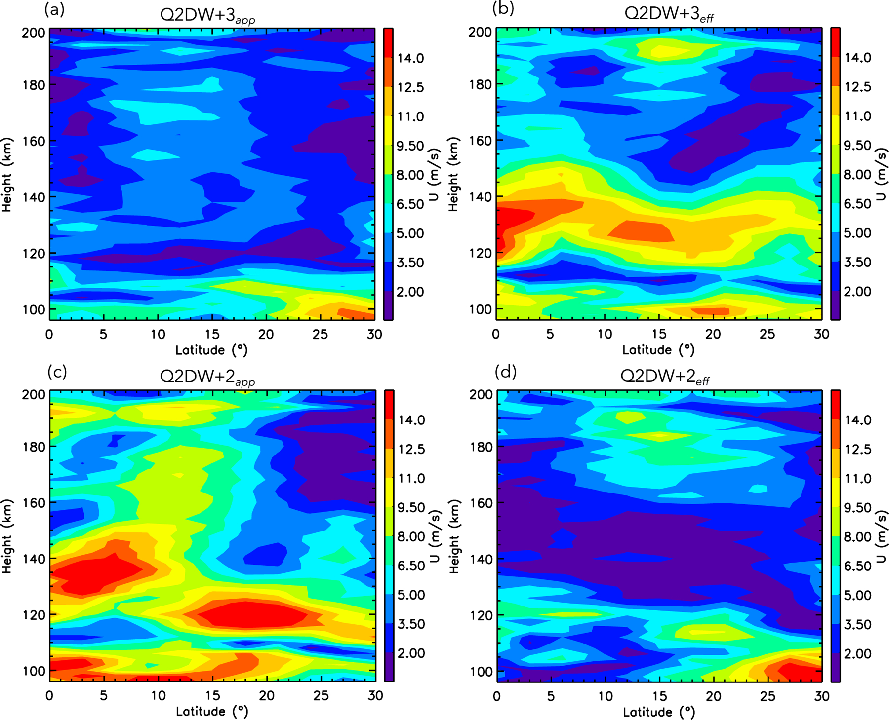
Comparison of apparent (left) and effective (right) Q2DW U amplitudes for s = 3 (top) and s = 2 (bottom) as a function of height and latitude during day of year (DOY) 15–23.

The simulations of Q2DW+3 and its SWs by Gu et al. (2018) and Palo et al. (1999) both yield evidence for 16hW4 and 48hE2 due to its interaction with DW1, and 9.6hW5 and 16hE1 due to its interaction with SW2. However, these model results do not include phase information for SWs, or amplitude information above 140 km (Gu et al., 2018) or 160 km (Palo et al., 1999). Both studies agree that 16hE1 is significantly smaller than the other three SWs. 16hW4 achieves U amplitudes of order 5–15 ms⁻¹ below 140 km over the equator, and extends well into the Northern Hemisphere (∼40^◦ ). This result for 16hW4 is in agreement with results by Chang et al. (2011) and Nguyen et al. (2016) who also report < 5 ms⁻¹ amplitudes for 48hE2. Yue, Wang, et al. (2012) report 6–8 ms⁻¹ amplitudes at 100 km for 16hW4 and also much smaller amplitudes for 48hE2. The 9.6hW5 SW in Gu et al. (2018) and Palo et al. (1999) extends into the 140–160 km height region at amplitudes up to 10 ms⁻¹, and similarly extends well north of the equator. These models differ in details, and the vertical propagation of SWs is dependent on the background wind distribution. Nevertheless, it is clear from a physics-based perspective that the Q2DW+3_app and Q2DW+3_eff amplitudes depicted in Figures 2 and 3 and Figures S1–S8 in Supporting Information S1 plausibly contain significant contributions from SWs.

We furthermore speculate that while Q2DW_app and Q2DW_eff signals in Figures 2 and 3 and Figures S1–S8 in Supporting Information S1 in part reflect vertical extensions of the SWs entering the thermosphere at 100 km, they may also reflect tertiary waves (TWs) resulting from SW interactions with DW1 excited in-situ in the thermosphere, and with SW2 originating below 100 km as well as in-situ. A similar mechanism for secondary excitation of the Q6DW in the thermosphere was proposed by Forbes et al. (2018) and quantitatively shown to be significant by Forbes et al. (2020). Note that in-situ DW1 or SW2 can take the form of winds or ion drag in terms of interactions with SWs. For instance, TWs can be produced as follows: 48hE2 × DW1 → 16hE1 + Q2DW+3 and 48hE2 → × SW2 → 9.6h0 + 16hW4; 16hW → 4 × DW1 → 9.6hW5 + Q2DW+3 and 16hW4 × SW2 → 6.86hW6 + 48hE2; 9.6hW5 × DW1 → 6.86hW6 + 16hW4 and 9.6hW5 × SW2 → 5.33hW7 + Q2DW+3. All of these waves appear as k_s = 2.5. Our reasoning behind this speculation is rooted in the upward phase progressions reflected in Figure 2 and Figures S1–S4 in Supporting Information S1, all of which imply in-situ sources of excitation in the thermosphere. By extrapolation we assume that analogs to all of the above apply for Q2DW+2 and its SWs; however, equivalent numerical simulations for Q2DW+2 do not yet exist.

As one final step in the specification of Q2DW-related neutral dynamics above 100 km, and in preparation for the presentation of plasma drifts in the next subsection, we examine the full reconstructed Q2DW_app or Q2DW_eff wind field that results from superposition of Q2DW+2_app + Q2DW+3_app or Q2DW+2_eff + Q2DW+3_eff, respectively, based on coefficients obtained from the least-squares fittings described in Section 2. Figure 4 shows some depictions of the resulting Q2DW winds for DOY 15–23, and wherein all panels except for Figure 4c correspond to 0° longitude. Figures 4a and 4d illustrate latitude vs. UT plots of total Q2DW_app U amplitudes at 110 km, and V amplitudes at 130 km. (The 110 km altitude is representative of the wind field near the Hall conductivity nominal peak height of 106 km, and 130 km is near the nominal 125 km peak height of the Pedersen conductivity, and thus are most relevant to the dynamo generation of electric fields that produce F-region drifts.) The U winds at 110 km are of order ±13 ms⁻¹ and the V winds are of order ±8.5 ms⁻¹, and thus correspond to ranges of 26 ms⁻¹ and 17 ms⁻¹, respectively. The corresponding latitude vs. LST plots of Q2DW_eff in Figures 4b and 4e reveal ranges of 9 ms⁻¹ and 13 ms⁻¹, and thus significant reductions in comparison to Q2DW_app, at least at these altitudes and 0° longitude. As noted previously, this appears to result from destructive interference of one or more SWs with Q2DW_app. Figure S9 in Supporting Information S1 similarly shows smaller values for Q2DW_eff as compared with Q2DW_app for DOY 41–49. Figure 4c illustrates Q2DW_app U wind speeds (∼±10 ms⁻¹) at 0° latitude as a function of longitude and UT, and Figure 4f illustrates V wind speeds (∼±10 ms⁻¹) as a function of latitude and UT at 0° longitude. F-region meridional winds are relevant to the introduction of Q2DW oscillations in topside Ne at a given height through vertical motions of the F-layer induced by the field-aligned component of V (e.g., Forbes et al., 2018), and through their contributions to interhemispheric transport (Burrell & Heelis, 2012; Burrell et al., 2011, 2013).

Figure 4.

Latitude vs. UT(LST) reconstructions of apparent(effective) Q2DW neutral winds during day of year (DOY) 15–23 and 0° longitude for U (top) and V (bottom) at select heights.

4.2. Radar Wind Measurements Below 100 km

We use the same G-B observations from meteor radars at Peru (77°W, 12°S, Chau et al., 2021), and Cariri (36.5°W, 7.4°S, Lima, et al., 2012), Tirupati (79.4°E, 13.6°N, Rao et al., 2014) and Ledong (109.0°E, 18.4°N, Wang et al., 2019) as in Paper #1. Lomb-Scargle analysis is implemented on radar winds in a 5-day sliding window for each of U and V components at each of the radars. The amplitudes at the periods of 48, 16 and 9.6 h are averaged between 90 and 95 km altitude and displayed in Figure 5. The amplitudes are overall larger in V (Figures 5e–5h) than in U (Figures 5a–5d). In V and at all four radars, the 48 h amplitudes are mostly above the significance level α = 0.05, whereas the 9.6 and 16 h amplitudes are mostly below the significance level. The 48 h oscillation was investigated in Paper #1 in terms of zonal wavenumber, amplitude and its dependences on latitude, frequency, and altitude. In V at the radars at Peru and Cariri (Figures 5g–5h), the 16 h amplitudes are above the significance level occasionally during DOY 25–35. As illustrated by the vertical blue line in Figures 5g–5h, the product of the 16 h V amplitude at Peru with that at Cariri maximizes at DOY 27. Combining the amplitudes at these two radars, we diagnosed that the zonal wavenumber of the underlying 16 h wave at DOY 27 is associated with s = 4, using the technique developed in He et al. (2018). Using the same method and observations, we showed that the 48 h wave is dominated by s = 3 at DOY 5–35 in Figure S2 in Supporting Information S1 in Paper #1. Therefore, the 16 h wave with s = 4, that is, 16hW4, can be explained as the secondary wave of the interaction of Q2DW+3 × DW1.

Figure 5.

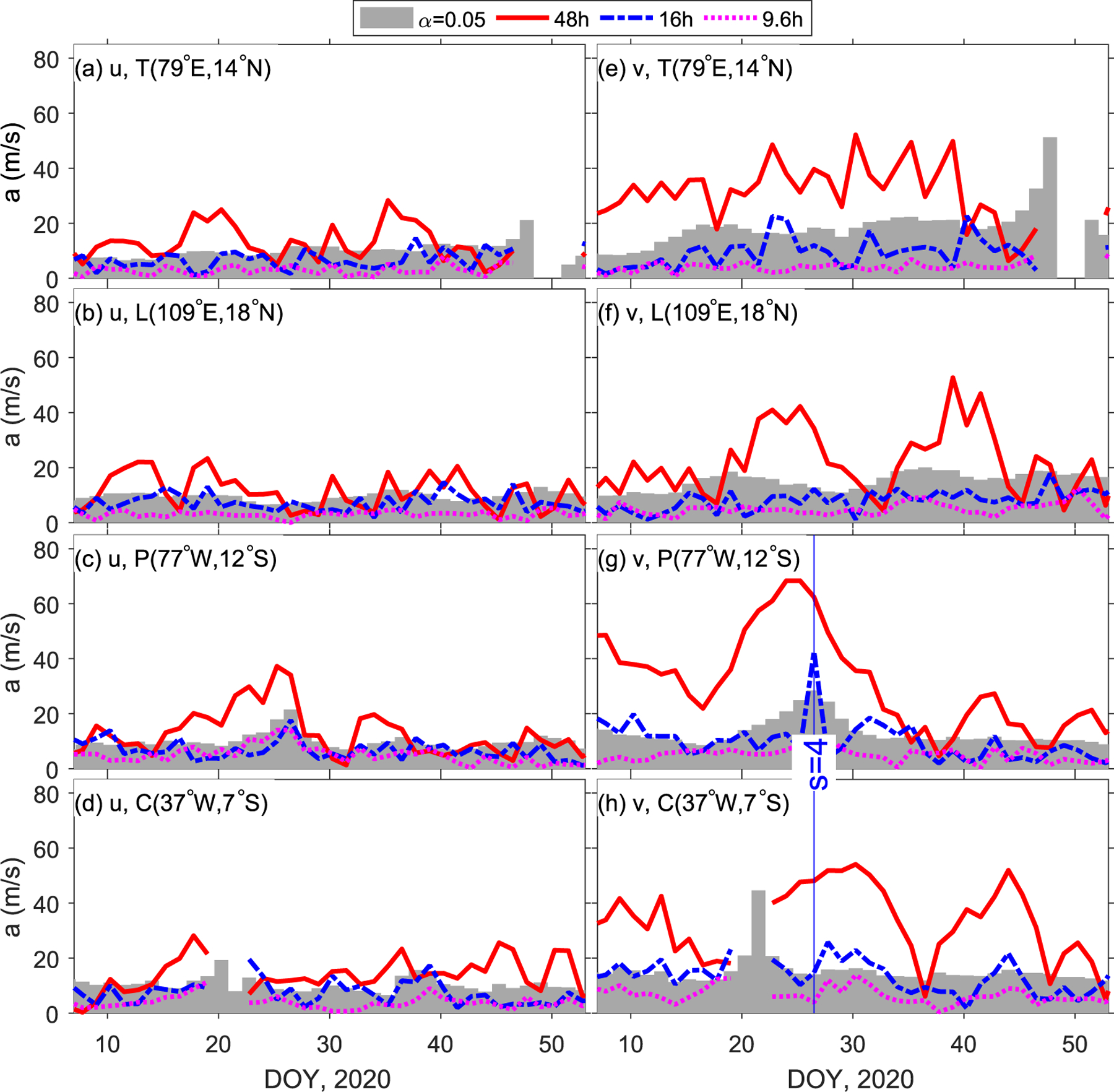
Amplitudes of 48, 16, and 9.6 h oscillations in (a–d) U and (e–h) V at 90–95 km altitude observed by four meteor radars, at Tirupati (T, 79°E, 14°N), Ledong (L, 109°E, 18°N), Peru (P, 77°W, 12°S), and Cariri (C, 37°W, 7°S). In each panel, the gray regions indicate the significance level α = 0.05. In (g) and (h), the blue vertical line indicates the maximum product of the 16 h amplitude in (g) with that in (h) which are used for diagnosing the zonal wavenumber of the underlying 16 h wave.

The significant levels in Figure 5 have a relatively high threshold (≳10 ms⁻¹) in comparison to SW amplitudes at 90–95 km from the models discussed in the previous subsection. For 16hW4 and 9.6hW5, the largest SWs predicted by the models, peak amplitudes occur at or above 100 km, with amplitudes at 90–95 km usually ≤ the 10 ms⁻¹ minimum amplitudes that can be detected with confidence, as indicated in Figure 5.

The comparatively large 16hW4 SW observed on DOY 27 unfortunately fell outside the 4 9-day time intervals available for study of the Q2DW from space in the present study. This leads us to the important conclusion that while SWs may not be readily detectable by specular meteor radars, SWs are capable of assuming significantly larger amplitudes in the dynamo region above. The extent to which such SWs are capable of producing ionospheric effects in the F-region during January-February, 2020, is explored in the following subsections.

4.3. Plasma Drift Q2DW Response

In this subsection the plasma drift response to Q2DW neutral dynamics is presented. Recall that plasma drift data are available for DOY 15–23, but not DOY 41–49. However, given that the measurements presented herein represent the only Q2DW drift measurements that exist to date, and contemporaneous plasma drift and Ne measurements do exist for DOY 35–43, in this section Q2DW drift measurements are presented for both DOY 15–23 and DOY 35–43. From Paper #1, we furthermore know that the Q2DW neutral dynamics during DOY 35–43 more strongly reflects Q2DW+2, whereas DOY 15–23 more strongly reflects the presence of Q2DW+3. It is therefore of interest to ascertain to what degree this difference between time periods is reflected in the drifts.

The drifts measured by ICON during this period occur near 600 km altitude, well above the mean ≲325 km altitude of the F-layer peak as determined from ICON FUV measurements (not shown), as is typical of low latitudes during solar minimum conditions (e.g., Li et al., 2018). The ICON/IVM plasma drift data products include the meridional E × B drift (V_m), which is perpendicular to B within the magnetic meridional plane, and maps to upward vertical drift at the magnetic equator; the field-aligned drift (V_A), which is positive along the main magnetic field vector; and the vertical drift (V_Z), which is positive downward, and consists of contributions from the vertical projections of V_M and V_A at any point along a field line. Since the magnetic field lines are equipotentials, V_M at a given height is symmetric about the equator in magnetic coordinates. V_A and V_Z can be asymmetric about the equator. V_A consists of contributions from field-aligned components of neutral winds, gravity and plasma pressure gradient, and the plasma pressure gradient is in turn affected by ion production and loss at lower altitudes, neutral winds below the F-layer peak, and meridional E × B plasma drifts (Burrell et al., 2011). At the magnetic equator, V_A due to winds and pressure gradients can transport plasma between hemispheres, and at speeds that increase with height as the topside Ne decreases (Burrell & Heelis, 2012; Burrell et al., 2013). In this paper we report on the Q2DW variations in V_M, V_A, V_Z for the first time, and Ne variations in the topside F-region for the first time.

Similar to Figure 1 for MIGHTI winds, Figure 6 provides an example of data coverage for the vertical drifts (V_Z) at the magnetic equator (top) and 12°S magnetic latitude (bottom) in the form of residuals from the zonal mean for DOY 15–23 organized according to sub-divided longitude and UT for s = 2 and s = 3. The coverage at the magnetic equator is typical of other latitudes for both DOY 15–23 and 35–43, with the exception of southward of 12°S for DOY 15–23 and northward of 12°N for DOY 35–43; in these cases the data are spotty and not utilized. An example of “worst case” coverage used to extract the Q2DW is provided in the bottom panels of Figure 6. In this case the data covers 3 cycles of the Q2DW, as opposed to 4.5 cycles when data from all 9 days in the interval are fit. As with the wind data, all of the data points in each panel of Figure 6 are fit in a least-squares sense to obtain a single amplitude and phase every 3° latitude for each of Q2DW+2_app, Q2DW+3_app, Q2DW+2_eff and Q2DW+3_eff for each time period.

Figure 6.

Data coverage of ion velocity meter (IVM) vertical plasma drifts within ±5° of the magnetic equator as a function of subdivided longitude and days during day of year (DOY) 15–23. (a) s = 3 (b) s = 2.

The amplitudes and phases for the fitting just described are provided in Figures 7–10 for V_M, V_A, V_z and Ne, respectively. For reference, magnetic latitude vs. LST plots of zonal-mean values of these parameters averaged over DOY 10–45 (35dZM) are provided in Figure S6 of the Supporting Information S1. As addressed in the following paragraphs, these figures provide a measure of the observed Q2DW responses in these ionospheric parameters that are forced by the neutral winds described in Figure 2, Figures S2–S5 in Supporting Information S1, and in Paper #1; comparisons between Q2DW_app and Q2DW_eff determinations of these ionospheric parameters to assist in evaluating potential SW effects; potential relationships between Q2DW Ne and plasma drifts; and observational constraints and targets for first-principles A-I coupling models.

Figure 7.

Q2DW amplitudes of apparent (black) and effective (blue) V_M are shown as a function of magnetic latitude for s = 3 (left) and s = 2 (right) for DOY 15–23 (top) and DOY 35–43 (bottom). Local solar time ranges of the data that were fit are also shown in the left-hand panels.

Figure 10.

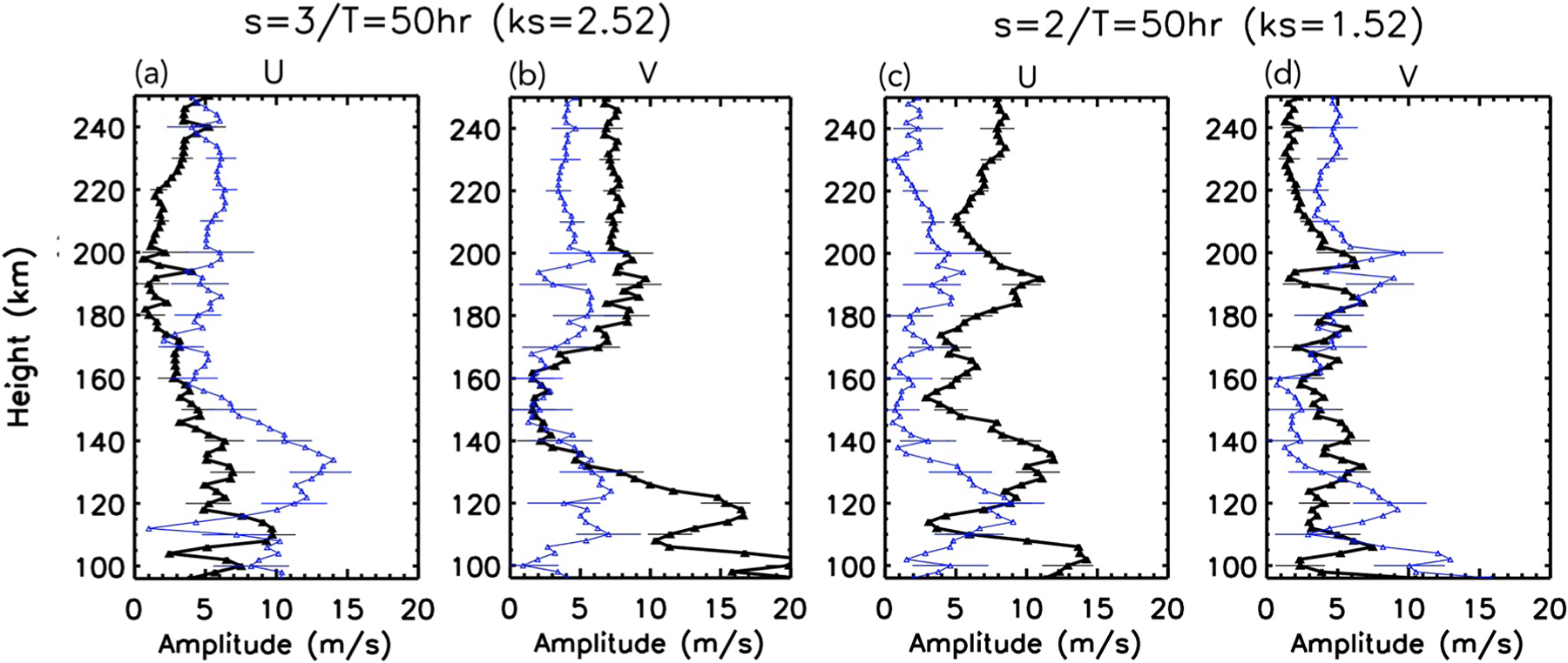
Height profiles of Q2DW_app (black) and Q2DW_eff (blue) amplitudes for U and V at the geographic equator for day of year (DOY) 15–23. Left: s = 3, Right: s = 2.

To get a complete picture, A-I models will need to be sampled in the same way that the IVM instrument samples the ionosphere in order to fully understand the observations presented here. This is particularly evident from Figure 7, where V_M is not symmetric about the equator at all latitudes, as compared with model results that show the vertical component of the Q2DW E × B vertical drift (W_i) to be nearly symmetric about the equator (e.g., Gu, Liu, Li, & Dou, 2015; Yue, Liu, & Chang, 2012). On the other hand, given the relatively large standard deviations in Figure 7, significant asymmetries are not pervasive, especially for the apparent Q2DWs. The inconsistencies with theoretical expectations when they do occur are likely linked to the fact that the two hemispheres are sampled at different LSTs, longitudes and DOY. Moreover, the Q2DW may not be a steady-state (fixed amplitude and period) oscillation. The amplitudes in Figure 7, which range between 1 to 5 ms⁻¹ (as compared with 35dZM values of order 10–40 ms⁻¹), only represent a “best fit” to the collective 7.5–9.0 days of observations, each quasi-2-day cycle being sampled somewhat differently than the others, and at different points within each cycle due to wave period not being exactly 48 h.

The noteworthy aspect of Figure 8 is the relative size of V_A amplitudes (5–25 ms⁻¹) in comparison to the ∼±10 ms⁻¹ neutral winds near 240 km, and to the 35dZM magnitudes of ∼100 ms⁻¹. The 35dZM background drifts contain components due the neutral wind and to the field-aligned plasma pressure gradient, the latter contribution to the drift increasing with height as Ne decreases (Burrell & Heelis, 2012; Burrell et al., 2011, 2013). The neutral wind field is not expected to increase much with height between 240 and 600 km due to the effectiveness of molecular viscosity in preventing significant vertical wind shears from occurring. These factors suggest that the neutral wind at lower altitudes modulates the F-peak height and the associated field-aligned plasma pressure gradient to drive a Q2DW in V_A shown in Figure 8. By analogy with the connection that exists between the background V_A and hemispheric differences in the Ne distribution, there may be a correlation between the Q2DW components of V_A and Ne; this will be explored in the following subsection.

Figure 8.

Same as Figure 7, except for V_A.

Figure 9 presents similar results to Figures 7 and 8 except for V_Z, which contains contributions (projections onto the vertical direction) from V_M and V_A. The V_Z amplitudes generally fall within the 1.0–5.0 ms⁻¹ range, compared to 35dZM values which range between about −90 ms⁻¹ (pre-noon) to +40 ms⁻¹. V_Z is relevant to interpretation of Q2DW variations in Ne, since up and down motions of the F-layer translate directly to increases and decreases in Ne assuming other influences on Ne remain fixed. The striking aspect of Figure 9 is the consistency in latitude shapes and amplitudes (taking into account the standard deviations of the displayed amplitudes) between Q2DW+3_app and Q2DW+3_eff on one hand and Q2DW+2_app and Q2DW+2_eff on the other.

Figure 9.

Same as Figure 7, except for V_Z.

This consistency is also true between Figures 8a, 8c and 8d for V_A, but to a lesser extent for V_M in Figure 7. The one point of consistency in this regard is that panels (b) in Figures 7 and 8 are the ones that reflect the greatest differences between apparent and effective Q2DWs, namely between Q2DW+2_app and Q2DW+2_eff for DOY 15–23, which is the time period for which contemporaneous Q2DW neutral wind and Ne measurements both exist. These connections will be taken up in the following subsection, which focuses on the relationships between Q2DW drifts and Ne.

In terms of numerical simulations, there is not very much that can be directly compared with the results In Figures 7–9. Model results to date have not reported V_A and V_M in the context of the Q2DW, especially in the topside F-region near 600 km, and the concept of effective Q2DWs is introduced for the first time in the present paper. And, there is the additional problem that the simulations that do exist do not replicate the E-region dynamo winds specific to the Q2DW events that occurred during DOY 10–43, 2020. For instance, the Q2DW+2(Q2DW+3) U and V amplitudes of about 30(15) ms⁻¹ and 70(40) ms⁻¹ near their 100-km maxima, respectively, reported by Gu, Liu, Li, and Dou (2015) considerably exceed those reported here; namely, 14(7) ms⁻¹ for U and 12(20) ms⁻¹ for V. The Gu, Liu, Li, and Dou (2015) simulations show that both U and V can make significant contributions to the Q2DW+2 and Q2DW+3 vertical E × B drifts (W_i), that significant latitude structures in W_i can exist which depend on the relative magnitudes and phases of U and V (and also presumably on their height structures relative to Hall and Pedersen conductivities), and that the W_i latitude distributions tend to maximize at middle latitudes with more flat latitude variations within ±20° magnetic latitude. Another relevant conclusion from this modeling work is that winds directly associated with Q2DW+2 and Q2DW+3, as opposed to those associated with their SWs, are each capable of producing vertical drift magnitudes important to F-region variability. This information from modeling can be useful in gaining some insight into the relationship between Q2DW winds and drifts for DOY 15–23. A few examples follow.

First, given that V_M in this latitude range is an approximate measure of W_i, it can be stated that Q2DW+2_app and Q2DW+3_app in Figure 7 do not have pronounced latitude variations, and lie in the range 2.0 ± 1.0 ms⁻¹ for Q2DW+3_app and 4.0 ± 1.0 ms⁻¹ for Q2DW+2_app, as compared with about 1.2 ± 0.2 ms⁻¹ for Q2DW+3_app and 4.2 ± 0.2 ms⁻¹ for Q2DW+2_app (Gu, Liu, Li, & Dou, 2015, their Figure 3). Thus the equatorial-region drifts reflected in the observations and model compare more favorably in magnitude than the those of the 100-km Q2DW winds quoted above, suggesting that a more meaningful comparison might be between the modeled and observed height-integrated conductivity-weighted winds, which are more relevant to the generation of electric fields and drifts. It is also noted that modeling by Yue, Wang, et al. (2012) shows that the Q2DW+3 itself produces equatorial-region W_i of order 1.0 ms⁻¹, in agreement with Gu, Liu, Li, and Dou (2015).

Second, a collective observation that can be drawn from Figures 7–10 is that in most cases the values of the effective Q2DWs do not differ appreciably from the apparent Q2DW, which would be consistent with minimal influence of SWs on the production of plasma drifts. This supports the conclusion of Gu, Liu, Li, and Dou (2015) that winds directly associated with Q2DW+2 and Q2DW+3 are each capable of producing the vertical drift magnitudes quoted above, while at the same time noting that this does not imply that SWs cannot also contribute to the generation of drifts. In a few cases effective and apparent Q2DW amplitudes in Figures 7–9 depart from each other at a few latitudes, while the most pronounced departure between the two occurs during DOY 15–23 for V_M and V_A (Figures 7b and 8b), with Q2DW+2_app significantly exceeding Q2DW+2_eff at almost all latitudes. The reader is referred back to Figures 3 and 3d, which illustrate that the Q2DW+2_eff zonal wind is significantly reduced compared to the Q2DW+2_app zonal wind, and this was interpreted as a destructive interference effect introduced by one or more SWs. The similar response in V_A and V_M suggests a cause-effect relationship involving SWs.

On the other hand, the reverse situation exists between Q2DW+3_app and Q2DW+3_eff in Figures 3a and 3b, but this is not similarly translated to V_M and V_A in Figures 7a and 8a. Drawing on the importance of both U and V in driving plasma drifts learned from the modeling work of Gu, Liu, Li, and Dou (2015), a plausible explanation for this disparity in the drifts is provided in connection with Figure 10. Figure 10 provides vertical profiles similar to those in Figure 2 for DOY 15–23, except at the geographic equator where the effects to be discussed are most prominent (note that vertical profiles for other latitudes are provided in Figures S2 and S5 in Supporting Information S1). If one imagines the height-integrated differences between the blue and black curves (i.e., Q2DW_eff vs. Q2DW_app), then it is clear that Q2DW+3_eff > Q2DW+3_app for U but Q2DW+3_eff < Q2DW+3_app for V, whereas Q2DW+2_eff < Q2DW+2_app for U but Q2DW+2_eff ∼ Q2DW+2_app for V. In the former case, significant SW effects exist, but are acting against each other in terms of driving differences between Q2DW+3_eff and Q2DW+3_app in the drifts (Figure 7a and 8a). In the latter case, differences in U winds between Q2DW+2_eff and Q2DW+2_app are relatively unopposed by similar differences in V winds, leading to the enhanced Q2DW+2_app drifts relative to the Q2DW+2_eff drifts in Figures 7b and 8b.

The above results and interpretations suggest that there are latitude regions and periods of time where and when SWs can exert significant influence on plasma drifts, and this appears to be in line with modeling results that are available. For instance, Yue et al. (2016) show that the individual amplitudes of 16hW4 and 48hE2 equatorial-region W_i to be about 1.2 and 0.2 ms⁻¹, respectively, and Gu et al. (2018) report individual magnitudes of order ±1.0 ms⁻¹ for W_i between LST 1000 and 1600 and ±18° magnetic latitude for 16hW4, 48hE2, and 9.6hW5. However, these authors do not report the combined effects of these SWs in a form that can be compared with the results derived in the present paper. Moreover, no simulations currently exist for SWs produced by Q2DW+2-tide interactions. In the future, it would be very beneficial for modelers to quote values for Q2DW+3_eff in addition to those for its individual contributors, so that such comparisons with S-B determinations of the Q2DW can be made.

We now turn to the Q2DW perturbations in Ne derived from the ICON/IVM measurements and seek to make connections with the plasma drifts just reported.

4.4. Q2DW Ne Responses and Relationships With Drifts

Figure 11 presents the Ne Q2DW amplitudes, calculated from % residuals of Ne from the zonal mean, that correspond to Figures 7–9. It is immediately evident that the larger amplitude of Q2DW+2_app with respect to Q2DW+2_eff in V_M noted above (Figure 7b) are also reflected in Ne (Figures 11b, ∼8%–13% vs. 2%–7%). In addition, the relative structures of Q2DW+3_app vs. Q2DW+3_eff Ne in Figures 11c, with Q2DW+3_app mostly exceeding Q2DW+3_eff, are very similar to those for V_M in Figure 7c, while Q2DW+3_app and Q2DW+3_eff agree with each other within the given uncertainties in both Figure 7a (V_M) and Figures 11a (Ne). Finally the comparison between V_M in Figure 7d and Ne in Figures 11d is interesting. In both cases Q2DW_app has similar latitude structures (maxima in both hemispheres, minimum at 3°S), and the Q2DW_eff’s are near-mirror images of each other.

Figure 11.

Same as Figure 7, except for Ne.

To reveal the full extent of Q2DW variability in drifts and Ne, the amplitudes and phases in Figures 7–9 and are used to perform reconstructions in the form of latitude vs. UT(DOY) plots in Figure 12 for DOY 15–23, and in Figure 13 for DOY 35–43. (Note that this is only possible for apparent Q2DWs where periods and zonal wavenumbers of the waves are known or can be reasonably assumed. By their nature, effective Q2DWs consist of an unknown conglomeration of waves of various periods and zonal wavenumbers, all with a common k_s.) Broadly speaking, for DOY 15–23(DOY 35–43), we can say that ∼±12%(18%) variability in Ne is associated with ±4–5(6–8) ms⁻¹ variability in V_M and V_Z. Also, the in-phase correlation of Ne with V_M and the anti-phase correlation of Ne with V_Z (positive downward) in the NH, are both consistent in sign with changes in Ne that would occur as the result of up and down motions of the F-layer.

Figure 12.

Magnetic latitude vs. DOY Q2DW+3_app + Q2DW + 2_app reconstructions for (a) Ne, (b) V_Z, (c) V_M and (d) V_A for day of year (DOY) 15–23 at 0° longitude.

Figure 13.

Same as Figure 12, except for day of year (DOY) 35–43.

According to Burrell et al. (2013), based on analyses of C/NOFS and GPS occultation data during daytime and solar minimum, V_A > 0 implies a positive conjugate displacement of hmF2 between the SH and NH; namely, hmF2(SH) > hmF2(NH) near ∓15° magnetic latitudes where the magnetic field lines have an apex height ∼600 km. Consistent with the above conclusions drawn on the basis of upward/downward vertical drifts, V_A > 0 at the magnetic equator also implies that Ne(SH) > Ne(NH) near ±15° magnetic, but it is not clear from their analysis to what extent this effect would be visible equatorward of ±15°. V_A is influenced by both meridional winds below the F-layer peak, which act to produce the latitude asymmetry and associated plasma pressure gradient parallel to the magnetic field, and by E × B drift which induces a fountain-effect diffusive motion. Examination of the behavior of the plasma motion in Figures 12 and 13 show that upward(downward) E × B drifts are associated with poleward(equatorward) field-aligned drifts, consistent with the expected diffusive motions. However, the peaks in the field-aligned motions are displaced to the southern hemisphere in both cases. This would require meridional wind induced field-aligned motions that are directed from north to south when the E × B drift is upward and south to north when the E × B drift is downward. The winds at 240 km shown in Figure 4f only partially show a consistent phase relationship with the E × B drifts, and besides, winds at this altitude may not represent the dominant driver of latitudinal asymmetries in the topside plasma density. A complete understanding of the Ne variability in Figures 12a and 13a requires numerical modeling devoted to this topic.

Finally, complementary figures to those just presented for Ne in Figures 11–13, are provided in Figures 14 and 15 for DOY 10–18 and DOY 30–38. The reader is reminded that there are no suitable plasma drifts available for these two 9-day periods. Nevertheless, Figure 14 reinforces previous results in that (a) the effective and apparent Q2DW latitude structures track each other relatively well with sometimes measurable but not profound differences in amplitude; and (b) that the s = +2 Q2DW ionospheric response can be of equal and sometimes greater importance than the s = +3 response, which has received the majority attention in the literature except for the studies of Gu et al. (2016), Gu, Liu, Li, and Dou (2015), and Gu, Liu, Li, and Dou et al. (2015). Figures 14a and 14b and Figure 15 in fact illustrate how destructive interference between Q2DW+2_app and Q2DW+3_app, each of order ≳10% (Figures 14a and 14b, for DOY 10–18), can lead to a relatively small (< 5%) total Ne Q2DW response (e.g., in the NH), but can also combine to produce an Ne response of order ±30% (e.g., Figure 15b for DOY 30–38).

Figure 14.

Same as Figure 11, except for day of year (DOY) 10–18 (top) and DOY 30–38 (bottom).

Figure 15.

Same as Figure 12a, except for (a) day of year (DOY) 10–18 and (b) DOY 30–38.

5. Summary and Conclusions

In Paper #1 (He, Chau et al., 2021) it was demonstrated, using a combination of ICON/MIGHTI and G-B radar measurements, that Q2DW activity during January - March, 2020, was comprised of zonal wavenumber components s = 2 and s = 3 (Q2DW+2 and Q2DW+3). That paper was largely devoted to the temporal evolutions of the Q2DW+2 and Q2DW+3 wind magnitudes and wave periods, and examination of the Q2DW wind field up to 200 km altitude during DOY 15–43 and DOY 41–49 when Q2DW+3 and Q2DW+2, respectively were most prominent.

The present paper is mainly focused on A-I coupling by the Q2DW within several 9-day time periods during the same interval of Q2DW activity as in Paper #1. For DOY 15–23, we utilize ICON measurements to obtain the first contemporaneous measurements of dynamo-region (ca. 100–150 km) Q2DW winds and the F-region ionospheric response in plasma drifts and Ne. This 9-day period is chosen on the basis of coincident coverage of wind and ionospheric measurements during daytime when A-I coupling through the dynamo-generated electric fields is active, and on data quality considerations. Q2DW plasma drifts and Ne are also presented for DOY 35–43, and Q2DW Ne variability is also presented for DOY 10–18 and DOY 30–38 Q2DW. These additional daytime periods of Q2DW coupling are also based on data coverage, data quality, and sampling across various degrees of Q2DW+2 vs. Q2DW+3 forcing. DOY 35–43 is also the first time that Q2DW drifts and Ne have been concurrently measured.

As suggested by recent numerical simulations (e.g., Gu, Liu, Li, Dou, et al., 2015; Gu et al., 2018; Yue et al., 2016), our focus on A-I coupling by the Q2DW necessitates consideration of the potential influences of SWs generated as the result of Q2DW-tide nonlinear interactions. However, it is well-known that the asynchronous nature of S-B measurements introduces special challenges specific to study of the Q2DW, mainly stemming from the fact that the Q2DW period (≈48 h) is a near-integer multiple of solar tidal periods (24, 12 and 8 h). The generated SWs consequently all have periods of 48, 16 and 9.6 h over a range of zonal wavenumbers, both eastward- and westward propagating. Moreover, the Q2DW of a particular wavenumber, and the SWs generated through nonlinear interaction between that Q2DW and all migrating tides, all project onto the same S-B wavenumber, k_s. This means that SWs can alias into the extraction of Q2DW+2 and Q2DW+3 from observational data, and that a given k_s contains contributions not only from the parent Q2DW, but also from all of its SWs.

For ease of presentation, to bring some clarity to the problem, and to enrich our understanding of Q2DWs viewed from space, we adopted the following nomenclatures and perspectives pertaining to Q2DWs. The term “apparent Q2DW” (Q2DW_app) refers to any Q2DW extracted from observational data that potentially contains spatial and/or temporal aliasing contributions from other wave sources. This descriptor applies to all Q2DW determinations determined from S-B data and single-site G-B data published in the literature to date. A “true Q2DW” is one where the methodology for extraction determines both the period and zonal wavenumbers of the Q2DW, that is, as in G-B studies that employ longitudinal chains of instruments (e.g., He, Forbes, et al., 2021; He, Chau et al., 2021; Pancheva et al., 2004; Malinga & Ruohoniemi, 2007; Meek et al., 1996). We also define an “effective Q2DW” (Q2DW_eff) as one obtained by fitting a particular k_s to S-B data, resulting in a quantity that consists of the net contributions of a true Q2DW plus all of its SWs. Q2DW_eff is particularly applicable to the ionospheric response to a Q2DW, since it embodies the net effect of that Q2DW including its SWs, and is in some sense the true ionospheric response to that Q2DW.

Herein we also reported on attempts to detect SWs during January-February, 2020, using winds measured at 90–95 km by four specular meteor radars in the equatorial region. No 9.6 hr SWs rose above the ∼10–20 ms⁻¹ amplitude limits of statistically-significant detectability. Although a few 16 h waves could be detected, only one 16hW4 SW had sufficient longitudinal coherence between radars that its wavenumber could be determined. This result is consistent with available numerical simulations of SWs due to Q2DW-tide interactions (Chang et al., 2011; Gu et al., 2018; Nguyen et al., 2016; Palo et al., 1999; Yue, Liu, & Chang, 2012), which collectively show that the maxima of SWs occur at or above 100 km, with amplitudes at 90–95 being near the radar detectability limits.

However, the same numerical simulations of SWs produced by Q2DW-tide interactions provide some confidence in concluding that SWs were capable of contributing to the Q2DW+2_app, Q2DW+3_app, Q2DW+2_eff and Q2DW+3_eff winds derived from MIGHTI measurements above 100 km, at least to 140–160 km. Features in the vertical profiles between 100 and 250 km such as amplitude and/or phase increases with height, which are inconsistent with that of a vertically-propagating monochromatic Q2DW, were viewed as evidence for the presence of SWs, and moreover, as evidence for the possible in-situ generation of tertiary SWs due to SW interactions with in-situ tides in the thermosphere.

Latitude structures of Q2DW_app and Q2DW_eff s = +2 and s = +3 amplitudes and phases were also constructed for meridional (V_M), field-aligned (V_A) and vertical (V_Z) plasma drifts, and total ion density (\coloneq Ne, electron density). For the most part, the apparent and effective latitude structures of these quantities tracked each other sufficiently well to conclude that the importance of SWs on the ionospheric response were the exception rather than the rule. That being said, there were a few time periods and latitudes where the only possible interpretation was that significant SW influences were present. And, during DOY 15–23 there was a major departure between Q2DW+2_app and Q2DW+2_eff ionospheric responses that was traced back to significant departures between the Q2DW+2_app and Q2DW+2_eff neutral wind profiles.

In addition to amplitudes and phases, the Q2DW responses in this paper were cast in the form of total perturbation reconstructions based on superposition of s = 2 and s = 3 Q2DW components. These reconstructions as functions of latitude, longitude and time are viewed as more informative in terms of actual impacts of the Q2DWs on the thermosphere and ionosphere. In broad terms, we found that the total Q2DW ionospheric responses consist of topside F-region V_A and V_M of order ±25 ms⁻¹ and ±5–7 ms⁻¹, respectively, and Ne perturbations of order (±10%–25%). It is also important to note that the Q2DW s = +2 neutral wind and ionospheric responses in the thermosphere and ionosphere can be just as important as the more widely-studied s = +3 Q2DW responses, although this is likely a function of the particular Q2DW event under study.

Finally, the reader is reminded of the substantial vertical extent of the Q2DW influences and ionospheric processes that are reported here. The Q2DW ionospheric responses noted above are measured near 600 km altitude. The measured Q2DW oscillations in E × B drifts measured at these altitudes result from electric fields generated by neutral wind-plasma interactions nearly 500 km lower, in the ionospheric E-region. It is our interpretation that at intermediate altitudes neutral winds associated with Q2DW SWs can induce latitudinal asymmetries in the plasma pressure gradient parallel to the magnetic field, which combine with the effects of E × B motions to produce the observed field-aligned drifts at ICON altitudes. However, a definitive understanding of the interplay between these processes over the 100–600 km height range in the context of the Q2DW requires numerical simulations devoted to the problem.

Key Points:

• The first contemporaneous measurements of Q2DW winds and the topside ionospheric response are reported based on ICON data

• Q2DW topside F-region field-aligned and meridional drifts of ∼25 m/s and ∼6 m/s, and electron density perturbations of ∼10%–25% occurred

• ICON winds, drifts, Ne, and ground-based radar-measured winds contain signatures of Q2DW-tide nonlinear interactions

Data Availability Statement

The data utilized in this study are available at the ICON data center (https://icon.ssl.berkeley.edu/Data).

References

- Beard AG, Mitchell NJ, Williams PJS, & Kunitake M (1999). Non-linear interactions between tides and planetary waves resulting in periodic tidal variability. Journal of Atmospheric and Solar-Terrestrial Physics, 61, 362–376. [Google Scholar]
- Burrell AG, & Heelis RA (2012). The influence of hemispheric asymmetries on field-aligned ion drifts at the geomagnetic equator. Geophysical Research Letters, 39, L19101. 10.1029/2012GL053637 [DOI] [Google Scholar]
- Burrell AG, Heelis RA, & Ridley A (2013). Daytime altitude variations of the equatorial, topside magnetic field-aligned ion transport at solar minimum. Journal of Geophysical Research: Space Physics, 118, 3568–3575. 10.1002/jgra.50284 [DOI] [Google Scholar]
- Burrell AG, Heelis RA, & Stoneback RA (2011). Latitude and local time variations of topside magnetic field-aligned ion drifts at solar minimum. Journal of Geophysical Research, 116, A11312. 10.1029/2011JA016715 [DOI] [Google Scholar]
- Cevolani G, & Kingsley S (1992). Non-linear effects on tidal and planetary waves in the lower thermosphere: Preliminary results. Advaces in Space Research, 12(10), 77–80. [Google Scholar]
- Chang LC, Palo SE, & Liu H-L (2011). Short-term variability in the migrating diurnal tide caused by interactions with the quasi 2 day wave. Journal of Geophysical Research, 116, D12112. 10.1016/0273-1177(92)90446-5 [DOI] [Google Scholar]
- Chang LC, Yue J, Wang W, Wu Q, & Meier RR (2014). Quasi two day wave-related variability in the background dynamics and composition of the mesosphere/thermosphere, and the ionosphere. Journal of Geophysical Research - Space Physics, 119, 4786–4804. 10.1002/2014JA019936 [DOI] [PMC free article] [PubMed] [Google Scholar]
- Chapman S, & Lindzen RS (1970). Atmospheric tides: Thermal and gravitational (pp. 200). Gordon and Breach. [Google Scholar]
- Chau JL, Urco JM, Vierinen J, Harding BJ, Clahsen M, Pfeffer N, et al. (2021). Multistatic specular meteor radar network in Peru: System description and initial results. Earth and Space Science, 8(1). 10.1029/2020EA001293 [DOI] [Google Scholar]
- Chen P-R (1992). Two-day oscillation of the equatorial ionization anomaly. Journal of Geophysical Research, 97, 6343–6357. [Google Scholar]
- Craig RL, Vincent RA, Fraser GJ, & Smith MH (1980). The quasi-2-day wave in the Southern Hemisphere mesosphere. Nature, 287, 319–320. 10.1038/287319a0 [DOI] [Google Scholar]
- Doyle EM (1968). Wind measurements in the upper atmosphere: PhD thesis, University of Adelaide. [Google Scholar]
- Englert CR, Harlander JM, Brown CM, Marr KD, Miller IJ, Stump JE, et al. (2017). Michelson Interferometer for Global High-resolution Thermospheric Imaging (MIGHTI): Instrument design and calibration. Space Science Reviews, 212, 553–584. 10.1007/s11214-017-0358-4 [DOI] [PMC free article] [PubMed] [Google Scholar]
- Ern M, Preusse P, Kalisch S, Kaufmann M, & Riese M (2013). Role of gravity waves in the forcing of quasi two-day waves in the mesosphere: An observational study. Journal of Geophysical Research Atmospheres, 118, 3467–3485. 10.1029/2012JD018208 [DOI] [Google Scholar]
- Forbes JM, & Moudden Y (2012). Quasi-two-day wave-tide interactions as revealed in satellite observations. Journal of Geophysical Research Space Physics, 117, D12110. 10.1029/2011JD017114 [DOI] [Google Scholar]
- Forbes JM, & Zhang X (2017). The Quasi-6-Day wave and its interactions with solar tides. Journal of Geophysical Research Space Physics, 122, 4764–4776. 10.1002/2017JA023954 [DOI] [Google Scholar]
- Forbes JM, Zhang X, & Maute A (2020). Planetary wave (PW) generation in the thermosphere driven by the PW-modulated tidal spectrum. Journal of Geophysical Research Space Physics, 125, e2019JA027704. 10.1029/2019JA027704 [DOI] [Google Scholar]
- Forbes JM, Zhang X, Maute A, & Hagan ME (2018). Zonally symmetric oscillations of the thermosphere at planetary wave periods. Journal of Geophysical Research: Space Physics, 123, 4110–4128. 10.1002/2018JA025258 [DOI] [Google Scholar]
- Fritts DC, & Isler JR (1994). Mean motion and tidal and two-day structure and variability in the mesosphere and lower thermosphere over Hawaii. Journal of the Atmospheric Sciences, 51, 2145–2164. [Google Scholar]
- Fritts DC, Isler JR, Lieberman RS, Burrage MD, Marsh DR, Nakamura T, et al. (1999). Two-day wave structure and mean flow interactions observed by radar and high resolution doppler imager. Journal of Geophysical Research, 104, 3953–3969. 10.1029/1998jd200024 [DOI] [Google Scholar]
- Gan Q, Oberheide J, Yue J, & Wang W (2017). Short-term variability in the ionosphere due to the nonlinear interaction between the 6-day wave and migrating tides. Journal of Geophysical Research Space Physics, 122, 1–8846. 10.1002/2017JA023947 [DOI] [Google Scholar]
- Garcia RR, Lieberman R, Russell JM, & Mylnczak MG (2005). Large-scale waves in the mesosphere and lower thermosphere observed by SABER. Journal of the Atmospheric Sciences, 62, 4384–4399. 10.1175/JAS3612.1 [DOI] [Google Scholar]
- Gasperini F, Forbes JM, Doornbos EN, & Bruinsma SL (2015). Wave coupling between the lower and middle thermosphere as viewed from TIMED and GOCE. Journal of Geophysical Research Space Physics, 120, 1–5804. 10.1002/2015JA021300 [DOI] [Google Scholar]
- Gu S-Y, Li T, Dou X, Wu Q, Mlynczak MG, & Russell JM (2013). Observations of quasi-two-day wave by TIMED/SABER and TIMED/TIDI. Journal of Geophysical Research Atmospheres, 118, 1624–1639. 10.1002/jgrd.50191 [DOI] [Google Scholar]
- Gu S-Y, Liu H-L, Dou X, & Jia M (2018). Ionospheric variability due to tides and Quasi-two day wave interactions. Journal of Geophysical Research Space Physics, 123, 1554–1565. 10.1002/2017JA025105 [DOI] [Google Scholar]
- Gu S-Y, Liu H-L, Li T, & Dou X (2015). Ionospheric vertical plasma drift perturbations due to the quasi 2 day wave. Journal of Geophysical Research Space Physics, 120, 3941–3948. 10.1002/2015JA021029 [DOI] [Google Scholar]
- Gu S-Y, Liu H-L, Li T, Dou X, Wu Q, & Russell JM III. (2015). Evidence of nonlinear interaction between quasi 2 day wave and quasi-stationary wave. Journal of Geophysical Research Space Physics, 120, 1256–1263. 10.1002/2014JA020919 [DOI] [Google Scholar]
- Gu S-Y, Liu H-L, Pedatella NM, Dou X, Li T, & Chen T (2016). The quasi 2 day wave activities during 2007 austral summer period as revealed by Whole Atmosphere Community Climate Model. Journal of Geophysical Research Space Physics, 121, 2743–2754. 10.1002/2015JA022225 [DOI] [Google Scholar]
- Gu S-Y, Liu H-L, Pedatella NM, Dou X, & Liu Y (2017). On the wave number 2 eastward propagating quasi 2 day wave at middle and high latitudes. Journal of Geophysical Research Space Physics, 122, 4489–4499. 10.1002/2016JA023353 [DOI] [Google Scholar]
- Gurubaran S, Sridharan S, Ramkumar TK, & Rajaram R (2001). The mesospheric quasi-2-day wave over Tirunelveli (8.7N). Journal of Atmospheric and Solar-Terrestrial Physics, 63, 975–985. 10.1016/S1364-6826(01)00016-5 [DOI] [Google Scholar]
- Hagan ME, Forbes JM, & Vial F (1993). Numerical investigations of the propagation of the quasi-two-day wave into the lower thermosphere. Journal of Geophysical Research, 98, 23193–23205. 10.1029/93jd02779 [DOI] [Google Scholar]
- Harding BJ, Chau JL, He M, Englert CR, Harlander JM, Marr KD, et al. (2021). Validation of ICON-MIGHTI thermospheric wind observations: 2. Green-line comparisons to specular meteor radars. Journal of Geophysical Research: Space Physics, 126, e2020JA028947. 10.1029/2020JA028947 [DOI] [PMC free article] [PubMed] [Google Scholar]
- Harding BJ, Makela JJ, Englert CR, Marr KD, Harlander JM, England SL, et al. (2017). The MIGHTI wind retrieval algorithm: Description and verification. Space Science Reviews, 212, 585–600. 10.1007/s11214-017-0359-3 [DOI] [PMC free article] [PubMed] [Google Scholar]
- Harris TJ, & Vincent RA (1993). The quasi-2-day wave observed in the equatorial middle atmosphere. Journal of Geophysical Research, 98, 10,481–10,490. [Google Scholar]
- He M, Chau JL, Forbes JM, Zhang X, Englert CR, Harding BJ, et al. (2021). Quasi-2-day wave in low-latitude atmospheric winds as viewed from the ground and space during January–March, 2020. Geophysical Research Letters, 48, e2021GL093466. 10.1029/2021GL093466 [DOI] [Google Scholar]
- He M, Chau JL, Stober G, Li G, Ning B, & Hoffmann P (2018). Relations between semidiurnal tidal variants through diagnosing the zonal wavenumber using a phase differencing technique based on two ground-based detectors. Journal of Geophysical Research: Atmospheres, 123(8), 4015–4026. 10.1002/2018JD028400 [DOI] [Google Scholar]
- He M, Forbes JM, Li G, Jacobi C, & Hoffmann P (2021). Mesospheric Q2DW interactions with four migrating tides at 53°N latitude: Zonal wavenumber identification through dual-station approaches. Geophysical Research Letters, 48, e2020GL092237. 10.1029/2020GL092237 [DOI] [Google Scholar]
- Heelis RA, Stoneback RA, Perdue MD, Depew MD, Morgan WA, Mankey MW, et al. (2017). Ion velocity measurements for the ionospheric connections explorer. Space Science Reviews, 212, 615–629. 10.1007/s11214-017-0383-3 [DOI] [PMC free article] [PubMed] [Google Scholar]
- Huang KM, Liu AZ, Lu X, Li Z, Gan Q, Gong Y, et al. (2013). Nonlinear coupling between quasi 2 day wave and tides based on meteor radar observations at Maui. Journal of Geophysical Research, 118, 10,936–10,943. 10.1002/jgrd.50872 [DOI] [Google Scholar]
- Huang KM, Liu AZ, Zhang SD, Yi F, Huang CM, Gan Q, et al. (2013). A nonlinear interaction event between a 16-day wave and a diurnal tide from meteor radar observations. Annales Geophysicae, 31, 2039–2048. 10.5194/angeo-31-2039-2013 [DOI] [Google Scholar]
- Huang Y, Zhang S, Yi F, Huang CM, Huang KM, Gan Q, et al. (2013). Global climatological variability of quasi-two-day waves revealed by TIMED/SABER observations. Annales Geophysicae, 31, 1061–1075. 10.5194/angeo-31-1061-2013 [DOI] [Google Scholar]
- Immel TJ, England SL, Mende SB, Heelis RA, Englert CR, Edelstein J, et al. (2018). The ionospheric connection explorer mission: Mission goals and design. Space Science Reviews, 214, 13. 10.1007/s11214-017-0449-2 [DOI] [PMC free article] [PubMed] [Google Scholar]
- Ito R, Karo S, & Tsuda T (1986). Consideration of an ionospheric wind dynamo driven by a planetary wave with a two-day period. Journal of Atmospheric and Solar-Terrestrial Physics, 48(1), 1–13. [Google Scholar]
- Kamalabadi F, Forbes JM, Makarov NA, & Portnyagin Yu. I. (1997). Evidence for nonlinear coupling of planetary waves and tides in the Antarctic mesopause. Journal of Geophysical Research, 102, 4437–4446. [Google Scholar]
- Li K-F, Lin L-C, Bui X-H, & Liang M-C (2018). The 11 year solar cycle response of the equatorial ionization anomaly observed by GPS radio occultation. Journal of Geophysical Research: Space Physics, 123, 848–861. 10.1002/2017JA024634 [DOI] [Google Scholar]
- Lieberman RS (1999). Eliassen–Palm Fluxes of the 2-day wave, Journal of the Atmospheric Sciences, 56, 2846–2861. [DOI] [Google Scholar]
- Lieberman RS, Riggin DM, Nguyen V, Palo SE, Siskind DE, Mitchell NJ, et al. (2017). Global observations of 2 day wave coupling to the diurnal tide in a high-altitude forecast-assimilation system. Journal of Geophysical Research: Atmospheres, 122, 4135–4149. 10.1002/2016JD025144 [DOI] [Google Scholar]
- Lima LM, Alves EO, Batista PP, Clemesha BR, Medeiros AF, & Buriti RA (2012). Sudden stratospheric warming effects on the mesospheric tides and 2-day wave dynamics at 7S. Journal of Atmospheric and Solar-Terrestrial Physics, 78, 99–107. 10.1016/j.jastp.2011.02.013 [DOI] [Google Scholar]
- Lima LM, Batista PP, Takahashi H, & Clemesha BR (2004). Quasi-two-day observed by meteor radar at 22.71S. Journal of Atmospheric and Solar-Terrestrial Physics, 66, 529–537. [Google Scholar]
- Limpasuvan V, & Wu DL (2009). Anomalous two-day wave behavior during the 2006 austral summer. Geophysical Research Letters, 36, L04807. 10.1029/2008GL036387 [DOI] [Google Scholar]
- Limpasuvan V, Wu DL, Schwartz MJ, Waters JW, Wu Q, & Killeen TL (2005). The two-day wave in EOS MLS temperature and wind measurements during 2004–2005 winter. Geophysical Research Letters, 32, L17809. 10.1029/2005GL023396 [DOI] [Google Scholar]
- Makela JJ, Baughman M, Navarro LA, Harding BJ, Englert CR, Harlander JM, et al. (2021). Validation of ICON-MIGHTI thermospheric wind observations: 1. Nighttime Red-line Ground-Based Fabry-Perot Interferometers. Journal of Geophysical Research: Space Physics, 126. 10.1029/2020JA028726 [DOI] [PMC free article] [PubMed] [Google Scholar]
- Malinga SB, & Ruohoniemi JM (2007). The quasi-two-day wave studied using the Northern Hemisphere SuperDARN HF radars. Annales Geophysicae, 25, 1767–1778. 10.5194/angeo-25-1767-2007 [DOI] [Google Scholar]
- McCormack JP, Coy L, & Hoppel KW (2009). Evolution of the quasi 2-day wave during January 2006. Journal of Geophysical Research, 114, D20115. 10.1029/2009JD012239 [DOI] [Google Scholar]
- McCormack JP, Eckermann SD, Hoppel KW, & Vincent RA (2010). Amplification of the quasi-two day wave through nonlinear interaction with the migrating diurnal tide. Geophysical Research Letters, 37, L16810. 10.1029/2010GL043906 [DOI] [Google Scholar]
- Meek CE, Manson AH, Franke SJ, Singer W, Hoffmann P, Clark RR, et al. (1996). Global study of Northern Hemisphere quasi-2-day wave events in recent summers near 90 km altitude. Journal of Atmospheric and Solar-Terrestrial Physics, 58, 1401–1411. 10.1016/0021-9169(95)00120-4 [DOI] [Google Scholar]
- Miyoshi Y, & Yamazaki Y (2020). Excitation mechanism of ionospheric 6-day oscillation during the 2019 September sudden stratospheric warming event. Journal of Geophysical Research Space Physics, 125, e2020JA028283. 10.1029/2020JA028283 [DOI] [Google Scholar]
- Moudden Y, & Forbes JM (2014). Quasi-two-day wave structure, interannual variability, and tidal interactions during the 2002–2011 decade. Journal of Geophysical Research - D: Atmospheres, 119, 2241–2260. 10.1002/2013JD020563 [DOI] [Google Scholar]
- Müller H, & Kingsley S (1974). Long period meteor wind oscillations. Journal of Atmospheric and Solar-Terrestrial Physics, 36, 1933–1943. [Google Scholar]
- Müller H, & Nelson L (1978). A travelling quasi-two-day wave in the meteor region. Journal of Atmospheric and Solar-Terrestrial Physics, 40, 761–766. [Google Scholar]
- Müller HG (1972). A discussion on D and E region winds over Europe-Long-period meteor wind oscillations. Philosophical Transactions of the Royal Society of London - Series A: Mathematical and Physical Sciences, 271(1217), 585–599. 10.1098/rsta.1972.0026 [DOI] [Google Scholar]
- Nguyen VA, Palo SE, Lieberman RS, Forbes JM, Ortland DA, & Siskind DE (2016). Generation of secondary waves arising from nonlinear interaction between the quasi 2 day wave and the migrating diurnal tide. Journal of Geophysical Research Atmospheres, 121, 7762–7780. 10.1002/2016JD024794 [DOI] [Google Scholar]
- Norton WA, & Thuburn J (1996). The two-day wave in a middle atmosphere GCM. Geophysical Research Letters, 23, 2113–2116. 10.1029/96GL01956 [DOI] [Google Scholar]
- Nystrom V, Gasperini F, Forbes JM, & Hagan ME (2018). Exploring wave-wave interactions in a general circulation model. Journal of Geophysical Research Space Physics, 123, 827–847. 10.1002/2017JA024984 [DOI] [Google Scholar]
- Palo SE, & Avery SK (1995). Observations of the meridional quasi-two-day wave in the mesosphere and lower thermosphere at Christmas Island. In The upper mesosphere and lower thermosphere: A review of experiment and theory. Geophysical Monograph Series (Vol. 87, pp. 101–110). American Geophysical Union. [Google Scholar]
- Palo SE, Roble RG, & Hagan ME (1999). Middle atmosphere effects of the quasi-two day wave from a general circulation model. Earth Planets and Space, 51, 629–647. [Google Scholar]
- Pancheva D (1988). Traveling quasi-two-day fluctuations in the summer F-region. Comptes Rendus de l’Academie Bulgare des Sciences, 41, 41–44. [Google Scholar]
- Pancheva D (2006). Quasi-2-day wave and tidal variability observed over Ascension Island during January/February 2003. Journal of Atmospheric and Solar-Terrestrial Physics, 68, 390–407. 10.1016/j.jastp.2005.02.028 [DOI] [Google Scholar]
- Pancheva D, Beard AG, Mitchell NJ, & Muller HG (2000). Nonlinear interactions between planetary waves in the mesosphere lower thermosphere region. Journal of Geophysical Research, 105, 157–170. [Google Scholar]
- Pancheva D, & Lysenko I (1988). Quasi two-day fluctuations observed in the summer F region electron maximum. Bulgarian Geophysical Journal, 14, 41–51. [Google Scholar]
- Pancheva D, Merzlyakov E, Mitchell NJ, Portnyagin Y, Manson AH, Jacobi C, et al. (2002). Global-scale tidal variability during the PSMOS campaign on June-August 1999: Interaction with planetary waves. Journal of Atmospheric and Solar-Terrestrial Physics, 64, 1865–1896. [Google Scholar]
- Pancheva D, & Mitchell NJ (2004). Planetary waves and variability of the semidiurnal tide in the mesosphere and lower thermosphere over Esrange (68°N, 21°E) during winter. Journal of Geophysical Research, 109, A08307. 10.1029/2004JA010433 [DOI] [Google Scholar]
- Pancheva D, Mitchell NJ, Manson AH, Meek CE, Jacobi C, Portnyagin Y, et al. (2004). Variability of the quasi-2-day wave observed in the MLT region during the PSMOS campaign of June-August 1999. Journal of Atmospheric and Solar-Terrestrial Physics, 66, 539–565. 10.1016/j.jastp.2004.01.008 [DOI] [Google Scholar]
- Pancheva D, Mukhtarov P, Siskind DE, & Smith AK (2016). Global distribution and variability of quasi 2 day waves based on the NOGAPS-ALPHA reanalysis model. Journal of Geophysical Research Space Physics, 121, 11,422–11,449. 10.1002/2016JA023381 [DOI] [Google Scholar]
- Pancheva D, Mukhtarov P, & Suskind DE (2018). Climatology of the quasi-2-day waves observed in the MLS/Aura measurements (2005–2014). Journal of Atmospheric and Solar-Terrestrial Physics, 171, 210–224. 10.1016/j.jastp.2017.05.002 [DOI] [Google Scholar]
- Pedatella NM, & Forbes JM (2012). The quasi 2 day wave and spatial-temporal variability of the OH emission and ionosphere. Journal of Geophysical Research Space Physics, 117, A01320. 10.1029/2011JA017186 [DOI] [Google Scholar]
- Pfister L (1985). Baroclinic instability of easterly jets with applications to the summer mesosphere. Journal of the Atmospheric Sciences, 42(4), 313–330. 10.1175/1520-0469(1985)0420313:BIOEJW2.0.CO;2 [DOI] [Google Scholar]
- Plumb RA (1983). Baroclinic instability of the summer mesosphere: A mechanism for the quasi-two-day wave? Journal of the Atmospheric Sciences, 40(1), 262–270. 10.1175/1520-0469(1983)0400262:BIOTSM2.0.CO;2 [DOI] [Google Scholar]
- Raghava Reddi C, Geetha A, & Lekshmi KR (1988). Quasi-2-day wave in the middle atmosphere over Trivandrum. Annales Geophysicae, 6, 231–238. [Google Scholar]
- Randel WJ (1994). Observations of the 2-day wave in NMC stratospheric analyses. Journal of the Atmospheric Sciences, 51(2), 306–313. [DOI] [Google Scholar]
- Rao SVB, Eswaraiah S, Venkat Ratnam M, Kosalendra E, Kishore Kumar K, Sathish Kumar S, et al. (2014). Advanced meteor radar installed at Tirupati: System details and comparison with different radars. Journal of Geophysical Research Space Physics, 119(21), 11,893–11,904. 10.1002/2014JD021781 [DOI] [Google Scholar]
- Rodgers CD, & Prata AJ (1981). Evidence for a travelling 2-day wave in the middle atmosphere. Journal of Geophysical Research, 86, 9661–9664. 10.1029/JC086iC10p09661 [DOI] [Google Scholar]
- Rüster R (1994). VHF radar observations of nonlinear interactions in the summer polar mesosphere. Journal of Atmospheric and Solar-Terrestrial Physics, 56, 1289–1299. [Google Scholar]
- Salby ML (1981). Rossby normal modes in nonuniform background configurations. Part II: Equinox and solstice conditions. Journal of the Atmospheric Sciences, 38, 1827–1840. [Google Scholar]
- Salby ML (1982). Sampling theory for asynoptic satellite observations. Part I: Space-time spectra, resolution, and aliasing. Journal of the Atmospheric Sciences, 39, 2577–2600. [Google Scholar]
- Salby ML, & Callaghan PF (2000). Seasonal amplification of the 2-day wave: Relationship between normal mode and instability. Journal of the Atmospheric Sciences, 58, 1858–1969. [Google Scholar]
- Salby ML, & Roper RG (1980). Long-period oscillations in the meteor region. Journal of the Atmospheric Sciences, 37, 237–244. 10.1175/1520-0469(1980)0370237:LPOITM2.0.CO;2 [DOI] [Google Scholar]
- Teitelbaum H, & Vial F (1991). On tidal variability induced by nonlinear interaction with planetary waves. Journal of Geophysical Research, 96(14), 14,169–14,178. 10.1029/91JA01019 [DOI] [Google Scholar]
- Thayaparan T, Hocking WK, & MacDougall J (1997). Amplitude, phase and period variations of the quasi-2-day wave in the mesosphere and lower thermosphere over London, Canada (43N, 81W), during 1993 and 1994. Journal of Geophysical Research, 102, 9461–9478. 10.1029/96JD03869 [DOI] [Google Scholar]
- Tunbridge VM, Sandford DJ, & Mitchell NJ (2011). Zonal wave numbers of the summertime 2 day planetary wave observed in the mesosphere by EOS Aura Microwave Limb Sounder. Journal of Geophysical Research, 116, D11103. 10.1029/2010JD014567 [DOI] [Google Scholar]
- Wang JC, Chang LC, Yue J, Wang W, & Siskind DE (2017). The quasi 2 day wave response in TIME-GCM nudged with NOGAPS-ALPHA. Journal of Geophysical Research Space Physics, 122, 5709–5732. 10.1002/2016JA023745 [DOI] [Google Scholar]
- Wang Y, Li G, Ning B, Yang S, Sun W, & Yu Y (2019). All-sky interferometric meteor radar observations of zonal structure and drifts of low- latitude ionospheric E region irregularities. Earth and Space Science, 6(12), 2653–2662. 10.1029/2019EA000884 [DOI] [Google Scholar]
- Ward WE, Yang DY, Solheim BH, & Shepherd GG (1996). Observations of the 2-day wave in WINDII data during January 1993. Geophysical Research Letters, 23, 2923–2926. 10.1029/96GL02897 [DOI] [Google Scholar]
- Wu DL, Hays PB, Skinner WR, Marshall AR, Burrage MD, Lieberman RS, et al. (1993). Observations of the quasi-2-day wave from the high resolution Doppler imager. Geophysical Research Letters, 20, 2853–2856. 10.1029/93GL03008 [DOI] [Google Scholar]
- Xu J, Smith AK, Liu M, Liu X, Gao H, Jiang G, & Yuan W (2014). Evidence for nonmigrating tides produced by the interaction between tides and stationary planetary waves in the stratosphere and lower mesosphere. Journal of Geophysical Research Atmospheres, 119, 471–489. 10.1002/2013JD020150 [DOI] [Google Scholar]
- Yue J, Liu H-L, & Chang LC (2012). Numerical investigation of the quasi 2 day wave in the mesosphere and lower thermosphere. Journal of Geophysical Research Space Physics, 117, D05111. 10.1029/2011JD016574 [DOI] [Google Scholar]
- Yue J, Wang W, Richmond AD, & Liu H-L (2012). Quasi-two-day wave coupling of the mesosphere and lower thermosphere-ionosphere in the TIME-GCM: Two-day oscillations in the ionosphere. Journal of Geophysical Research Space Physics, 117, A07305. 10.1029/2012JA017815 [DOI] [Google Scholar]
- Yue J, Wang W, Ruan H, Chang L, & Lei J (2016). Impact of the interaction between the quasi-2 day wave and tides on the ionosphere and thermosphere. Journal of Geophysical Research Space Physics, 121, 3555–3563. 10.1002/2016JA022444 [DOI] [Google Scholar]
- Zhou QH, Sulzer MP, & Tepley CA (1997). An analysis of tidal and planetary waves in the neutral winds and temperature observed at low-latitude E region heights. Journal of Geophysical Research, 102, 11491–11505. 10.1029/97JA00440 [DOI] [Google Scholar]
Associated Data
This section collects any data citations, data availability statements, or supplementary materials included in this article.
Supplementary Materials