A Generative Modeling Approach to Calibrated Predictions: A Use Case on Menstrual Cycle Length Prediction

Abstract

We explore how to quantify uncertainty when designing predictive models for healthcare to provide well-calibrated results. Uncertainty quantification and calibration are critical in medicine, as one must not only accommodate the variability of the underlying physiology, but adjust to the uncertain data collection and reporting process. This occurs not only on the context of electronic health records (i.e., the clinical documentation process), but on mobile health as well (i.e., user specific self-tracking patterns must be accounted for). In this work, we show that accurate uncertainty estimation is directly relevant to an important health application: the prediction of menstrual cycle length, based on self-tracked information. We take advantage of a flexible generative model that accommodates under-dispersed distributions via two degrees of freedom to fit the mean and variance of the observed cycle lengths. From a machine learning perspective, our work showcases how flexible generative models can not only provide state-of-the art predictive accuracy, but enable well-calibrated predictions. From a healthcare perspective, we demonstrate that with flexible generative models, not only can we accommodate the idiosyncrasies of mobile health data, but we can also adjust the predictive uncertainty to per-user cycle length patterns. We evaluate the proposed model in real-world cycle length data collected by one of the most popular menstrual trackers worldwide, and demonstrate how the proposed generative model provides accurate and well-calibrated cycle length predictions. Providing meaningful, less uncertain cycle length predictions is beneficial for menstrual health researchers, mobile health users and developers, as it may help design more usable mobile health solutions.

1. Introduction

One of the primary challenges in predictive modeling for healthcare pertains to handling the uncertainty of both the task and the data at hand, as well as ensuring calibration of model output (Han et al., 2011; Rogers and Walker, 2016; Chen et al., 2020). Because users of these models make decisions —that have health and ethical implications (Gillon, 1994; Siebert, 2003)— based on such predictive outputs, it is critical to ensure users can assess the confidence of a model in its predictions.

In machine learning predictions, different types of uncertainty are entangled. The uncertainty, given a finite amount of data, of a machine learning technique can be captured with the statistical characterization of its predictions, i.e., via the predictive distribution p(y|x) of the model output y given the input features x. Entangled in this predictive distribution are both aleatoric and epistemic uncertainties. The former denotes the randomness inherent in the data generating process, i.e., the observed data (e.g., collected features and observed outcomes). The latter —also known as model uncertainty— reflects the uncertainty of a model’s appropriateness to fit the underlying data generating mechanism.

A goal of statistical machine learning is to devise suitable measures of the uncertainty associated with model predictions (Gneiting et al., 2007). Predictions are probabilistic in nature, taking the form of probability distributions over future events of interest (Dawid, 1984). In a Bayesian view of predictive modeling, the outcome Y, the input features X, and the parameters of a model are viewed as random variables¹. The distributional assumptions over the model class and the uncertainty over parameters can be characterized with priors and incorporated into the predictive distribution via marginalization of such (parametric) model uncertainties, i.e., $p(Y\mid x)={\int }_{\theta }p(Y\mid x,\theta )p(\theta \mid \mathcal{D})\text{d}\theta$, where $\mathcal{D}$ refers to previously observed data.

Within this probabilistic view of prediction, where the predictive distribution characterizes all the uncertainty in the outcome of interest Y, a model’s calibration is a crucial aspect. Calibration refers to the statistical consistency between the distributional forecasts (i.e., the predictive distribution) and the true observations (i.e., the data). As originally argued by Dawid (1984) and many after (Diebold and Mariano, 2002), the predictive posterior must be assessed on the basis of the predicted-observation pairs.

A statistical method is calibrated when, for all the observed examples x for which it predicts an outcome Y = y with probability p(Y = y|x) = p′, the proportion (frequency) of real examples observed for outcome y is equal to p′, across all values of P(Y = y|x). In this sense, calibration is inherently frequentist, but Bayesian views of calibration have also been argued for (Dawid, 1982). Essentially, calibration is concerned with measuring the over-confidence and under-confidence of a statistical model. As such, it helps assess the extent to which a user can trust the model’s predicted outcome probabilities.

In healthcare, the role of uncertainty estimation and model calibration is gaining momentum (Vach, 2013; Calster et al., 2016; Alba et al., 2017; Stevens and Poppe, 2020; Goldstein et al., 2021), partly due to the increase in popularity of deep learning based approaches (Rajkomar et al., 2018). Recent evidence suggests that deep-learning approaches lack calibrated outputs (Guo et al., 2017; Nixon et al., 2019), even if several techniques have been proposed to assess and fix this gap (Dusenberry et al., 2020; Kwon et al., 2020).

Most of the healthcare model calibration work so far is on classification tasks in the context of clinical, electronic health record data. On the contrary, the use case for this work is menstrual cycle length prediction from mobile health data. Based on a user’s self-tracked data from a period tracking app, we aim at forecasting their upcoming cycle length, i.e., the date of their next period. This use case differs from previous work in quantifying uncertainty: (i) we target regression (i.e., next cycle length prediction) rather than classification, and (ii) we leverage mobile health (mHealth) data —subject to self-tracking artifacts, like varying adherence to tracking.

When characterizing and predicting menstrual patterns based on mHealth data, the relevance of uncertainty quantification is two-fold. On the one hand, self-tracked data from mHealth apps reflects both physiological menstrual patterns and user engagement dynamics (Li et al., 2020). Therefore, one must disentangle the uncertainty of the physiological process (i.e., the menstrual cycle) from the uncertainty on the observed data (i.e., whether users track their period). On the other, uncertain predictions in mHealth often result in non-actionable insights, e.g., “your next period will occur within the next two weeks” (Orchard, 2019; Fox and Epstein, 2020).

We hereby operate within a generative modeling framework, and leverage advances in the statistical characterization of complex distributions to accommodate both self-tracking artifacts and cycle length variability (Li et al., 2020). Precisely, we take advantage of probabilistic machine learning (Chen et al., 2020) and devise a flexible generative model that can accommodate the uncertainties of the task at hand and address predictive calibration directly. We demonstrate how to overcome the over-dispersion of Poisson distributed predictions by proposing a Generalized Poisson based model that provides accurate and better calibrated individualized cycle length predictions. Less uncertain cycle length predictions are intrinsically beneficial, and we hypothesize they may also help design better menstrual mHealth solutions, ultimately increasing their usability.

Generalizable Insights about Machine Learning in the Context of Healthcare

This work contributes to machine learning in the context of healthcare by first proposing a flexible generative model to provide accurate and well-calibrated predictions. We demonstrate that our model outperforms black-box neural network and state-of-the-art alternatives, by providing interpretable, accurate and well-calibrated predictions. Armed with well-calibrated predictions, users can trust and act upon predictions with more confidence. Second, we argue for the use of probabilistic modeling in healthcare (Chen et al., 2020), since interpretability, accuracy and uncertainty quantification are critical in the medical domain. More broadly, we advocate for the machine learning in healthcare community to not only focus on point estimate based metrics, but to incorporate the calibration tool-set presented here into the evaluation pipeline.

2. Related Work

Calibration in Predictive Models.

A key endeavor of predictive modeling is to provide forecasts that appropriately quantify uncertainty (Gneiting et al., 2007). In healthcare, because of the practical and ethical costs of incorrect and over-confident predictions, there is great value in assessing not only the predictive ability of a given model, but in measuring its uncertainty as well (e.g., by comparing, evaluating, and ranking competing methods).

A probabilistic view of prediction tasks takes the form of predictive posterior densities, and the challenge in evaluating them lies in the dichotomy between comparing predictive probability distributions with observations that are real (or discrete) valued. In general, calibration (the statistical consistency between the distributional forecasts and the observations) and sharpness (the concentration of the predictive distributions) are two key metrics in evaluating predictive posteriors. Many tools for checking calibration and sharpness have been proposed, some based on visual representations and others based on scoring rules (Gneiting et al., 2007). Scoring rules provide summary measures for the evaluation of probabilistic forecasts that assign a numerical score based on the predictive distribution and on the events that materialize.

Calibration in classification tasks (e.g., assessing the risk of a discrete set of events, like in disease prediction) implies transforming classifier scores into class membership probabilities. For these categorical predictive tasks, the expected calibration error (ECE) has become popular (Naeini et al., 2015; Guo et al., 2017; Dusenberry et al., 2020). It is a tractable way to approximate the calibration of a model given a finite dataset, although subject to certain limitations (Nixon et al., 2019). Characterizing probabilistic predictions of continuous variables is fundamentally different from calibrating categorical and binary variable predictions. We refer to (Gneiting and Raftery, 2007), where a theoretically grounded review of scoring rules for density, quantile and interval forecasts is provided.

The increase in popularity of deep learning (Goodfellow et al., 2016) has resulted in a scrutiny of the uncertainty and calibration performance of these techniques (Malinin and Gales, 2018; Yao et al., 2019). To capture uncertainty, existing state-of-the-art neural network based approaches often make use of ensemble, batch-norm or dropout techniques, yet have been often found to be miscalibrated (Guo et al., 2017; Nixon et al., 2019). Although various post-processing calibration methods have been proposed (Niculescu-Mizil and Caruana, 2005), calibration within deep learning is still a concern.

On the one hand, some propose to decouple training for good predictive accuracy from its calibration (Song et al., 2019), while others address calibration within-training via alternate loss functions (Avati et al., 2020). These approaches are not guaranteed to appropriately balance prediction and calibration. On the other, an alternative is to consider Bayesian deep learning (Wilson, 2020). However, there still remain many questions regarding the accuracy of the computed Bayesian posteriors (Wenzel et al., 2020), specially so when approximate inference is used (Foong et al., 2019).

The investigation of model uncertainty and calibration within the medical domain is also gaining attention, partly due to the rise of deep learning in healthcare (Dusenberry et al., 2020; Stevens and Poppe, 2020; Goldstein et al., 2021). Dusenberry et al. (2020) examined neural network methods to capture model uncertainty in the context of electronic health records (EHR), and acknowledged that there is still plenty of work to do on devising methods that reduce model uncertainty at both training and prediction time. In the work we present here, not only the healthcare context is different (mHealth data, instead of EHR), but our predictive task distinct (regression versus classification).

Menstrual Prediction from mHealth Data.

Period tracking apps are some of the most popular smartphone apps (Wartella et al., 2016), and prediction of next period date is one of the most required feature from these app users (Epstein et al., 2017). Recent research has shown that while machine learning methods show promise, predicting cycle length is a challenging task (Pierson et al., 2018; Li et al., 2021), sometimes at the expense of a successful user-app interaction (Fox and Epstein, 2020).

First, menstruation is a complex process with inherent variation and uncertainty within and across individuals (Treloar et al., 1967; Chiazze et al., 1968; Ferrell et al., 2005; Vitzthum, 2009; Harlow et al., 2012). The analysis of massive data from menstrual tracking apps confirmed that there are indeed wide variations in cycle length across menstruators, as well as within longitudinal cycle lengths of the same individual (Symul et al., 2018; Li et al., 2020; Soumpasis et al., 2020). Second, self-tracking data also comprises uncertainty, as the tracking behavior of app users is varied across individuals and in time (Urteaga et al., 2020; Li et al., 2021).

In this work, starting from a state-of-the-art model for cycle length prediction by Li et al. (2021), we leverage flexible generative modeling to capture the intrinsic uncertainty of both the underlying physiological menstrual process and self-tracking data, and explore the value of calibrated predictions.

3. Methods

We hereby propose a hierarchical, Generalized Poisson-based generative model² for cycle lengths self-tracked via mHealth that (i) accounts for when individuals may forget to self-track their period, (ii) pulls population-level information and learns individualized cycle length patterns and self-tracking propensities, and (iii) enables per-individual cycle length uncertainty quantification that results in well-calibrated predictive posteriors.

It is a generative, hierarchical model (see Figure 1 and the generative process description in Section 3.1), in that all per-individual parameters are drawn from the same population level distribution, which allows for the incorporation of global menstrual pattern knowledge (via informative priors) and pulling cycle information across individuals (to learn population-level hyperparameters).

Figure 1:

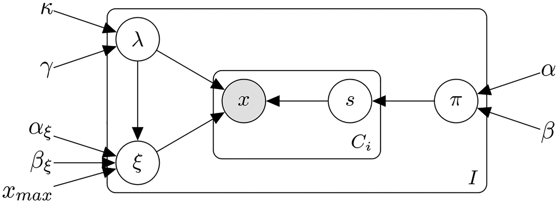
Probabilistic graphical model of the hierarchical Generalized Poisson model with a latent skipped cycle s variable to accommodate self-tracking artifacts.

We take advantage of the Generalized Poisson distribution (Consul and Famoye, 2006) for its specific parameterization that enables us to capture the uncertainty of the observed cycle lengths (its posterior can be under- or over- dispersed) and provide calibrated predictions.

The Generalized Poisson is a distribution that belongs to the class of Lagrangian distributions over discrete, non-negative integers, with parameters λ and ξ that are independent (Consul, 1989; Consul and Famoye, 2006). The probability density function (pdf) of a Generalized Poisson, hereby denoted as $\mathcal{G}\mathcal{P}(\cdot )$ follows

$$\mathcal{G}\mathcal{P}(x\mid \lambda ,\xi )=\{\begin{array}{ll}\lambda {(\lambda +\xi x)}^{x-1}\frac{e^{-\lambda -\xi x}}{x!},\hfill & \lambda >0,x=0,1,\cdots ,\hfill \\ 0,\hfill & \text{for }x>x_{max}\text{ if }\xi <0,\hfill \end{array}$$ (1)

where limits on λ and ξ are imposed to ensure that there are at least five classes with nonzero probability (Consul, 1989). The first two moments³ of a $\mathcal{G}\mathcal{P}(x\mid \lambda ,\xi )$ follow ${\mu }_x=\frac{\lambda }{(1-\xi )}$ and ${\sigma }_x^2=\frac{\lambda }{{(1-\xi )}^3}$, where we observe how the two independent parameters provide two degrees of freedom to fit the mean and the variance, separately. The Generalized Poisson can be over- or under-dispersed, depending on the value of ξ (when ξ = 0, we recover the Poisson distribution). For ξ < 0, the Generalized Poisson is under-dispersed (in comparison to a Poisson distribution) and it can be truncated to a maximum value x_max of x, requiring an additional normalizing factor $Z_{\mathcal{G}\mathcal{P}\left(\lambda ,\xi ,x_{max}\right)}$, see details in Section A.1 of the Appendix.

3.1. The hierarchical, generative process for observed cycle lengths

The proposed model, depicted in Figure 1, is a generative process with the following random (observed and unobserved) variables and parameters:

• The observed variables are the cycle lengths $x_{i,c_i}$, with c_i = {1, ⋯, C_i} cycle lengths for each individual i = {1, ⋯, I}. We denote with $s_{i,c_i}$ the (latent) number of skipped (not-reported) cycles, with c_i = {1, ⋯, C_i} cycle lengths for each individual i = {1, ⋯, I}.

• λ_i and ξ_i denote the Generalized Poisson parameters for each individual i = {1, ⋯, I}; π_i are the per-individual i = {1, ⋯, I} probability parameters of skipping a cycle.

• κ, γ are the population-level hyperparameters of a Gamma distribution prior over the λ_i; α_ξ, β_ξ the hyperparameters of a Beta distribution prior over the ξ_i; and α, β the hyperparameters of a Beta distribution prior over the skipping probabilities π_i.

We now summarize the generative process of the proposed probabilistic model. First, one draws individual cycle length and self-tracking probability parameters from the population level distributions: i.e., each individual’s ${\lambda }_i~p(\lambda \mid \kappa ,\gamma )=\mathcal{G}(\lambda \mid \kappa ,\gamma )$ and ${\xi }_i~\text{max}\left\{-1,\frac{-{\lambda }_i}{x_{max}}\right\}+\left(1-max\left\{-1,\frac{-{\lambda }_i}{x_{max}}\right\}\right)\mathcal{B}\left(\xi \mid {\alpha }_{\xi },{\beta }_{\xi }\right)$ parameters, and the the probability of each individual forgetting to track a period ${\pi }_i~p(\pi \mid \alpha ,\beta )=\mathcal{B}(\pi \mid \alpha ,\beta )$ (all distributional details are provided in Section A.2 of the Appendix). Given per-individual parameters λ_i, ξ_i, π_i, then the number of cycles a user forgets to track is drawn from a Truncated Geometric distribution with parameter π_i, i.e., $s_{i,c_i}~p\left(s\mid {\pi }_i\right)=\frac{{\pi }_i^s\left(1-{\pi }_i\right)}{{\sum }_{s=0}^{s_{max}}{\pi }_i^s\left(1-{\pi }_i\right)}$. Finally, the observed cycle length for each user i is drawn from a Generalized Poisson distribution, conditioned on the number of skipped cycles, i.e., $x_{i,c_i}~p\left(x\mid {\lambda }_i,{\xi }_i,s_{i,c_i}\right)=\mathcal{G}\mathcal{P}\left(x\mid \left(s_{i,c_1}+1\right){\lambda }_i,{\xi }_i\right)$.

3.2. The proposed model’s distributions of interest

There are two distributions that are critical for the purpose of this study: (i) the joint, over all individuals’ marginalized data (log)-likelihood, and (ii) each individual’s cycle length predictive posterior. As explained in the introduction, a Bayesian view of predictive modeling requires the derivation of the predictive distribution via marginalization of all the inherent (parametric) model uncertainties:

$$p(Y\mid x)={\int }_{\theta }p(Y\mid x,\theta )p(\theta \mid \mathcal{D})\text{d}\theta .$$ (2)

Here, we aim at marginalizing all the parameters of the model, based on the prior distribution assumptions described in Section 3.1. In our proposed model, the latent parameters θ contain both the unobserved per-cycle skips $s_{i,c_i}$ and the per-individual parameters λ_i, ξ_i and π_i, i.e., $\theta =\left\{s_{i,c_i},{\lambda }_i,{\xi }_i,{\pi }_i\right\}$. Similarly, and to reduce clutter, we denote with Θ all the hyperparameters of our model: Θ = {κ, γ, α_ξ, β_ξ, α, β}.

We clarify our notation here, where we denote a set of cycle length observations for a given individual i with $X_i={\left(x_{i,1},\cdots ,x_{i,C_i}\right)}^{\top }\in {ℝ}^{C_i}$, and the set of cycle length observations for all individuals i = {1, ⋯, I} in the population are denoted with $X={\left(X_1^{\top },\cdots ,X_I^{\top }\right)}^{\top }\in {ℝ}^{I\times C_I}$, where C_I = maxC_i, ∀i. Similarly, the set of latent skipped cycle variables for a given individual i is denoted with $S_i={\left(s_{i,1},\cdots ,s_{i,C_i}\right)}^{\top }\in {ℝ}^{C_i}$, and the set of all latent skipped cycle variables for all individuals i = {1, ⋯, I} in the population are denoted with $S={\left(S_1^{\top },\cdots ,S_I^{\top }\right)}^{\top }\in {ℝ}^{I\times C_I}$, where C_I = maxC_i, ∀i.

3.2.1. Marginalized joint data likelihood

The population level data likelihood, with marginalized parameters, can not be derived in closed form. Instead, we resort to a hybrid approach, where we analytically marginalize per-individual skipped cycles $s_{i,c_i}$ and use Monte Carlo to marginalize the per-individual parameters λ_i, ξ_i and π_i. The resulting marginalized joint data likelihood follows

$$p(X\mid \Theta )=\prod _{i=1}^I\prod _{c_i=1}^{C_i}p\left(x_{i,c_i}\mid \Theta \right)\approx \prod _{i=1}^I\frac{1}{M}\sum _{m=0}^{M}p\left(X_i\mid {\lambda }_i^{(m)},{\xi }_i^{(m)},{\pi }_i^{(m)}\right),$$ (3)

where the per-user joint likelihood is marginalized over the skipped cycles $s_{i,c_i}$, i.e.,

$$p\left(X_i\mid {\lambda }_i^{(m)},{\xi }_i^{(m)},{\pi }_i^{(m)}\right)=\prod _{c_i=1}^{C_i}\sum _{s_{i,c_i}=0}^{s_{max}}p\left(x_{i,c_i}\mid s_{i,c_i},{\lambda }_i^{(m)},{\xi }_i^{(m)}\right)p\left(s_{i,c_i}\mid {\pi }_i^{(m)}\right),$$ (4)

and evaluated with Monte Carlo parameters ${\lambda }_i^{(m)}~p(\lambda \mid \kappa ,\gamma )$, ${\xi }_i^{(m)}~p\left(\xi \mid {\lambda }_i^{(m)},{\alpha }_{\xi },{\beta }_{\xi }\right)$, and ${\pi }_i^{(m)}~p(\pi \mid \alpha ,\beta )$ drawn from their respective prior/posterior distributions (corresponding Equations (11), (12), and (13) are provided in Section A.2 of the Appendix).

The joint data likelihood is key for our training procedure, and determines the computational complexity of the fitting procedure. Given a dataset of C_i cycle lengths for i = {1, ⋯, I} users, we perform hyperparameter inference via type-II maximum likelihood estimation; that is, we find the hyperparameters $\widehat{\Theta }$ that maximize the data log-likelihood as provided in Equation (3), i.e., $\widehat{\Theta }={\text{argmax}}_{\Theta }[\text{ln}(p(X\mid \Theta ))]$.

After the training procedure, the hyperparameters Θ = {κ, γ, α_ξ, β_ξ, α, β} used for drawing the Monte Carlo parameters in Equation (3) will be replaced with the learned population level hyperparameters $\widehat{\Theta }$.

We note that the hierarchical nature of the proposed model enables distributed learning, with not only computational, but also privacy benefits: mHealth users do not need to share their data (they can locally compute their individualized predictions), and only need to share per-user data log-likelihood estimates for population-level hyperparameter inference (see Section A.6 of the Appendix for a more detailed discussion).

3.2.2. Cycle length predictive posterior

We derive the marginalized predictive posterior of the next cycle length $x_{i,c_{new}}$ after observing per-user cycle lengths X_i,

$$p\left(x_{i,c_{new}}\mid X_i,\Theta \right)=\frac{{\int }_{{\lambda }_i}{\int }_{{\xi }_i}{\int }_{{\pi }_i}p\left(x_{i,c_{new}}\mid {\lambda }_i,{\xi }_i,{\pi }_i\right)p\left(X_i\mid {\lambda }_i,{\xi }_i,{\pi }_i\right)p\left({\lambda }_i,{\xi }_i,{\pi }_i\mid \Theta \right)\text{d}{\lambda }_i\text{d}{\xi }_i\text{d}{\pi }_i}{{\int }_{{\lambda }_i}{\int }_{{\xi }_i}{\int }_{{\pi }_i}p\left(X_i\mid {\lambda }_i,{\xi }_i,{\pi }_i\right)p\left({\lambda }_i,{\xi }_i,{\pi }_i\mid \Theta \right)\text{d}{\lambda }_i\text{d}{\xi }_i\text{d}{\pi }_i},$$ (5)

for which we need to compute p(X_i|λ_i, ξ_i, π_i) as in Equation (4). We again marginalize per-individual skipped cycles $s_{i,c_{new}}$ in

$$p\left(x_{i,c_{new}}\mid {\lambda }_i,{\xi }_i,{\pi }_i\right)=\sum _{s_{i,c_{new}}=0}^{s_{max}}p\left(x_{i,c_{new}}\mid s_{i,c_{new}},{\lambda }_i,{\xi }_i\right)p\left(s_{i,c_{new}}\mid {\pi }_i\right).$$ (6)

One can readily compute the above via Monte Carlo, by drawing from the parameter posterior p(λ_i, ξ_i, π_i|X_i, Θ) as described in Equation (17) in Section A.3 of the Appendix, or via Importance Sampling by drawing from the prior p(λ_i, ξ_i, π_i|Θ) and weighting samples with p(X_i|λ_i, ξ_i, π_i) as in Equation (4). After the training procedure, the hyperparameters Θ above will be replaced with the learned population level hyperparameters $\widehat{\Theta }$.

In addition, we note that the above cycle length predictive posterior, as well as the skipping probability predictive posterior, can be updated as subsequent days of the next cycle pass by, which we have derived in Sections A.4 and A.5 of the Appendix, respectively.

4. Cohort

Real-world Menstrual mHealth Dataset⁴.

We leverage a de-identified self-tracked dataset from Clue by BioWink (Clue, 2021), comprised of 117, 014, 597 self-tracking events over 378, 694 users. Clue app users input overall personal information at sign-up, such as age and birth control type. The dataset contains information from 2015–2018 for users worldwide, covering countries within North and South America, Europe, Asia and Africa. In the entire dataset, the median number of tracked menstrual cycles is 11. Inclusion criteria into the cohort were: (1) users likely to have ovulatory cycles, that is aged 21–33 with natural cycle (i.e., no contraception); (2) users with at least 11 cycles tracked. The cohort resulted in 186, 106 menstruators. For the experiments described in this paper, we randomly select a subset of 50, 000 users. The summary statistics of the overall and the selected cohort for the experiments are provided in Table 1. We observe minimal differences in cycle length and period length statistics between the full cohort and the selected cohort.

Table 1:

Summary statistics for the overall cohort and the 50, 000 random user subset. Note that race/ethnicity information is not available from this de-identified dataset.

Summary statistic	Full cohort	Selected cohort
Total number of users	186,106	50,000
Total number of cycles	2,047,166	550,000
Cycle length in days: mean±sd (median)	30.7±7.9 (29)	30.6±7.7 (29)
Period length in days: mean±sd (median)	4.1±1.8 (4)	4.1±1.8 (4)
Age in years: mean±sd (median)	25.6±3.6 (25)	25.6±3.6 (25)

Data Extraction and Feature choices.

Even though Clue’s mHealth app users can self-track multiple symptoms over time, we focus on period data only, i.e., users’ self-reports on which days they have their period. A period is defined as sequential days of bleeding (greater than spotting and within ten days after the first greater than spotting bleeding event) unbroken by no more than one day on which only spotting or no bleeding occurred. We use cycle lengths as input to our proposed model, where we define a menstrual cycle as the span of days from the first day of a period through to and including the day before the first day of the next period (Vitzthum, 2009). We discard any cycle a user has indicated to be excluded from their history —e.g., if the user felt that the cycle was not representative of their typical menstruation due to a medical procedure or changes in birth control.

Synthetic Datasets⁵.

To assess the ability of our model to recover ground truth (only possible with simulated data), we leverage two alternative generative processes. A Poisson generative model of cycle lengths, where the observed cycle lengths are drawn from the generative model by Li et al. (2021); i.e., cycle length data follows a Poisson distribution (see model and parameterization details in Appendix B.1). A Generalized Poisson generative model of cycle lengths, where the observed data are drawn from the generative model as proposed in Section 3; i.e., cycle length data is drawn from a Generalized Poisson distribution (full details are provided in Appendix B.2). For each of the simulated scenarios, we draw cycle length data for 50, 000 users, with C_i = 11 cycles for each user.

5. Evaluation

5.1. Evaluation Approach: Real and Synthetic Study Designs

Our objective is to accurately predict the next cycle length of a mHealth menstrual app user, based on their previously-tracked cycle lengths. To that end, we train the proposed generative model (as described in Section 3) and several baselines (described in Section 5.1.1) on the cycle length information from each of the datasets described in Section 4.

We train on the first 10 cycle lengths of each user (C_i = 10, ∀i) and, given the hyperparameters $\widehat{\Theta }$ learned via the training procedure, we predict the next cycle length (i.e., each user’s 11th cycle) via the predictive posterior in Section 3.2.2. Consequently, the train-test split is within, and not across, individuals: we train personalized models with each individual’s first 10 cycles, and evaluate our individualized predictions with respect to each user’s next cycle length.

We average our results (and provide standard deviations) over k = 5 realizations to aggregate over the inherent uncertainties of the training and testing procedure: e.g., robustness to random number generator seeds, Monte Carlo sampling and the optimization procedure.

We note that the learned predictive posterior $p\left(x_{i,c_{new}}=x\mid X_i,\widehat{\Theta }\right)$ provides per-user fully probabilistic predictions, i.e., it computes the probability of the next cycle length $x_{i,c_{new}}$ being of length $x\in \mathbb{N}$ for each user i. Therefore, we are enabled to provide both point estimate predictions (e.g., the mean or mode of the predictive distribution), as well as to evaluate how well-calibrated the predicted cycle length posterior is.

5.1.1. Baselines

We compare the performance of our model to the following baselines⁶:

• CNN: a 2-layer convolutional neural network with a 3-dimensional kernel.

• RNN: a 2-layer bidirectional recurrent neural network with a 3-dimensional hidden state.

• LSTM: a 2-layer Long Short-Term Memory neural network with a 3-dimensional hidden state.

• Poisson model: the Poisson-based predictive model proposed by Li et al. (2021).

5.1.2. Prediction Metrics

We use several accuracy metrics for the evaluation of next cycle length point estimates $\widehat{x_{i,c_{new}}}$ with respect to true cycle lengths $x_{i,c_{new}}$ for all I users in the cohort. The root-mean squared error, $\text{RMSE}=\sqrt{\frac{{\sum }_{i=1}^I{\left(x_{i,c_{new}-\widehat{x_{i,c_{new}}}}\right)}^2}{I}}$; the median squared error, $\text{MedianSE}=\mathcal{M}\mathit{\text{edian}}\left[{\left(x_{i,c_{new}}-\widehat{x_{i,c_{new}}}\right)}^2\right]$ (which is less sensitive to outliers than the RMSE); the mean absolute error, $\text{MAE}=\frac{{\sum }_{i=1}^I\left|x_{i,c_{new}}-\widehat{x_{i,c_{new}}}\right|}{I}$; and the median absolute error, $\text{MedianSE}=\mathcal{M}\mathit{\text{edian}}\left[\left|x_{i,c_{new}}-\widehat{x_{i,c_{new}}}\right|\right]$.

5.1.3. Calibration Metrics

We leverage a diverse set of calibration metrics and scoring rules, both visual and numeric, to evaluate the uncertainty quantification of the generative models’ predictive posteriors. On one hand, we consider the following, most often visually presented, calibration metrics:

The probability integral transform (PIT), defined as the value that the cumulative density function (CDF) of a predictive model F(·) attains at the observation, i.e., p_i = F(x_i), where x_i ~ g(·) is drawn from the true (yet unknown) generating mechanism, with CDF G(·). For continuous true G(·) and predictive F(·), p_i has a uniform distribution if the predictions are ideal, i.e., if F(·) = G(·). PITs are most often reported as a histogram over the set of observed instances x_i, ∀i; and for the ideal case, the histogram of the PIT values is (asymptotically) uniform. The uniformity of the PIT is a necessary, but not sufficient, condition for the predictive distribution to be ideal —Gneiting et al. (2007) provides a detailed explanation of PIT’s limitations. Visual assessment of PIT histograms provides insights into the calibration deficiencies of a predictive posterior: hump-shaped histograms indicate over-dispersion (i.e., prediction intervals are too wide), while U-shaped histograms correspond to under-dispersion (i.e., too narrow predictive distributions). Note that triangle-shaped histograms indicate biased predictive distributions. Since its proposal by Rosenblatt (1952), many authors have extended and studied PIT’s advantages and disadvantages —see Section 3 in (Gneiting et al., 2007).

The marginal calibration plot (MCP), defined as the difference between the predictive CDF F(·) and the empirical CDF of the observed data $\widehat{G}(\cdot )$ (Gneiting et al., 2007), i.e., $F\left(x_i\right)-\widehat{G}\left(x_i\right),\forall x_i$. The most straightforward approach is to visualize the above difference over all observed instances, towards assessing the marginal calibration of the predictive distribution. The marginal calibration is concerned with the closeness between the predictive outcomes (i.e., predictive distribution) and the actual, observed outcomes (i.e., the data). The interested reader can find in Gneiting et al. (2007) a rigorous study of how, under mild regularity conditions, marginal calibration is a necessary and sufficient condition for the asymptotic equality between the average predictive CDF and the empirical CDF of the observations. Visually, one expects minor fluctuations under the hypothesis of marginal calibration (i.e., the MCP is almost flat), while major excursions from the origin indicate a lack of marginal calibration.

On the other hand, to quantify with a single numerical score how closely a model’s predictive distribution matches each user’s observed cycle lengths, we consider several scoring rules. The selected scores presented below form a comprehensive set of summary measures of predictive performance, as they address calibration and sharpness simultaneously (Gneiting et al., 2007). We note that all these are proper scoring rules⁷ in general, and strictly proper⁸ under quite general conditions —a detailed, theoretically grounded review of the above and other scoring rules is provided in (Gneiting and Raftery, 2007). We define them here for predictive distributions on the natural line $x\in \mathbb{N}$, but they are scoring rules that can readily accommodate continuous variables.

The quadratic or Brier score, defined as $\text{BrierS}\left(p,x_i\right)=-\sum _{x=1}^{x_{max}}{\left(\delta \left(x-x_i\right)-p(x)\right)}^2$.

The pseudo-spherical score, defined as $\text{PseudoS}\left(p,x_i\right)=\frac{p{\left(x_i\right)}^{\alpha -1}}{{\Vert p\Vert }_{\alpha }^{\alpha -1}}$, which reduces to the more common Spherical score when α = 2, used in our results.

The logarithmic score, defined as the log-likelihood of the observation x_i under the predicted posterior p(·): LogS(p, x_i) = logp(x_i), which relates directly to the negative Shannon entropy and the commonly used log-likelihood metric. Interestingly, this score emerges as a limiting case of the pseudospherical score with α → 1 when it is suitably scaled.

The continuous ranked probability score (CRPS), defined in terms of the CDF F(·) of the predictive posterior, i.e., $\text{CRPS}\left(F,x_i\right)=-{\int }_{-\infty }^{\infty }{\left(F(x)-\mathbb{1}\left[x_i\right]\right)}^2\text{d}x$, and corresponds to the integral of the Brier scores for the associated binary probability forecasts at all realvalued thresholds —note that when dealing with integers in the natural line, the thresholds are countable, resulting in a sum over a finite number of bins. The motivation for the CRPS is to overcome several limitations regarding other metrics on continuous variables. If Lebesgue densities on the real line are used to predict discrete observations, then the logarithmic score encourages the placement of artificially high density ordinates on the target values, and no credit is given for assigning high probabilities to values near but not identical to the one materializing. As such, defining scoring rules in terms of predictive CDFs (instead of probability density functions) has bee argued for by Gneiting et al. (2007).

5.2. Validation on the synthetic cycle length dataset

We first showcase the added flexibility of our proposed method by leveraging the synthetic datasets described in Section 4. Our synthetic data results (presented in Section B) demonstrate that the proposed model provides better uncertainty quantification capabilities than the alternative proposed by Li et al. (2021), both in terms of predictive accuracy and calibration metrics. Specifically, when the cycle length data is Poisson distributed, both models can accurately fit the data and provide well-calibrated predictions: all scoring rules are identical for both models, see Section B.1.

On the contrary, when the observed cycle length data is drawn from a Generalized Poisson that is under-dispersed, we observe that the Proposed model clearly outperforms the Poisson model both in terms of predictive accuracy and calibration metrics. Specifically, we note (see Figures in Section B.2) that the PIT of the Poisson model is hump-shaped, i.e., it is clearly over-dispersed, while the Proposed model’s PIT histogram is close to a uniform distribution. In addition, the MCP plot for the Proposed model hardly deviates from the origin, while the Poisson model showcases a calibration mismatch around $x_{c_{new}}=20$. Overall, these results validate that a Generalized Poisson based model is able to more flexibly adjust to the uncertainty of observed cycle lengths and provide well-calibrated predictions.

5.3. Results on the real-world mHealth dataset

We now present results for all the considered models (generative and neural network based, as described in Section 5.1.1) in the real-world cycle length dataset presented in Section 4. We provide in Table 2 point estimate results for all the models at the next day of the last observed cycle length (i.e., day 0 of the next cycle), as per the metrics in Section 5.1.2.

Table 2:

Real-world dataset: Point estimate results for all models

Model	RMSE	MedianSE	MAE	MedianAE
CNN	7.243 (± 0.000)	11.089 (± 0.341)	4.379 (± 0.016)	3.330 (± 0.051)
LSTM	6.730 (± 0.017)	4.303 (± 0.515)	3.626 (± 0.082)	2.071 (± 0.123)
RNN	6.820 (± 0.062)	5.606 (± 0.783)	3.846 (± 0.071)	2.362 (± 0.166)
Poisson model (mode)	6.856 (± 0.023)	4.000 (± 0.000)	3.451 (± 0.006)	2.000 (± 0.000)
Proposed model (mode)	6.790 (± 0.007)	4.000 (± 0.000)	3.459 (± 0.003)	2.000 (± 0.000)
Poisson model (mean)	6.690 (± 0.002)	4.818 (± 0.292)	3.639 (± 0.042)	2.194 (± 0.066)
Proposed model (mean)	6.691 (± 0.005)	4.237 (± 0.064)	3.592 (± 0.009)	2.058 (± 0.015)

First, we conclude that in our use case, black-box neural network architectures do not provide any prediction accuracy advantage, which aligns with results presented by Li et al. (2021). Results showcasing the calibration shortcomings of the studied neural network architectures are presented in Appendix B.3. Second, we notice that our model’s predictive accuracy is as good as the Poisson-based alternative of Li et al. (2021) when the mode of each model’s predictive posterior is used as the predicted cycle length point estimate.

Third, as both the Poisson model and our Proposed model provide a full predictive posterior density over the set of natural integers $x_{i,c_{new}}\in \mathbb{N}$, we compare their performance when considering the mean and the mode of the predictive posterior as point estimates. We observe a slightly better performance of our Proposed model, both in cohort-level average results as well as in their variability, specially so for the metrics most robust to outliers (i.e., MedianSE, MAE and MedianAE). This performance difference suggests that the mean and the mode do not coincide in each model’s predictive distributions, which we hypothesize is explained by the dispersion of such densities, i.e., the shape and width of their posterior densities around the mode.

To elucidate the added flexibility of the Proposed model to capture cycle length uncertainty, we first visualize in Figure 2 the scatter plot of per-user true cycle length average (x-axis) versus each model’s per-user expected cycle length (y-axis). Each dot in Figure 2 represents a user, colored by the cycle length variability of each user: i.e., lighter color for users with low cycle length variability, darker color for users with high cycle length variability.

Figure 2:

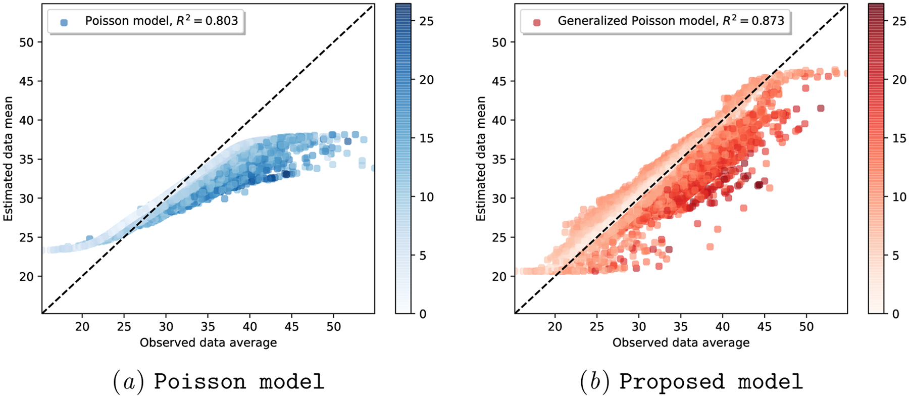
Real-world dataset: Fitting sufficient statistics of observed cycle length data, colored by user cycle length variability. The colorbar indicates the standard deviation of observed per-user cycle lengths.

We observe that the Poisson model struggles to find the right mean-variance balance: note how skewed the scatter plot in Figure 2(a)subfigure is, with most of the users (irrespective of their variability) situated below and to the right side of the x = y line.

We hypothesize that this skewness is due to the rigid parameterization of a Poisson distribution: there is only one degree of freedom (i.e., λ_i) that determines both the mean and the variance of each user’s cycle lengths. On the contrary, the two-parameter Generalized Poisson can adjust, via λ_i and ξ_i, both the mean and the variance of per-user cycle lengths. As shown in Figure 2(b)subfigure, this ability to quantify the data uncertainty allows the Proposed model to fit the data better (R² = 0.873) than the Poisson model (R² = 0.803).

We now turn our attention to the full posterior predictive distribution of each of the models, to investigate their uncertainty quantification capabilities.

In Figure 3, we illustrate the cycle length predictive posterior of each generative model for a randomly selected user, as days of the subsequent cycle proceed (the form of this per-day cycle length posterior is described in Section A.4 of the Appendix). Note how the Proposed model consistently provides less uncertain (i.e., under-dispersed) predictions.

Figure 3:

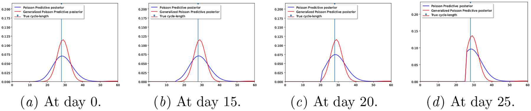
Real-world dataset: Predictive posteriors for a random user at different days of the next cycle.

We showcase in Table 3 that the under-dispersed predictive posterior of the Proposed model occurs for all users in the dataset, by providing the average posterior predictive width at level α. The values provided in the table indicate the width (in days) of the (1-α) centered probability mass, i.e., the width of the posterior predictive distribution between quantiles α/2 and 1 − α/2, as illustrated in Figure 4, for the Proposed model’s posterior of Figure 3 with α = 0.5 at day 0. Note that the posterior predictive width in Table 3 for the 20% posterior mass of our Proposed model is less that 2 days, while it’s almost 3 for the Poisson model. Besides, the 50% posterior mass width of the Poisson model is almost 8 days (i.e., the next period is predicted to occur within an interval longer than a week), raising the question on how useful such prediction is for mHealth users.

Table 3:

Real-world dataset: Posterior predictive width at day 0 of next cycle.

Model	Posterior predictive interval width at level α.
	α = 0.8	α = 0.5	α = 0.2
Poisson model	2.925 (± 0.005)	7.835 (± 0.026)	15.248 (± 0.074)
Proposed model	1.846 (± 0.014)	4.940 (± 0.038)	9.692 (± 0.089)

Figure 4.

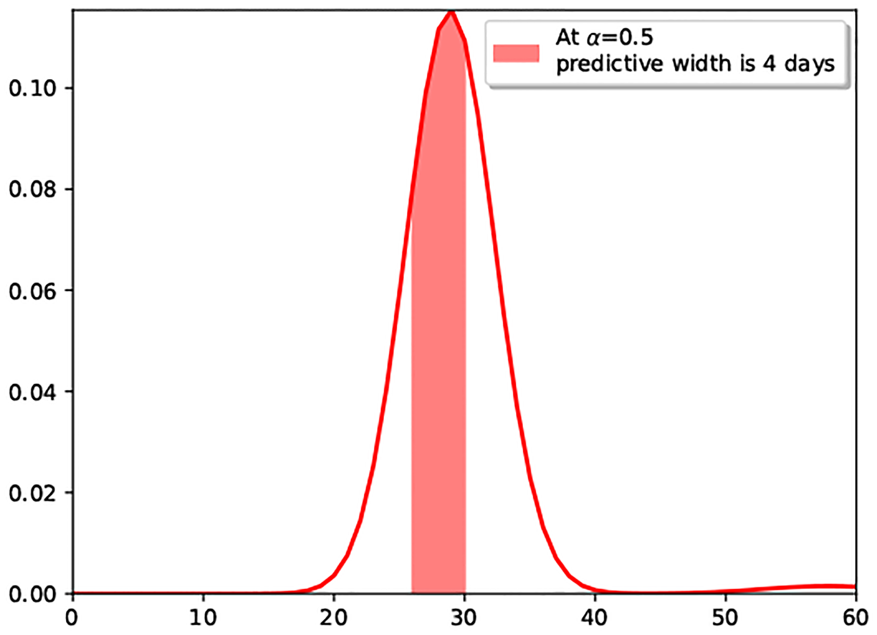
Posterior predictive width at day 0.

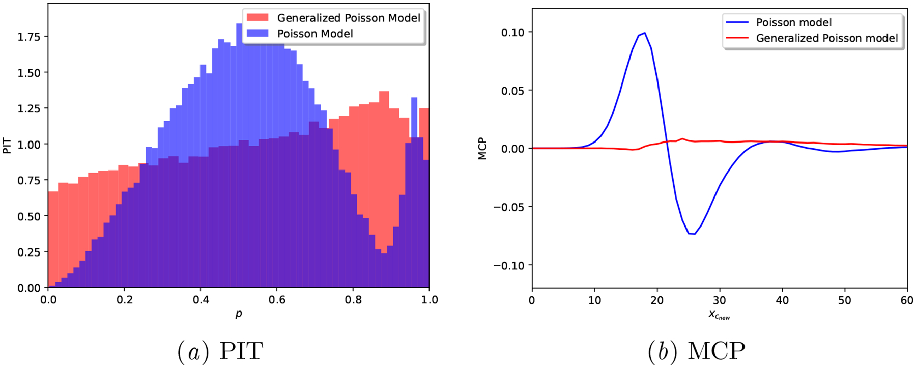
In order to settle our claim that the Generalized Poisson based model provides better calibrated predictions, we provide in Table 4 the average results for all the considered scoring rules described in Section 5.1.3, along with PIT and MCP plots in Figure 5: note how over-dispersed (hump-shaped) the Poisson model is in Figure 5(a)subfigure, and how, in Figure 5(b)subfigure, we observe a lack of posterior sharpness for the Poisson model. The calibration shortcomings of neural network based models are showcased in Appendix B.3.

Table 4:

Real-world dataset: Calibration results for the generative models, higher is better.

Model	Brier score	Spherical score	Logarithmic score	CRPS
Poisson model	−0.931 (± 0.000)	0.266 (± 0.000)	−3.022 (± 0.001)	−2.922 (± 0.003)
Proposed model	−0.910 (± 0.000)	0.299 (± 0.000)	−2.855 (± 0.002)	−2.740 (± 0.001)

Figure 5:

Real-world dataset: Calibration plots for a realization of each generative model.

As demonstrated across the variety of considered metrics, we can conclude that the Proposed model provides better calibrated results. However, as shown in Figure 5, the Proposed model is still not ideal: it does not result in a fully uniform PIT and its MCP slightly fluctuates away from 0 around the median cycle length (29 days) of the cohort.

To conclude, we emphasize that the Proposed model provides under-dispersed (i.e., less uncertain) and better calibrated cycle length predictions than the state-of-the-art alternative of Li et al. (2021), both as demonstrated at the user and population level. In addition, we showcase in Figure 6 how the under-dispersed predictive posterior of our Proposed model provides additional (across population and point estimate-based) predictive benefits: the predictive accuracy of the Proposed model is better than that of the Poisson model as days of the next cycle proceed. This is especially evident about a week before the median cycle length of the studied cohort. In other words, the Proposed model outperforms other models’ predictive accuracy 6 to 8 days before the next cycle length starts.

Figure 6.

Real-world dataset: Prediction accuracy at different days of the next cycle

6. Discussion

We proposed a flexible generative model that provides accurate, well-calibrated predictions of menstrual cycle lengths based on self-tracked mobile health data. Specifically, we investigated how to overcome certain limitations of a Poisson regression-based cycle length model by making use of a more flexible distribution, namely the Generalized Poisson. Our proposed model allows for accurate uncertainty quantification: it provides two degrees of freedom to fit the mean and variance of the observed cycle lengths. The model’s ξ parameter allows for controlling the dispersion of its predictive posterior, which enables better calibrated predictive posteriors, as demonstrated by our results.

Due to the well-calibrated predictions, the model not only yields improved predictive accuracy as the cycle days proceed (see Figure 6), but provides more meaningful (i.e., less uncertain) cycle length predictions (see Figure 3).

We argue that more certain cycle length predictions, like the ones provided by our proposed model, may benefit mHealth users: they help increase trust in the model and may mitigate user notification fatigue, a well-known phenomenon where users ignore prediction notifications if they occur too often and with low sensitivity.

More broadly, we argue that uncertainty quantification and calibration are critical in the domain of health and healthcare. One must account for the variability of the studied physiology, and adjust to the uncertainties of the data collection and reporting process. To that end, we have presented a diverse tool-set of calibration metrics that are of use in assessing the predictions of our proposed model, and argue that they should be readily incorporated into the practice of machine learning in healthcare.

We acknowledge several limitations of our work: (i) while we argue that less uncertain cycle length predictions may reduce mHealth user notification fatigue, we leave to future work to validate such a hypothesis; and (ii) our model includes features of the menstrual cycle only related to its length. While it is a minimal feature that we know will be present across many app users, there might be additional features like signs and symptoms of the menstrual cycle that may improve our predictive model.

Overall, our work showcases that generative models can accommodate the idiosyncrasies of mHealth data to provide well-calibrated, accurate predictions. Less uncertain cycle length predictions are beneficial for menstrual health researchers, mHealth users and developers.

Appendix A. Methods

A.1. The Generalized Poisson

The Generalized Poisson is a distribution that belongs to the class of Lagrangian distributions over discrete, non-negative integers, with parameters λ and ξ that are independent (Consul, 1989; Consul and Famoye, 2006).

The probability density function (pdf) of a Generalized Poisson, hereby denoted as $\mathcal{G}\mathcal{P}(\cdot )$, follows

$$\mathcal{G}\mathcal{P}(x\mid \lambda ,\xi )=\{\begin{array}{ll}\lambda {(\lambda +\xi x)}^{x-1}\frac{e^{-\lambda -\xi x}}{x!},\hfill & \lambda >0,x=0,1,\cdots ,\hfill \\ 0,\hfill & \text{for }x>x_{max}\text{ if }\xi <0,\hfill \end{array}$$ (7)

where limits on λ and ξ are imposed to ensure that there are at least five classes with nonzero probability (Consul, 1989).

The first two moments of a $\mathcal{G}\mathcal{P}(x\mid \lambda ,\xi )$ follow

$${\mu }_x=\frac{\lambda }{(1-\xi )},$$ (8a)

$${\sigma }_x^2=\frac{\lambda }{{(1-\xi )}^3},$$ (8b)

and other moments of interest can be computed in closed form, see (Consul and Famoye, 2006) for a full characterization of this distribution.

The Generalized Poisson can be over- or under-dispersed, depending on the value of ξ: when ξ = 0, we recover the Poisson distribution. Specifically, for ξ < 0, the Generalized Poisson is under-dispersed (in comparison to a Poisson distribution) and it can be truncated to a maximum value x_max of x, requiring an additional normalizing factor $Z_{\mathcal{G}\mathcal{P}\left(\lambda ,\xi ,x_{max}\right)}$:

$$x~\mathcal{G}\mathcal{P}(x\mid \lambda ,\xi )=\{\begin{array}{ll}\frac{\lambda {(\lambda +\xi x)}^{x-1}\frac{e^{-\lambda -\xi x}}{x!}}{Z_{\mathcal{G}\mathcal{P}\left(\lambda ,\xi ,x_{max}\right)}},\hfill & x=0,1,\cdots ,\hfill \\ 0,\hfill & \text{for }x>x_{max}\text{ if }\xi <0,\hfill \end{array}$$ (9)

with

$$Z_{\mathcal{G}\mathcal{P}\left(\lambda ,\xi ,x_{max}\right)}=\sum _{x=0}^{x_{max}}\lambda {(\lambda +\xi x)}^{x-1}\frac{e^{-\lambda -\xi x}}{x!}.$$ (10)

A.2. The hierarchical, generative process for observed cycle lengths

The proposed model, depicted in Figure 1, is a generative process with the following random (observed and unobserved) variables and parameters:

• The observed variables are the cycle lengths $x_{i,c_i}$, with c_i = {1, ⋯, C_i} cycle lengths for each individual i = {1, ⋯, I}.

• We denote with $s_{i,c_i}$ the (latent) number of skipped (not-reported) cycles, with c_i = {1, ⋯, C_i} cycle lengths for each individual i = {1,··· ,I}.

• λ_i and ξ_i denote the Generalized Poisson parameters for each individual i = {1, ⋯, I}.

• π_i are the parameters defining the per-individual i = {1, ⋯, I} probability of skipping a cycle.

• κ, γ are the population-level hyperparameters of a Gamma distribution prior over the λ_i.

• α_ξ, β_ξ are the population-level hyperparameters of a Beta distribution prior over the ξ_i.

• α, β are the population-level hyperparameters of a Beta distribution prior over the skipping probabilities π_i.

We now describe in detail the generative process of the proposed probabilistic model. First, one draws individual cycle length and self-tracking probability parameters from the population level distributions:

1. The parameter λ_i of each individual’s Generalized Poisson is drawn from a population-level Gamma distribution with hyperparameters κ and γ

   $${\lambda }_i~p(\lambda \mid \kappa ,\gamma )=\mathcal{G}(\lambda \mid \kappa ,\gamma )=\frac{{\gamma }^{\kappa }}{\Gamma (\kappa )}{\lambda }^{\kappa -1}{e}^{-\gamma \lambda },\text{ for }\lambda >0\text{ and }\kappa ,\gamma >0.$$ (11)
2. The parameter ξ_i of each individual’s Generalized Poisson is drawn, conditioned on each λ_i, from a shifted and scaled population-level Beta distribution with hyperparameters α_ξ and β_ξ, so that ${\xi }_i\in \left[\text{max}\left\{-1,\frac{-{\lambda }_i}{x_{max}}\right\},1\right]$:

   $${\xi }_i~\text{max}\left\{-1,\frac{-{\lambda }_i}{x_{max}}\right\}+\left(1-\text{max}\left\{-1,\frac{-{\lambda }_i}{x_{max}}\right\}\right)\mathcal{B}\left(\xi \mid {\alpha }_{\xi },{\beta }_{\xi }\right),\text{ for }\xi \in [0,1],$$ (12)

   where $\mathcal{B}\left(\xi \mid {\alpha }_{\xi },{\beta }_{\xi }\right)=\frac{\Gamma \left({\alpha }_{\xi }+{\beta }_{\xi }\right)}{\Gamma \left({\alpha }_{\xi }\right)\Gamma \left({\beta }_{\xi }\right)}{\xi }^{{\alpha }_{\xi }-1}{(1-\xi )}^{{\beta }_{\xi }-1}$ for ξ ∈ [0, 1] and α_ξ, β_ξ > 0.
3. The probability π_i of each individual forgetting to track a period is drawn from a population-level Beta distribution with hyperparameters α and β,

   $${\pi }_i~p(\pi \mid \alpha ,\beta )=\mathcal{B}(\pi \mid \alpha ,\beta )=\frac{\Gamma (\alpha +\beta )}{\Gamma (\alpha )\Gamma (\beta )}{\pi }^{\alpha -1}{(1-\pi )}^{\beta -1},\text{ for }\pi \in [0,1]\text{ and }\alpha ,\beta >0.$$ (13)

   Given per-individual parameters λ_i, ξ_i, π_i, then:
4. The number of cycles a user forgets to track $s_{i,c_i}$ is drawn from a Truncated Geometric distribution with parameter π_i, i.e.,

   $$s_{i,c_i}~p\left(s\mid {\pi }_i\right)=\frac{{\pi }_i^s\left(1-{\pi }_i\right)}{{\sum }_{s=0}^{s_{max}}{\pi }_i^s\left(1-{\pi }_i\right)}=\frac{{\pi }_i^s}{{\sum }_{s=0}^{s_{max}}{\pi }_i^s}=\frac{{\pi }_i^s\left(1-{\pi }_i\right)}{\left(1-{\pi }_i^{\left(s_{max}+1\right)}\right)},\text{ for }s\in \mathbb{N}$$ (14)
5. Each true (unobserved) cycle length x is drawn from a Generalized Poisson distribution parameterized with per-individual λ_i and ξ_i, i.e.,

   $$x~p\left(x\mid {\lambda }_i,{\xi }_i\right)=\mathcal{G}\mathcal{P}\left(x\mid {\lambda }_i,{\xi }_i\right)=\{\begin{array}{ll}{\lambda }_i{\left({\lambda }_i+{\xi }_{i}x\right)}^{x-1}\frac{e^{-{\lambda }_i-{\xi }_{i}x}}{x!},\hfill & x=0,1,\cdots ,\hfill \\ 0,\hfill & \text{for }x>x_{max}\text{ if }{\xi }_i<0.\hfill \end{array}$$ (15)
6. Finally, the observed cycle length $x_{i,c_i}$ for user i is drawn from a Generalized Poisson distribution, conditioned on the number of skipped cycles $s_{i,c_i}$, i.e.,

   $$x_{i,c_i}~p\left(x\mid s_{i,c_i},{\lambda }_i,{\xi }_i\right)=\sum _{s=0}^{s_{i,c_i}}p\left(x\mid s,{\lambda }_i,{\xi }_i\right)=\mathcal{G}\mathcal{P}\left(x\mid \left(s_{i,c_1}+1\right){\lambda }_i,{\xi }_i\right).$$ (16)

   Note that this distribution results from the property of Generalized Poissons that the sum of two independent Generalized Poisson variables $X~\mathcal{G}\mathcal{P}\left({\lambda }_1,\xi \right)$ and $Y~\mathcal{G}\mathcal{P}\left({\lambda }_2,\xi \right)$ follows another Generalized Poisson: $X+Y~\mathcal{G}\mathcal{P}\left({\lambda }_1+{\lambda }_2,\xi \right)$, (Consul and Famoye, 2006).

A.3. The model’s posterior parameter distributions

In a similar approach to the joint data likelihood, we can analytically marginalize the skipped cycles and compute a MC approximation to each parameter posterior, as described below:

$$p\left({\lambda }_i,{\xi }_i,{\pi }_i\mid X_i,\Theta \right)=\frac{p\left(X_i,{\lambda }_i,{\xi }_i,{\pi }_i\mid \Theta \right)}{p\left(X_i\mid \Theta \right)}=\frac{p\left(X_i,{\lambda }_i,{\xi }_i,{\pi }_i\mid \Theta \right)}{{\int }_{{\lambda }_i}{\int }_{{\xi }_i}{\int }_{{\pi }_i}p\left(X_i,{\lambda }_i,{\xi }_i,{\pi }_i\mid \Theta \right)\text{d}{\lambda }_i\text{d}{\xi }_i\text{d}{\pi }_i}$$ (17a)

$$=\frac{p\left(X_i\mid {\lambda }_i,{\xi }_i,{\pi }_i\right)p\left({\lambda }_i,{\xi }_i,{\pi }_i\mid \Theta \right)}{{\int }_{{\lambda }_i}{\int }_{{\xi }_j}{\int }_{{\pi }_i}p\left(X_i\mid {\lambda }_i,{\xi }_i,{\pi }_i\right)p\left({\lambda }_i,{\xi }_i,{\pi }_i\mid \Theta \right)\text{d}{\lambda }_i\text{d}{\xi }_i\text{d}{\pi }_i}$$ (17b)

$$=\frac{p\left(X_i\mid {\lambda }_i,{\xi }_i,{\pi }_i\right)p\left({\lambda }_i\mid \kappa ,\gamma \right)p\left({\xi }_i\mid {\lambda }_i,{\alpha }_{\xi },{\beta }_{\xi }\right)p\left({\pi }_i\mid \alpha ,\beta \right)}{{\int }_{{\lambda }_i}{\int }_{{\xi }_i}{\int }_{{\pi }_i}p\left(X_i\mid {\lambda }_i,{\xi }_i,{\pi }_i\right)p\left({\lambda }_i\mid \kappa ,\gamma \right)p\left({\xi }_i\mid {\lambda }_i,{\alpha }_{\xi },{\beta }_{\xi }\right)p\left({\pi }_i\mid \alpha ,\beta \right)\text{d}{\lambda }_i\text{d}{\xi }_i\text{d}{\pi }_i}$$ (17c)

$$\approx \sum _{m_{\lambda }=1}^{M_{\lambda }}\sum _{m_{\xi }=1}^{M_{\xi }}\sum _{m_{\pi }=1}^{M_{\pi }}\frac{p\left(X_i\mid {\lambda }_i^{\left(m_{\lambda }\right)},{\xi }_i^{\left(m_{\xi }\right)},{\pi }_i^{\left(m_{\pi }\right)}\right)}{{\sum }_{m_{\lambda }=1}^{M_{\lambda }}{\sum }_{m_{\xi }=1}^{M_{\xi }}{\sum }_{m_{\pi }=1}^{M_{\pi }}p\left(X_i\mid {\lambda }_i^{\left(m_{\lambda }\right)},{\xi }_i^{\left(m_{\xi }\right)},{\pi }_i^{\left(m_{\pi }\right)}\right)},$$ (17d)

$$\text{with }p\left(X_i\mid {\lambda }_i^{\left(m_{\lambda }\right)},{\xi }_i^{\left(m_{\xi }\right)},{\pi }_i^{\left(m_{\pi }\right)}\right)=\prod _{c_i=1}^{C_i}p\left(x_{i,c_i}\mid {\lambda }_i^{(m)},{\xi }_i^{(m)},{\pi }_i^{(m)}\right)$$ (17e)

$$=\prod _{c_i=1}^{C_i}\sum _{s_{i,c_i}=0}^{s_{max}}p\left(x_{i,c_i}\mid s_{i,c_i},{\lambda }_i^{(m)},{\xi }_i^{(m)}\right)p\left(s_{i,c_i}\mid {\pi }_i^{(m)}\right),$$ (17f)

$$\text{and }\{\begin{array}{l}{\lambda }_i^{\left(m_{\lambda }\right)}~p\left({\lambda }_i\mid \kappa ,\gamma \right),m_{\lambda }=1,\cdots ,M_{\lambda },\hfill \\ {\xi }_i^{\left(m_{\xi }\right)}~p\left({\xi }_i\mid {\lambda }_i^{\left(m_{\lambda }\right)}{\alpha }_{\xi },{\beta }_{\xi }\right),m_{\xi }=1,\cdots ,M_{\pi },\hfill \\ {\pi }_i^{\left(m_{\pi }\right)}~p\left({\pi }_i\mid {\alpha }_{\pi },{\beta }_{\pi }\right),m_{\pi }=1,\cdots ,M_{\pi }.\hfill \end{array}$$ (17g)

A.4. The model’s predictive cycle length posterior by day

Our model allows for updating next cycle length predictions as each day of the next cycle passes. To that end, we compute the cycle length predictive posterior conditioned on x, the day of the cycle the user is currently on:

$$p\left(x_{i,c_{new}}\mid x_{i,c_{new}}>x,X_i,\Theta \right)=\frac{p\left(x_{i,c_{new}},x_{i,c_{new}}>x\mid X_i,\Theta \right)}{p\left(x_{i,c_{new}}>x\mid X_i,\Theta \right)}$$ (18a)

$$=\frac{p\left(x_{i,c_{new}}\mid X_i,\Theta \right)I\left(x_{i,c_{new}}>x\right)}{p\left(x_{i,c_{new}}>x\mid X_i,\Theta \right)}$$ (18b)

since $p\left(x_{i,c_{new}},x_{i,c_{new}}>x\mid X_i,\Theta \right)=0$ if $x_{i,c_{new}}\le x$. Note that the key term above is $p\left(x_{i,c_{new}}\mid X_i,\Theta \right)$, which follows the expression in (5).

A.5. The model’s predictive skipping probability posterior by day

Our model allows for updating per individual next cycle’s skipping probability predictions as each day of the next cycle passes. To that end, we compute the predictive posterior of skipping probabilities conditioned on x, the day of the cycle the user is currently on:

$$p\left(s_{i,c_{new}}\mid x_{i,c_{new}}>x,X_i,\Theta \right)=\frac{p\left(s_{i,c_{new}},x_{i,c_{new}}>x\mid X_i,\Theta \right)}{p\left(x_{i,c_{new}}>x\mid X_i,\Theta \right)}$$ (19a)

$$=\frac{p\left(x_{i,c_{new}}>x\mid s_{i,c_{new}},X_i,\Theta \right)p\left(s_{i,c_{new}}\mid X_i,\Theta \right)}{{\sum }_{s_{i,c_{new}}}p\left(x_{i,c_{new}}>x\mid s_{i,c_{new}},X_i,\Theta \right)p\left(s_{i,c_{new}}\mid X_i,\Theta \right)}$$ (19b)

$$=\frac{{\int }_{{\lambda }_i}{\int }_{{\xi }_j}{\int }_{{\pi }_i}p\left(x_{i,c_{new}}>x\mid s_{i,c_{new}},{\lambda }_i,{\xi }_i\right)p\left(s_{i,c_{new}}\mid {\pi }_i\right)p\left({\lambda }_i,{\xi }_i,{\pi }_i\mid X_i,\Theta \right)\text{d}{\lambda }_i\text{d}{\xi }_i\text{d}{\pi }_i}{{\int }_{{\lambda }_i}{\int }_{{\xi }_i}{\int }_{{\pi }_i}{\sum }_{s_{i,c_{new}}}p\left(x_{i,c_{new}}>x\mid s_{i,c_{new}},{\lambda }_i,{\xi }_i\right)p\left(s_{i,c_{new}}\mid {\pi }_i\right)p\left({\lambda }_i,{\xi }_i,{\pi }_i\mid X_i,\Theta \right)\text{d}{\lambda }_i\text{d}{\xi }_i\text{d}{\pi }_i}$$ (19c)

$$=\frac{{\int }_{{\lambda }_i}{\int }_{{\xi }_i}{\int }_{{\pi }_i}{\sum }_x^{\infty }p\left(x_{i,c_{new}}=x\mid s_{i,c_{new}},{\lambda }_i,{\xi }_i\right)p\left(s_{i,c_{new}}\mid {\pi }_i\right)p\left({\lambda }_i,{\xi }_i,{\pi }_i\mid X_i,\Theta \right)\text{d}{\lambda }_i\text{d}{\xi }_i\text{d}{\pi }_i}{{\int }_{{\lambda }_i}{\int }_{{\xi }_i}{\int }_{{\pi }_i}{\sum }_{s_{i,c_{new}}}{\sum }_x^{\infty }p\left(x_{i,c_{new}}=x\mid s_{i,c_{new}},{\lambda }_i,{\xi }_i\right)p\left(s_{i,c_{new}}\mid {\pi }_i\right)p\left({\lambda }_i,{\xi }_i,{\pi }_i\mid X_i,\Theta \right)\text{d}{\lambda }_i\text{d}{\xi }_i\text{d}{\pi }_i}$$ (19d)

where $p\left(s_{i,c_{new}}\mid {\pi }_i\right)=\frac{{\pi }_i^{s_{i,c_{new}}}\left(1-{\pi }_i\right)}{{\sum }_{s^{\prime }}{\pi }_i^{s^{\prime }}\left(1-{\pi }_i\right)}$ and p(λ_i, ξ_i, π_i|X_i, Θ) is the parameter posterior after observing per-individual data X_i. We can compute the above via Monte Carlo —by drawing from the parameter posterior p(λ_i, ξ_i, π_i|X_i, Θ) as in Equation (17)— or via Importance Sampling —by drawing from the prior p(λ_i, ξ_i, π_i|Θ) and weighting them with p(X_i|λ_i, ξ_i, π_i) as in Equation (4).

A.6. The model’s computational complexity and distributed training

The complexity of the training procedure of the proposed Generalized Poisson-based model is determined by the type-II maximum likelihood estimation of model hyperparameters. Specifically, it requires (i) the computation of the marginalized joint data likelihood in Equation (3), and (ii) finding the hyperparameters Θ that maximize Equation (3).

To that end, we leverage Monte Carlo integration and automatic differentiation. The fitting procedure is implemented and executed using stochastic gradient descent methods (as provided by most modern software packages). This same procedure is used for fitting the Poisson and Generalized Poisson-based alternatives.

For the underdispersed Generalized Poisson model (when ξ < 0), one must numerically compute the normalizing constant in Equation (10), which adds computational complexity. As a result, the per-epoch computational cost depends on the number of Monte Carlo samples used (M) in Equation (3), the accuracy on marginalizing out the skipped cycle probability (s_max) in Equation (4), and the computation of the per-user and parameter normalizing constant in Equation (10), dependent on the maximum cycle length (x_max).

We note that the hierarchical nature of the proposed model provides distributed learning opportunities: mHealth users do not need to share their data (they can locally compute their individualized predictions), and only need to share per-user data log-likelihood estimates for population-level hyperparameter inference.

When finding population-level hyperparameters, each user must only share its marginalized data likelihood in Equation (4), averaged over local parameter Monte Carlo samples, for which each user only needs access to the population-level hyperparameters Θ.

This training process can be executed in a distributed and iterative fashion, separating (on-device) per-user computations from global (centralized) hyperparameter searches, with not only computational, but privacy benefits too.

Appendix B. Results

We showcase the added flexibility of our proposed method, by leveraging the datasets described in Section 4 and detailed here.

Our goal is to demonstrate that the proposed model provides, both in synthetic and real datasets, better uncertainty quantification capabilities than the alternative proposed in Li et al. (2021) and other neural network based baselines.

B.1. Poisson generative model of cycle lengths

Data generating process.

The observed cycle lengths are drawn from the generative model as in (Li et al., 2021), where cycle length data is assumed to obey a Poisson distribution. The specific hyperparameters used are Θ = {κ = 180, γ = 6, α = 2, β = 20}, resulting in parameter priors and per-individual sample draws as illustrated in Figure 7.

Figure 7:

Synthetic Poisson: Ground truth parameter priors and per-individual drawn samples.

Predictive accuracy and calibration.

Figures 8 and 9 demonstrate how our Proposed model is equivalent to the alternative Poisson model, when the data generating mechanism is indeed Poisson. The PIT of both models is almost uniform, and the MCP plots hardly deviate from the origin. Besides, note how the interval width for both models is identical in Table 6. This behavior demonstrates that, when the cycle length data is indeed Poisson, both models can accurately fit the data and provide well-calibrated predictions —all scoring rules in Table 5 are identical for both models.

Table 5:

Synthetic Poisson: Calibration results for the generative models, higher is better

Model	Brier score	Spherical score	Logarithmic score	CRPS
Poisson model	−0.958 (± 0.000)	0.204 (± 0.000)	−3.482 (± 0.000)	−5.381 (± 0.000)
Proposed model	−0.958 (± 0.000)	0.204 (± 0.000)	−3.482 (± 0.000)	−5.382 (± 0.001)

Figure 8:

Synthetic Poisson: Prediction accuracy of the generative models at different days of the next cycle.

Figure 9:

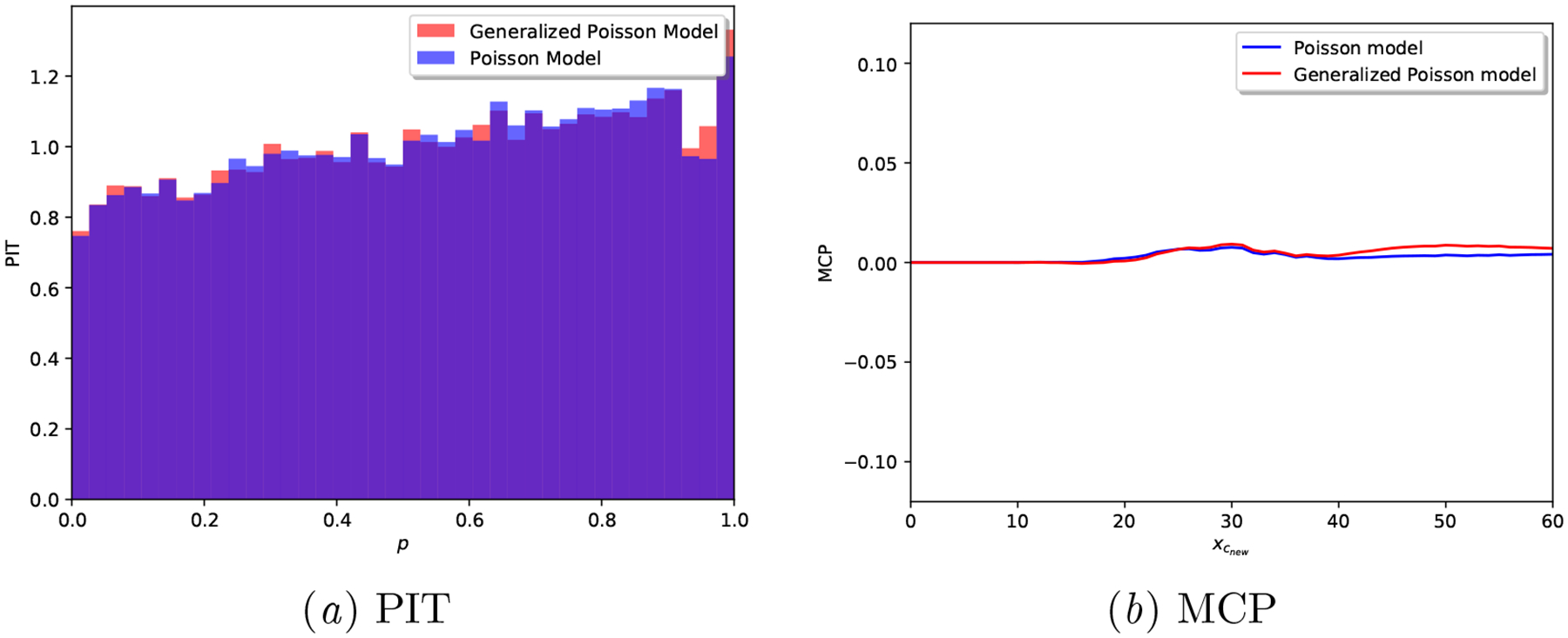
Synthetic Poisson: Calibration plots for a realization of each model.

Table 6:

Posterior predictive width at day 0 of next cycle.

Model	Interval Width for (1 – α) posterior mass.
	(1 – α) = 0.2	(1 – α) = 0.5	(1 – α) = 0.8
Poisson model	3.208 (± 0.006)	8.757 (± 0.027)	21.060 (± 0.167)
Proposed model	3.211 (± 0.010)	8.786 (± 0.030)	21.182 (± 0.392)

B.2. Generalized Poisson generative model of cycle lengths

Data generating process.

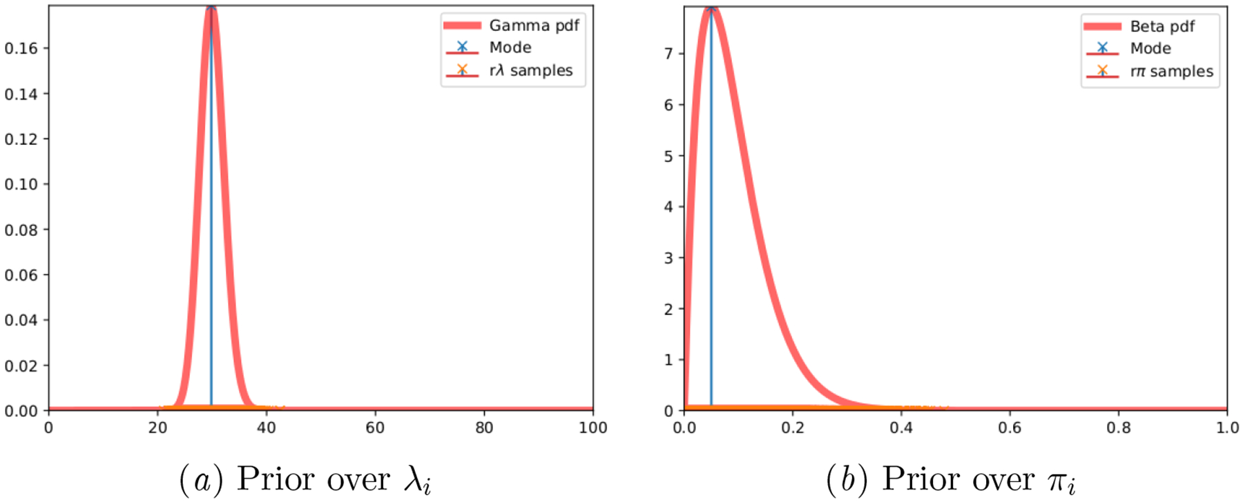
The observed cycle lengths are drawn from the generative model as proposed in Section 3, where cycle length data is drawn from a Generalized Poisson distribution. The specific hyperparameters used for our simulation are Θ = {κ = 160, γ = 4, α_ξ = 2, β_ξ = 20, α = 2, β = 20}, resulting in parameter priors and per-individual sample draws as illustrated in Figure 10.

Figure 10:

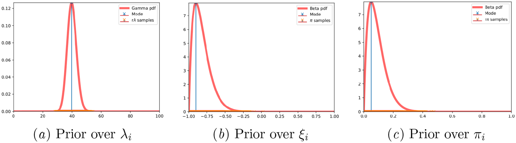
Synthetic Generalized Poisson: Ground truth parameter priors and per-individual drawn samples.

Predictive accuracy and calibration.

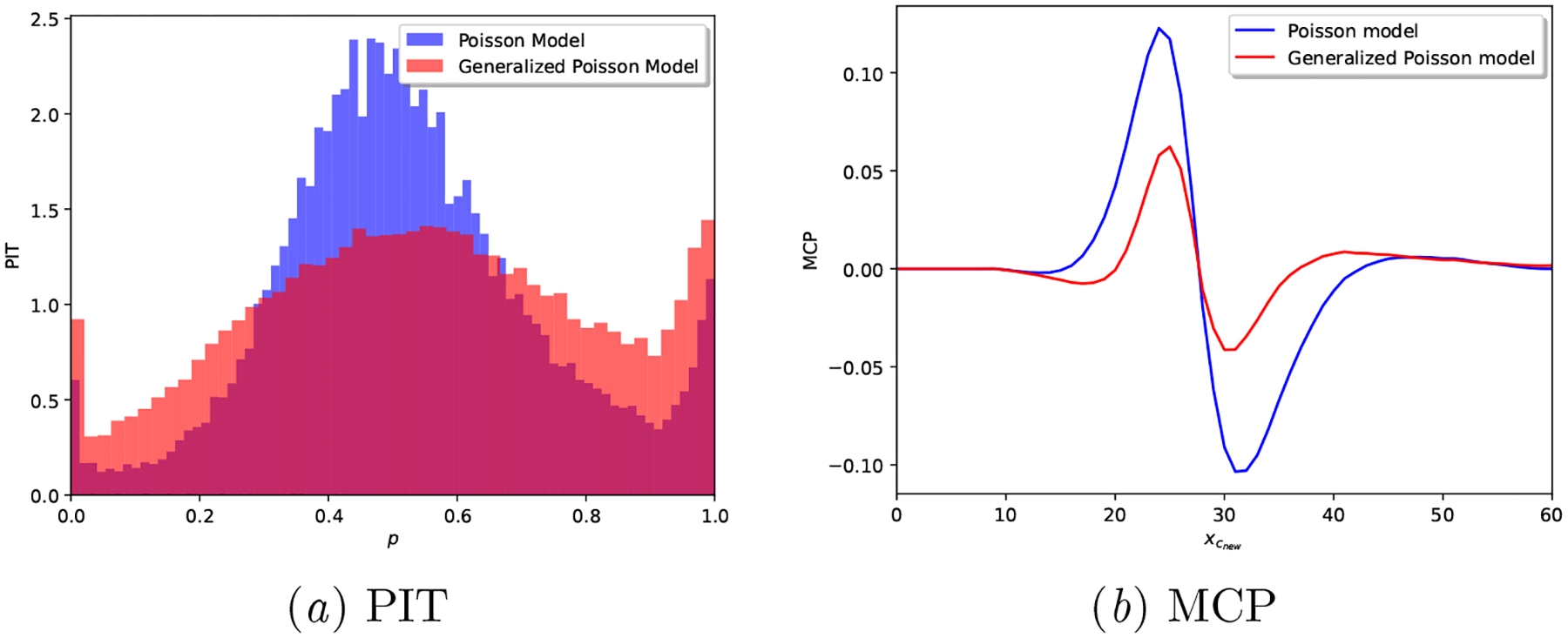
Figures 11 and 12 demonstrate the limitations of the Poisson model when the data generating mechanism is not Poisson distributed: the generated cycle length data in these experiments is drawn from a Generalized Poisson that is under-dispersed (see specific hyperparameters above).

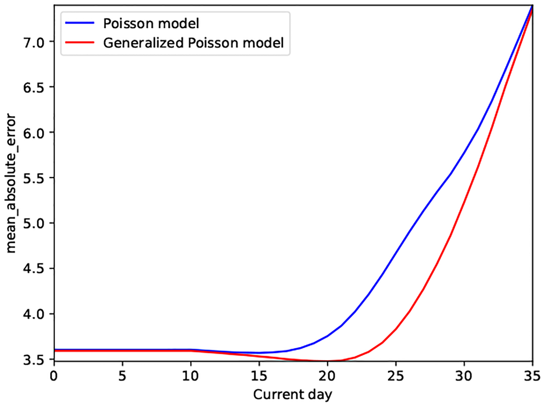
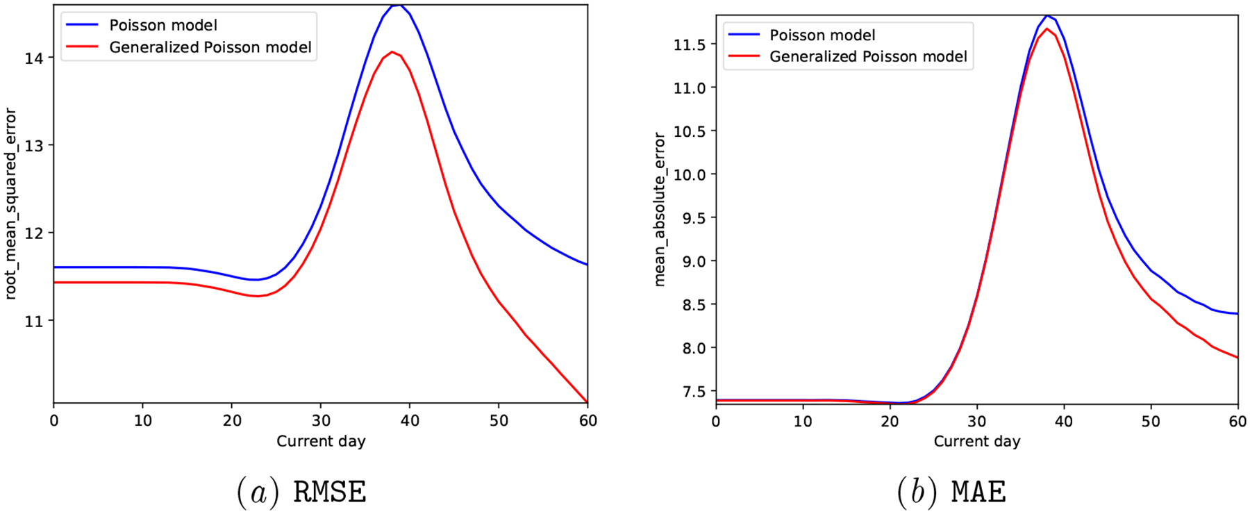
We observe that the Proposed model clearly outperforms the Poisson model both in terms of predictive accuracy (reduced MAE and RMSE in Figure 11) and calibration metrics (Figure 12 and Table 7).

Figure 11:

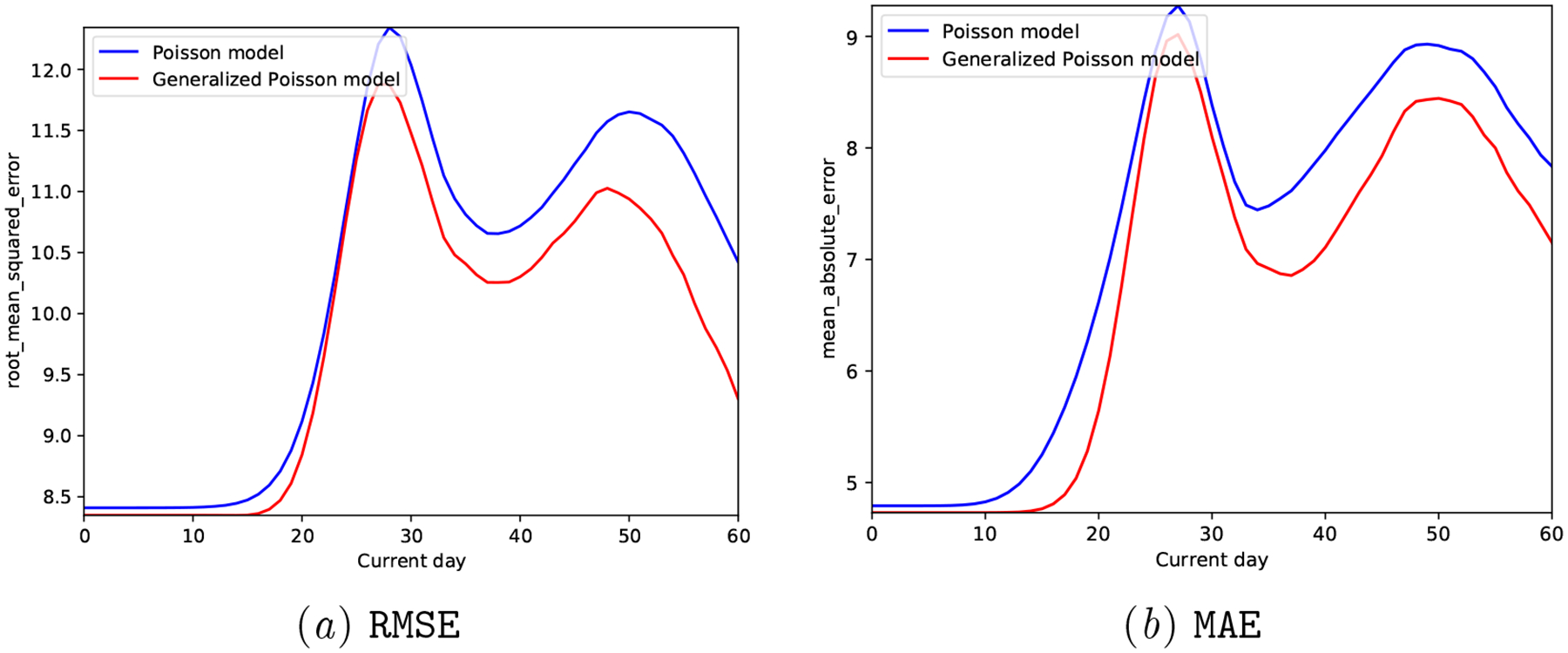
Synthetic Generalized Poisson: Prediction accuracy of the generative models at different days of the next cycle.

In Figure 12, note how the PIT of the Poisson model is hump-shaped, i.e., it is clearly over-dispersed, while the Proposed model’s PIT histogram is close to a uniform distribution. In addition, the MCP plot for the Proposed model hardly deviates from the origin, while the Poisson model showcases a calibration mismatch around $x_{c_{new}}=20$.

Overall, these results validate our claim that a Generalized Poisson based model is able to more flexibly adjust to the uncertainty of observed cycle lengths and provide well-calibrated predictions—all scoring rule results in Table 5 are better for the Proposed model, and their posterior predictive interval width much smaller, see Table 8.

Figure 12:

Synthetic Generalized Poisson: Calibration plots for a realization of each model.

Table 7:

Synthetic Generalized Poisson: Calibration results for the generative models, higher is better

Model	Brier score	Spherical score	Logarithmic score	CRPS
Poisson model	−0.930 (± 0.000)	0.269 (± 0.000)	−2.835 (± 0.001)	−3.553 (± 0.003)
Proposed model	−0.912 (± 0.000)	0.295 (± 0.000)	−2.785 (± 0.001)	−3.385 (± 0.002)

Table 8:

Posterior predictive width at day 0 of next cycle.

Model	Interval Width for (1 – α) posterior mass.
	(1 – α) = 0.2	(1 – α) = 0.5	(1 – α) = 0.8
Poisson model	2.761 (± 0.010)	7.558 (± 0.034)	17.569 (± 0.157)
Proposed model	1.511 (± 0.005)	4.141 (± 0.019)	12.379 (± 0.199)

B.3. Real-world Menstrual mHealth Data

We present predictive results for the models as described in Section 5.1.1 in the real-world cycle length dataset presented in Section 4.

Predictive accuracy and calibration.

Since we have provided evidence in the main manuscript (see Table 2) on the point estimate accuracy of the neural network based alternatives, we hereby focus on their calibration limitations.

Table 9:

Real-world dataset: Calibration results for the studied models, higher is better

Model	Brier score	Spherical score	Logarithmic score	CRPS
CNN	−1.816 (± 0.000)	0.092 (± 0.000)	N/A	−4.274 (± 0.000)
LSTM	−1.790 (± 0.036)	0.105 (± 0.018)	N/A	−3.867 (± 0.168)
RNN	−1.786 (± 0.028)	0.107 (± 0.014)	N/A	−3.914 (± 0.179)
Poisson model	−0.931 (± 0.000)	0.267 (± 0.000)	−3.022 (± 0.000)	−2.921 (± 0.001)
Proposed model	−0.910 (± 0.000)	0.298 (± 0.000)	−2.854 (± 0.000)	−2.740 (± 0.001)

Figure 13:

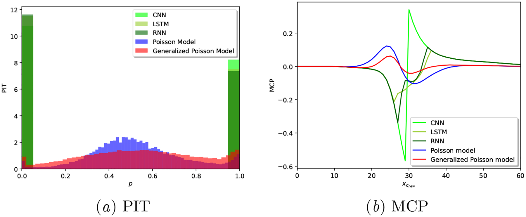
Real-world dataset: Calibration plots for a realization of each model.

Results in Table 9 and Figure 13 show very poor calibration performance of all the neural network based approaches, in alignment with the existing literature on the calibration limitations of these techniques in other applications as well (Guo et al., 2017; Nixon et al., 2019). Note that these results are computed based on the deterministic outputs of these models, i.e., the outputs of the CNN, LSTM and RNN models are point estimates, hence the extreme-valued PIT results in Figure 13(a)subfigure.

We acknowledge that this behavior could be avoided with Bayesian or ensemble-based neural network models that provide probabilistic outputs. However, implementing those alternative models was out of the scope of this work, and we reiterate that there is a growing literature on the calibration shortcomings of these approaches (Wenzel et al., 2020), specially so when approximate inference is used (Foong et al., 2019).

As demonstrated across the variety of considered metrics, we conclude that the Proposed model provides better calibrated results.

Computational complexity.

As explained in Section A.6, the complexity of the training procedure of the proposed Generalized Poisson-based model is determined by the type-II maximum likelihood estimation of model hyperparameters.

We provide in Table 10 details on the number of training epochs (and their corresponding execution times) as executed in an HP Enterprise XL170r E5–2650v4 CPU with 128 GB of RAM memory.

We observe that all models reach convergence within a few number of training epochs (average of 11 epochs for the proposed model). The execution-time overhead incurred by the proposed model results from the aforementioned computation of the normalizing constant in Equation (10). Based on our vectorized implementation, we did not find significant accuracy/execution-time benefits beyond M = 500, s_max = 10, and x_max = 1000 in the presented real-data experiments.

Improving or boosting the implementation of the proposed model, both via optimized numerical computation of the normalizing constant and its parallelized/distributed training, was out of the scope of this work.

Table 10:

Real-world dataset: Training procedure comparison for the studied models.

Model	Number of epochs	Execution time (s)
CNN	4.600 (± 0.800)	6.642 (± 1.660)
LSTM	42.400 (± 13.094)	295.732 (± 104.709)
RNN	25.400 (± 13.336)	74.296 (± 35.354)
Poisson model	5.000 (± 0.632)	393.072 (± 69.404)
Proposed model	11.000 (± 1.265)	36093.951 (± 3804.733)

References

- Alba Ana Carolina, Agoritsas Thomas, Walsh Michael, Hanna Steven, Iorio Alfonso, Devereaux PJ, McGinn Thomas, and Gordon Guyatt. Discrimination and calibration of clinical prediction models: users’ guides to the medical literature. JAMA, 318(14):1377–1384, 2017. [DOI] [PubMed] [Google Scholar]
- Avati Anand, Duan Tony, Zhou Sharon, Jung Kenneth, Shah Nigam H, and Ng Andrew Y. Countdown regression: sharp and calibrated survival predictions. In Uncertainty in Artificial Intelligence, pages 145–155. PMLR, 2020. [Google Scholar]
- Van Calster Ben, Nieboer Daan, Vergouwe Yvonne, De Cock Bavo, Pencina Michael J, and Steyerberg Ewout W. A calibration hierarchy for risk models was defined: from utopia to empirical data. Journal of clinical epidemiology, 74:167–176, 2016. [DOI] [PubMed] [Google Scholar]
- Chen I, Joshi S, Ghassemi Marzyeh, and Ranganath Rajesh. Probabilistic machine learning for healthcare. ArXiv, abs/2009.11087, 2020. [DOI] [PubMed] [Google Scholar]
- Chiazze Leonard, Brayer Franklin T., Macisco John J. Jr., Parker Margaret P., and Duffy Benefict J.. The Length and Variability of the Human Menstrual Cycle. The Journal of the American Medical Association, 203(6):377–380, 1968. [PubMed] [Google Scholar]
- Clue. Clue by BioWink GmbH, Adalbertstraße 7–8, 10999 Berlin, Germany. https://helloclue.com/, 2021. [Google Scholar]
- Consul Prem C. Generalized Poisson distributions: properties and applications. M. Dekker, 1989. [Google Scholar]
- Consul Prem C and Famoye Felix. Generalized poisson distribution. Lagrangian Probability Distributions, pages 165–190, 2006. [Google Scholar]
- Dawid A Philip. The well-calibrated Bayesian. Journal of the American Statistical Association, 77(379):605–610, 1982. [Google Scholar]
- Dawid A Philip. Present position and potential developments: Some personal views statistical theory the prequential approach. Journal of the Royal Statistical Society: Series A (General), 147(2):278–290, 1984. [Google Scholar]
- Diebold Francis X and Mariano Robert S. Comparing predictive accuracy. Journal of Business & economic statistics, 20(1):134–144, 2002. [Google Scholar]
- Dusenberry Michael W., Tran Dustin, Choi Edward, Kemp Jonas, Nixon Jeremy, Jerfel Ghassen, Heller Katherine, and Dai Andrew M.. Analyzing the Role of Model Uncertainty for Electronic Health Records. In Proceedings of the ACM Conference on Health, Inference, and Learning, CHIL ‘20, page 204–213, New York, NY, USA, 2020. [Google Scholar]
- Epstein Daniel A, Lee Nicole B, Kang Jennifer H, Agapie Elena, Schroeder Jessica, Pina Laura R, Fogarty James, Kientz Julie A, and Munson Sean A. Examining Menstrual Tracking to Inform the Design of Personal Informatics Tools. Proceedings of the SIGCHI conference on human factors in computing systems. CHI Conference, 2017:6876–6888, May 2017. [DOI] [PMC free article] [PubMed] [Google Scholar]
- Ferrell Rebecca J, O’Connor Kathleen A, Rodriguez German, Gorrindo Tristan, Holman Darryl J, Brindle Eleanor, Miller Rebecca C, et al. Monitoring reproductive aging in a 5-year prospective study: aggregate and individual changes in steroid hormones and menstrual cycle lengths with age. Menopause, 12:567–757, 2005. [DOI] [PubMed] [Google Scholar]
- Foong Andrew YK, Burt David R, Li Yingzhen, and Turner Richard E. On the expressiveness of approximate inference in bayesian neural networks. arXiv preprint arXiv:1909.00719, 2019. [Google Scholar]
- Fox Sarah and Epstein Daniel A. Monitoring menses: Design-based investigations of menstrual tracking applications. The Palgrave Handbook of Critical Menstruation Studies, pages 733–750, 2020. [PubMed] [Google Scholar]
- Gillon R. Medical ethics: four principles plus attention to scope. BMJ, 309(6948):184, 1994. [DOI] [PMC free article] [PubMed] [Google Scholar]
- Gneiting Tilmann and Raftery Adrian E. Strictly proper scoring rules, prediction, and estimation. Journal of the American statistical Association, 102(477):359–378, 2007. [Google Scholar]
- Gneiting Tilmann, Balabdaoui Fadoua, and Raftery Adrian E. Probabilistic forecasts, calibration and sharpness. Journal of the Royal Statistical Society: Series B (Statistical Methodology), 69(2):243–268, 2007. [Google Scholar]
- Goldstein Mark, Han Xintian, Puli Aahlad, Perotte Adler J, and Ranganath Rajesh. X-CAL: Explicit Calibration for Survival Analysis. arXiv preprint arXiv:2101.05346, 2021. [PMC free article] [PubMed] [Google Scholar]
- Goodfellow Ian, Bengio Yoshua, and Courville Aaron. Deep Learning. MIT Press, 2016. http://www.deeplearningbook.org. [Google Scholar]
- Guo Chuan, Pleiss Geoff, Sun Yu, and Weinberger Kilian Q. On calibration of modern neural networks. In International Conference on Machine Learning, pages 1321–1330. PMLR, 2017. [Google Scholar]
- Han Paul KJ, Klein William MP, and Arora Neeraj K. Varieties of uncertainty in health care: a conceptual taxonomy. Medical Decision Making, 31(6):828–838, 2011. [DOI] [PMC free article] [PubMed] [Google Scholar]
- Harlow Siobán D., Gass Margery, Hall Janet E., Lobo Roger, Maki Pauline, Rebar Robert W., Sherman Sherry, Sluss Patrick M., de Villiers Tobie J., and for the STRAW+10 Collaborative Group. Executive Summary of the Stages of Reproductive Aging Workshop + 10: Addressing the Unfinished Agenda of Staging Reproductive Aging. The Journal of Clinical Endocrinology & Metabolism, 97(4):1159–1168, 04 2012. [DOI] [PMC free article] [PubMed] [Google Scholar]
- Kwon Yongchan, Won Joong-Ho, Kim Beom Joon, and Paik Myunghee Cho. Uncertainty quantification using Bayesian neural networks in classification: Application to biomedical image segmentation. Computational Statistics & Data Analysis, 142:106816, 2020. [Google Scholar]
- Li Kathy, Urteaga Iñigo, Wiggins Chris H., Druet Anna, Shea Amanda, Vitzthum Virginia J., and Elhadad Noémie. Characterizing physiological and symptomatic variation in menstrual cycles using self-tracked mobile health data. Nature Digital Medicine, 3(79), 2020. [DOI] [PMC free article] [PubMed] [Google Scholar]
- Li Kathy, Urteaga Iñigo, Shea Amanda, Vitzthum Virginia J, Wiggins Chris H, and Elhadad Noémie. A generative, predictive model for menstrual cycle lengths that accounts for potential self-tracking artifacts in mobile health data. arXiv preprint arXiv:2102.12439, 2021. Presented at the Machine Learning for Mobile Health Workshop at NeurIPS 2020. [Google Scholar]
- Malinin Andrey and Gales Mark. Predictive uncertainty estimation via prior networks. arXiv preprint arXiv:1802.10501, 2018. [Google Scholar]
- Naeini Mahdi Pakdaman, Cooper Gregory, and Hauskrecht Milos. Obtaining well calibrated probabilities using bayesian binning. In Proceedings of the AAAI Conference on Artificial Intelligence, volume 29, 2015. [PMC free article] [PubMed] [Google Scholar]
- Niculescu-Mizil Alexandru and Caruana Rich. Predicting good probabilities with supervised learning. In Proceedings of the 22nd international conference on Machine learning, pages 625–632, 2005. [Google Scholar]
- Nixon Jeremy, Dusenberry Michael W, Zhang Linchuan, Jerfel Ghassen, and Tran Dustin. Measuring Calibration in Deep Learning. In CVPR Workshops, volume 2, 2019. [Google Scholar]
- Orchard Rosemary. Apple’s Cycle Tracking: A Personal Review. https://www.macstories.net/stories/apples-cycle-tracking-a-personal-review/, November 2019.
- Pierson Emma, Althoff Tim, and Leskovec Jure. Modeling Individual Cyclic Variation in Human Behavior. In Proceedings of the 2018 World Wide Web Conference, WWW ‘18, pages 107–116, Republic and Canton of Geneva, Switzerland, 2018. [DOI] [PMC free article] [PubMed] [Google Scholar]
- Rajkomar Alvin, Oren Eyal, Chen Kai, Dai Andrew M, Hajaj Nissan, Hardt Michaela, Peter J Liu Xiaobing Liu, Marcus Jake, Sun Mimi, et al. Scalable and accurate deep learning with electronic health records. NPJ Digital Medicine, 1(1):1–10, 2018. [DOI] [PMC free article] [PubMed] [Google Scholar]
- Rogers Wendy A and Walker Mary J. Fragility, uncertainty, and healthcare. Theoretical medicine and bioethics, 37(1):71–83, 2016. [DOI] [PubMed] [Google Scholar]
- Rosenblatt Murray. Remarks on a multivariate transformation. The annals of mathematical statistics, 23(3):470–472, 1952. [Google Scholar]
- Siebert Uwe. When should decision-analytic modeling be used in the economic evaluation of health care?, 2003.
- Song Hao, Diethe Tom, Kull Meelis, and Flach Peter. Distribution calibration for regression. In International Conference on Machine Learning, pages 5897–5906. PMLR, 2019. [Google Scholar]
- Soumpasis Ilias, Grace Bola, and Johnson Sarah. Real-life insights on menstrual cycles and ovulation using big data. Human Reproduction Open, 2020(2), 04 2020. [DOI] [PMC free article] [PubMed] [Google Scholar]
- Stevens Richard J and Poppe Katrina K. Validation of clinical prediction models: what does the ”calibration slope” really measure? Journal of clinical epidemiology, 118:93–99, February 2020. [DOI] [PubMed] [Google Scholar]
- Symul Laura, Wac Katarzyna, Hillard Paula, and Salathe Marcel. Assessment of Menstrual Health Status and Evolution through Mobile Apps for Fertility Awareness. bioRxiv, 2018. [DOI] [PMC free article] [PubMed] [Google Scholar]
- Treloar Alan E., Boynton Ruth E., Behn Borghild G., and Brown Byron W.. Variation of the human menstrual cycle through reproductive life. International journal of fertility, 12(1 Pt 2):77–126, 1967. [PubMed] [Google Scholar]
- Urteaga Iñigo, McKillop Mollie, and Elhadad Noémie. Learning endometriosis phenotypes from patient-generated data. npj Digital Medicine, 3(88), 06 2020. [DOI] [PMC free article] [PubMed] [Google Scholar]
- Vach Werner. Calibration of clinical prediction rules does not just assess bias. Journal of clinical epidemiology, 66(11):1296–1301, 2013. [DOI] [PubMed] [Google Scholar]
- Vitzthum Virginia J.. The ecology and evolutionary endocrinology of reproduction in the human female. American Journal of Physical Anthropology, 140(S49):95–136, 2009. [DOI] [PubMed] [Google Scholar]
- Wartella Ellen Ann, Rideout Vicky, Montague Heather, Beaudoin-Ryan Leanne, and Lauricella Alexis Re. Teens, health and technology: A national survey. Media and Communication, 4(3):13–23, 1 2016. [Google Scholar]
- Wenzel Florian, Roth Kevin, Veeling Bastiaan S, Swiatkowski Jakub, Tran Linh, Mandt Stephan, Snoek Jasper, Salimans Tim, Jenatton Rodolphe, and Nowozin Sebastian. How good is the bayes posterior in deep neural networks really? arXiv preprint arXiv:2002.02405, 2020. [Google Scholar]
- Wilson Andrew Gordon. The case for Bayesian deep learning. arXiv preprint arXiv:2001.10995, 2020. [Google Scholar]
- Yao Jiayu, Pan Weiwei, Ghosh Soumya, and Doshi-Velez Finale. Quality of uncertainty quantification for Bayesian neural network inference. arXiv preprint arXiv:1906.09686, 2019. [Google Scholar]