Stochastic differential equation model of Covid-19: Case study of Pakistan

Abstract

In recent years, the world lived a horrible nightmare named the Covid-19 pandemic. It’s changing lifestyle caused the closure of critical establishments like schools, sports halls, companies, etc., as well as causing damage and menace for humanity. Mathematical models are helpful tools for modeling and analysing the infectious disease transmission This article presents a stochastic model of the Covid-19 epidemic for a population with five compartments. We give a numerical analysis of the proposed stochastic model. Also, we compare it with results of the corresponding deterministic model.

Introduction

Recently, the coronavirus pandemic has changed the healthy balance of humanity; the world has known a rapid increase in the number of fatalities. Moreover, the novel coronavirus is a respiratory disease that generally transmits through direct contact with an infected person. However, it also can spread by indirect contact with a virus- infected environment. The hardness degree caused by the infection coronavirus differs from one to another according to immune power. Generally, the syndromes of this disease are chills, weakness, stiffness and loss of smell or taste. According to the report done on 12 October 2021 by World Health Organization, the rate of infection by coronavirus is around 237 655 302, and the number of deaths is 4 846 981 worldwide. The first time when announced the outbreak of a new disease named coronavirus was in December 2019. After a new breed of coronavirus SARS-CoV-2 was discovered in Janvier 2020, the town of Wuhan. It’s spread fastly in all countries and provides a great menace to humanity, caused bringing public life to a halt. Because of Covid 19, universities, sports parks, and high-end establishments shuttered, affecting the countries economies and causing economic harm. Furthermore, increasing multimedia awareness programs about Covid-19’s various can be reduced and controlled. Also, the awareness campaigns play a significant role in urging individuals to take the required measures against the disease, as well as help to refute the fake news about Covid-19 and stressing preventative measures like hand washing and mask use.

In literature, many scholars have adopted mathematic approaches to model the transmission of Covid-19 in different countries. For example, in [1], the authors used the classical deterministic SIR epidemic model to formulate a compatible model for the transmission of Covid-19. In addition, they modeled the process of the propagation of the disease by the convex incidence rate. Khan et al. [2] have presented a fractional-order Covid-19 model by the fractional-order differential equation type. Moreover, they gave a detailed mathematical analysis of the dynamics of the Covid-19 with a case study of Saudi Arabia. A new approach based on piecewise differential and integral operators developed by Atangana and Seda in [3] and prolonger in [4] on the epidemiological fields precisely to modeled the third waves of Covid-19 in Turkey, Spain, and Czechia. In [5], the authors study the dynamics of Covid-19 disease with the fuzzy Caputo approach. In the above-cited works, the authors used deterministic ways to formulate mathematical models of the transmission of Covid-19. Whereas these models have some limitations to describe the reality compared with the stochastic models [6] because the parameters of the system are not constant, but it fluctuates around an average value. In addition, the transmission of epidemics is compatible with randomness because in real-life environmental fluctuations influence the propagation of epidemics. Many works on the application of stochastic calculus in epidemiology have been developed. For example, El Koufi et al. in [7] proposed a stochastic epidemic model with vaccination and nonlinear incidence rate and investigated the asymptotic propriety of the system. In [8], the authors have used a system with Markovian switching to study the change of regimes of a human population divided into three classes Susceptible, Infected, and Recovered. In addition, many works integrated the Lévy processes in deterministic systems to give some degree of realism to this model (see Refs. [6], [9], [10], [11]) and to express the effect of certain phenomena such as earthquakes, volcanoes, tsunami, and pandemic on the dynamics of the system. In [12], the authors have proposed an influential work on the Lotka–Volterra population-driven with Lévy noise. Gao and Wang [13] have studied a stochastic mutualism model integrating the Lévy and Markov processes.

The purpose of this paper is to investigate the effect of white noise on the dynamics of the Covid-19 epidemic. Then, we introduce a stochastic model of Covid-19 that includes the randomness effect, and we discuss numerical conditions for the extinction of the Covid-19 epidemic. The rest of this paper is organized as follows. In Section “Deterministic model”, we presented the deterministic system and its analytical results. The limitations of the deterministic model and the presentation of the stochastic differential equation model existing in Section “Stochastic model”. In Section “Numerical investigation”, numerical simulations of our stochastic model with a brief discussion of the obtained results. Finally, we give a conclusion of the paper and futur investigation in Section “Conclusion”.

Deterministic model

In [14], Li et al. investigated an epidemic model of Covid-19 virus transmission and have divided the population into five groups of individuals, namely, Susceptible $S\left(t\right)$, Exposed $E\left(t\right)$, Infected $I\left(t\right)$, Asymptomatic infected $A\left(t\right)$, Recovered $R\left(t\right)$. They presented their model by the following ordinary differential equations:

$$\left\{\begin{array}{c}\frac{dS\left(t\right)}{dt}=\Lambda -\beta (I\left(t\right)+\eta A\left(t\right))\frac{S\left(t\right)}{N\left(t\right)}-\mu S\left(t\right),\hfill \\ \hfill \\ \frac{dE\left(t\right)}{dt}=\beta (I\left(t\right)+\eta A\left(t\right))\frac{S\left(t\right)}{N\left(t\right)}-(\delta +\mu +{\mu }_0)E\left(t\right),\hfill \\ \hfill \\ \frac{dI\left(t\right)}{dt}=\delta (1-\varpi )E\left(t\right)-(\mu +{\mu }_1+{\gamma }_1)I\left(t\right),\hfill \\ \hfill \\ \frac{dA\left(t\right)}{dt}=\delta \varpi E\left(t\right)-(\mu +{\mu }_2+{\gamma }_2)A\left(t\right),\hfill \\ \hfill \\ \frac{dR\left(t\right)}{dt}={\gamma }_{1}I\left(t\right)+{\gamma }_{2}A\left(t\right)-\mu R\left(t\right),\hfill \end{array}\right)$$ (1)

where $\Lambda$ is the recruitment rate from the population, $\beta$ represents the disease transmission rate, $\eta$ denotes the transmissibility multiple of asymptomatic infection. The parameter $\mu$ is the natural mortality rate. However, The terms $\delta (1-\varpi )$ represent the infection rate of the exposed individuals before a successful incubation period. During the test of individuals, the asymptomatic infections observed for the individuals and its recovery is shown by the rate ${\gamma }_2$, the recovery rate from the symptomatic infection is ${\gamma }_1$. The parameters ${\mu }_0$, ${\mu }_1$ and ${\mu }_2$ represent the disease death rates in the exposed, infected, and asymptomatic infected groups, respectively. The theoretical results are shown in [14] by the following:

System (1) has a basic reproduction number $R_0$ defined by

$$R_0=\frac{\delta \beta (k_2\eta \varpi +k_3(1-\varpi ))}{k_1{k}_2{k}_3},$$

where $k_1=\delta +\mu +{\mu }_0$, $k_2=\mu +{\mu }_1+{\gamma }_1$, $k_3=\mu +{\mu }_2+{\gamma }_2$.

The system (1) has a disease-free equilibrium $E_0$ defined by

$$E_0=\left(\frac{\Lambda }{\mu },0,0,0,0\right).$$

If $R_0>1$, there exists a unique endemic equilibrium $E_{\ast }=\left(S^{\ast },E^{\ast },I^{\ast },\right)\left(A^{\ast },R^{\ast }\right)$ expressed as

$$\left\{\begin{array}{c}{S}^{\ast }=\frac{\Lambda }{{\chi }^{\ast }+\mu },\hfill \\ \hfill \\ E^{\ast }=\frac{{\chi }^{\ast }{S}^{\ast }}{k_1},\hfill \\ \hfill \\ I^{\ast }=\frac{\delta (1-\varpi )E^{\ast }}{k_2},\hfill \\ \hfill \\ A^{\ast }=\frac{\delta \varpi E^{\ast }}{k_3},\hfill \\ \hfill \\ R^{\ast }=\frac{{\gamma }_2{A}^{\ast }+{\gamma }_1{I}^{\ast }}{\mu }.\hfill \end{array}\right)$$ (2)

In addition, they have shown the following analytic results

• 1.If $R_0<1$, then the disease-free equilibrium $E_0$ of Covid-19 model (1) is locally asymptotically stable.
• 2.If $R_0<1$, the disease-free equilibrium $E_0$ of Covid-19 model (2) is globally asymptotically stable.

Stochastic model

In the system (1), the parameters are all deterministic and do not consider the effects of environmental fluctuation and randomness. Whereas, in a biological environment, it is more suitable and reasonable to consider how environmental noise affects the spread of the Covid-19 epidemic. Numerous investigations have shown that environmental fluctuations affect the propagation of an epidemic on the population (see, [7], [8], [11], [12], [13], [15], [16]). Therefore, there are many approaches to consider the random fluctuations in the deterministic systems one of them suppose that the epidemic is subject to some small and standard random fluctuations that can be expressed by white noise. In this paper, in order to examine the effect of environmental noise on the system (1), we suppose that the Covid-19 model (1) is subject to environmental fluctuations and the stochastic perturbations are of white noise type and proportional to the variable. Then, we introduce a stochastic Covid-19 model defined by the following system of stochastic differential equation

$$\left\{\begin{array}{c}\frac{dS\left(t\right)}{dt}=\left(\Lambda -\beta (I\left(t\right)+\eta A\left(t\right))\frac{S\left(t\right)}{N\left(t\right)}-\mu S\left(t\right)\right)dt+{\sigma }_{1}S\left(t\right)d{B}_1\left(t\right),\hfill \\ \hfill \\ \frac{dE\left(t\right)}{dt}=\left(\beta (I\left(t\right)+\eta A\left(t\right))\frac{S\left(t\right)}{N\left(t\right)}-(\delta +\mu +{\mu }_0)E\left(t\right)\right)dt+{\sigma }_{2}E\left(t\right)d{B}_2\left(t\right),\hfill \\ \hfill \\ \frac{dI\left(t\right)}{dt}=\left(\delta (1-\varpi )E\left(t\right)-(\mu +{\mu }_1+{\gamma }_1)I\left(t\right)\right)dt+{\sigma }_{3}I\left(t\right)d{B}_3\left(t\right),\hfill \\ \hfill \\ \frac{dA\left(t\right)}{dt}=\left(\delta \varpi E\left(t\right)-(\mu +{\mu }_2+{\gamma }_2)A\left(t\right)\right)dt+{\sigma }_{4}A\left(t\right)d{B}_4\left(t\right),\hfill \\ \hfill \\ \frac{dR\left(t\right)}{dt}=\left({\gamma }_{1}I\left(t\right)+{\gamma }_{2}A\left(t\right)-\mu R\left(t\right)\right)dt+{\sigma }_{5}R\left(t\right)d{B}_5\left(t\right),\hfill \end{array}\right)$$ (3)

where $B_i\left(t\right)$, $(i=1,2,3,4,5)$ are a standard Brownian motion (see Definition 1) defined on a complete probability space $(\Omega ,\mathcal{F},{\left\{{\mathcal{F}}_t\right\}}_{t\ge 0},\mathbb{P})$ be a complete probability space with a filtration ${\left\{{\mathcal{F}}_t\right\}}_{t\ge 0}$ satisfying the usual conditions (i.e. it is increasing and right continuous while ${\mathcal{F}}_0$ contains all $\mathbb{P}$-null sets), ${\sigma }_i$, $(i=1,2,3,4,5)$ represent the intensity of noise.

Definition 1 [17] —

The positive real-time numbers process ${\left(B\left(t\right)\right)}_{t\ge 0}$ is called the Wiener process if

• 1.$B\left(0\right)=0$, $\mathbb{P}-a.s$.
• 2.$\forall 0\le s<t$, $B\left(t\right)-B\left(s\right)$ are independent of ${\mathcal{F}}_s$.
• 3.$\forall 0\le s<t$, $B\left(t\right)-B\left(s\right)\backsim \mathcal{N}(0,t-s)$.

The n-dimensional stochastic differential equation (briefly, SDE) is defined by:

$$dy\left(t\right)=F(t,y\left(t\right))dt+G(t,y\left(t\right))dB\left(t\right),\text{with}{y}_0=y\left(0\right),$$

where $B\left(t\right)$ is a n-dimensional standard Wiener process, $F$ is the drift coefficient, and $G$ is the diffusion coefficient.

Theorem 1

For any initial value $(S\left(0\right),E\left(0\right),I\left(0\right),A\left(0\right),R\left(0\right))$ $\in$ ${\mathbb{R}}_{+}^5$ , there is a unique solution $(S\left(t\right),E\left(t\right),I\left(t\right),A\left(t\right),R\left(t\right))$ to Eq. (3) on $t\ge 0$ and the solution will remain in ${\mathbb{R}}_{+}^5$ with probability one, namely $(S\left(t\right),E\left(t\right),I\left(t\right),A\left(t\right),R\left(t\right))$ $\in$ ${\mathbb{R}}_{+}^5$ for all $t\ge 0$ almost surely (briefly a.s.).

By using the same steps of proof of Theorem 2.1. in [11] we can prove the above theorem. In the next Section, we will show numerical simulations for the model (3) to show the effect of white noise on the dynamics of the Covid-19 epidemic.

Numerical investigation

To study the dynamics of the model (3), we present numerical simulations by using the Milstein numerical approximation method for the SDE presented in [18]. Then, we can write the system (3) by the following discretized form:

$$\left\{\begin{array}{ccc}\hfill S_{i+1}& \hfill =\hfill & S_i+\left(\Lambda -\beta (I_i\left(t\right)+\eta A\left(t\right))\frac{S_i\left(t\right)}{N_i\left(t\right)}-\mu S_i\left(t\right)\right)\Delta t+{\sigma }_1{S}_i\left(t\right)\sqrt{\Delta t}{\xi }_{1,i}\hfill \\ \hfill & \hfill \hfill & +\frac{{\sigma }_1}{2}{S}_i({\xi }_{1,i}^2-1)\Delta t,\hfill \\ \hfill \\ \hfill E_{i+1}& \hfill =\hfill & E_i+\left(\beta (I_i\left(t\right)+\eta A_i\left(t\right))\frac{S_i\left(t\right)}{N_i\left(t\right)}-(\delta +\mu +{\mu }_0)E_i\left(t\right)\right)\Delta t\hfill \\ \hfill & \hfill \hfill & +{\sigma }_2{E}_i\left(t\right)\sqrt{\Delta t}{\xi }_{2,i}\hfill \\ \hfill \\ \hfill & \hfill \hfill & +\frac{{\sigma }_2}{2}{E}_i({\xi }_{2,i}^2-1)\Delta t,\hfill \\ \hfill \\ \hfill I_{i+1}& \hfill =\hfill & I_i+\left(\delta (1-\varpi )E_i\left(t\right)-(\mu +{\mu }_1+{\gamma }_1)I_i\left(t\right)\right)\Delta t+{\sigma }_3{I}_i\left(t\right)\sqrt{\Delta t}{\xi }_{3,i}\hfill \\ \hfill & \hfill \hfill & +\frac{{\sigma }_3}{2}{I}_i({\xi }_{3,i}^2-1)\Delta t,\hfill \\ \hfill \\ \hfill A_{i+1}& \hfill =\hfill & A_i+\left(\delta \varpi E_i\left(t\right)-(\mu +{\mu }_2+{\gamma }_2)A_i\left(t\right)\right)\Delta t+{\sigma }_4{A}_i\left(t\right)\sqrt{\Delta t}{\xi }_{4,i}\hfill \\ \hfill & \hfill \hfill & +\frac{{\sigma }_4}{2}{A}_i({\xi }_{4,i}^2-1)\Delta t,\hfill \\ \hfill \\ \hfill R_{i+1}& \hfill =\hfill & R_i+\left({\gamma }_1{I}_i\left(t\right)+{\gamma }_2{A}_i\left(t\right)-\mu R_i\left(t\right)\right)\Delta t+{\sigma }_5{R}_i\left(t\right)\sqrt{\Delta t}{\xi }_{5,i}\hfill \\ \hfill & \hfill \hfill & +\frac{{\sigma }_5}{2}{R}_i({\xi }_{5,i}^2-1)\Delta t,\hfill \end{array}\right)$$ (4)

where $\left\{{\xi }_{u,i},i\ge 0\right\}$ are sequences of random numbers uniformly distributed in $[0,1]$ and $\Delta t$ is a time step. The initial conditions are given as follows: $S\left(0\right)=219698286$, $E\left(0\right)=300000$, $I\left(0\right)=1714$, $A\left(0\right)=R\left(0\right)=0$. In this paper, we choose the parameters of the third wave in Pakistan between March 06, 2021, till April 30, 2021 [14], [19]. According to [19], the total population in Pakistan at $2021$ is $220000000$, and the recruitment number in model (3) is $\Lambda =8903$ per day. The natural mortality rate is $\mu ={(67.7365)}^{-1}$ [19]. In addition, we regrouped the rest of the parameters in Table 1. Then, by simple computation, we have $R_0=1.2044>1$, then there exists an endemic equilibrium to the system (1) which is globally asymptotically stable.

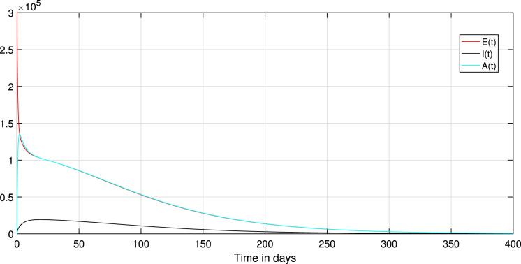
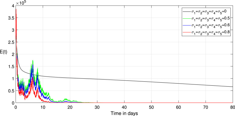
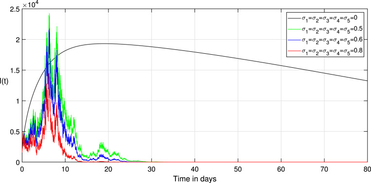
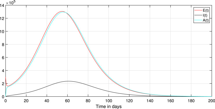
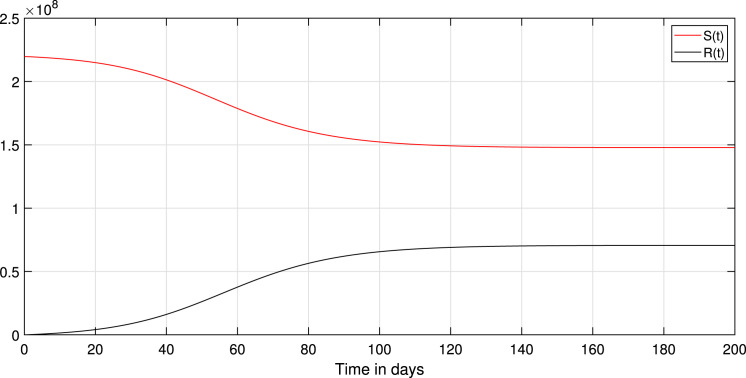
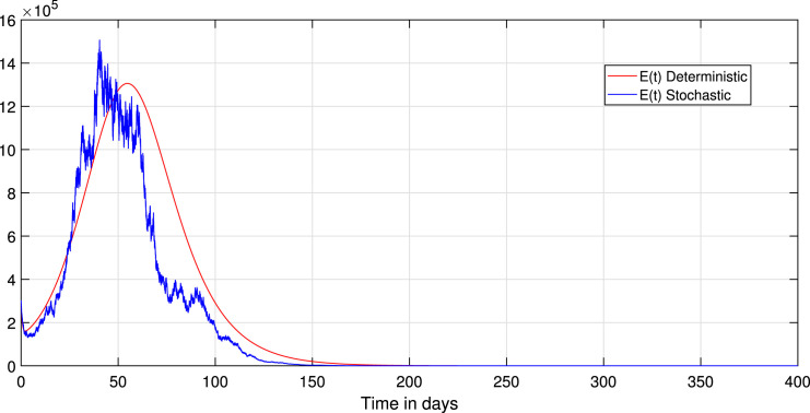
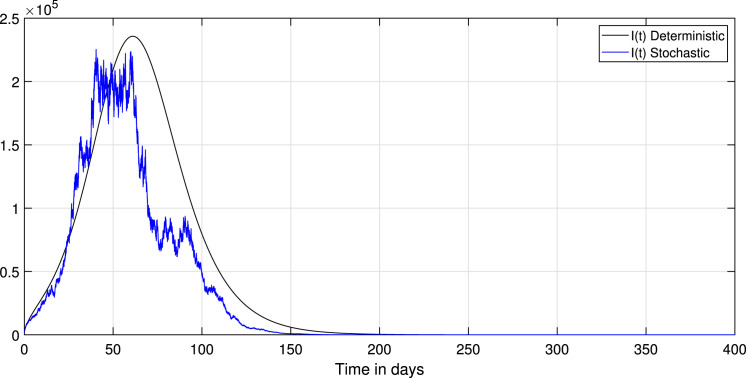
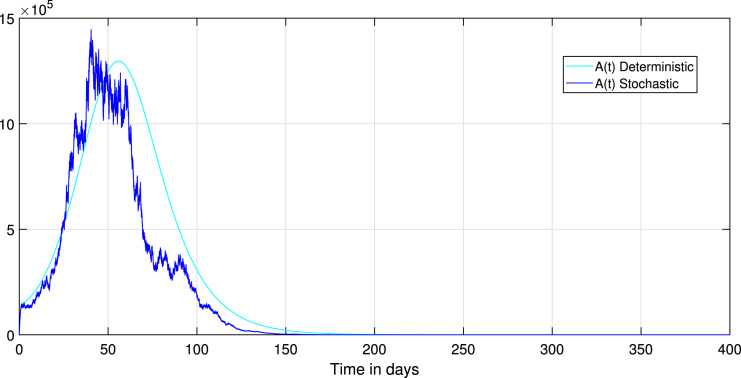
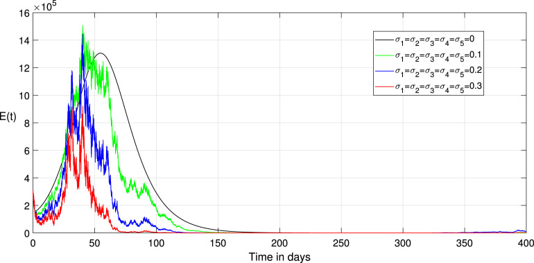
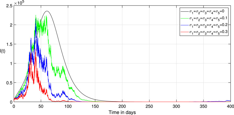
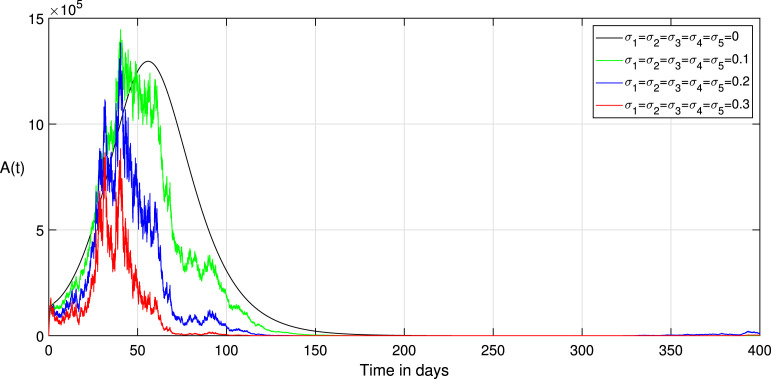
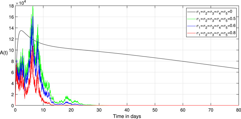
Choosing the value of transmission rate of Covid-19 equal to 0.792, we obtain that $R_0=0.9989\le 1$, then the disease-free equilibrium of system (1) is globally asymptotically stable Fig. 3 confirms this remark. In addition, all values less than 0.792 lead to obtaining a value less than one of the basic reproduction numbers of the system (1). Thus, the coefficient $\beta$ can likewise decrease if we reduce the contact between the infected and susceptible groups. Therefore, we keep the same parameters values used with $\beta =0.792$, and to study the effect of the environmental fluctuation on the dynamics of Covid-19, choosing the different white noise values as: ${\sigma }_i=0$, ${\sigma }_i=0.5$, ${\sigma }_i=0.6$, ${\sigma }_i=0.8$. The integration of white noise in the Covid-19 system leads to the extinction of the epidemic. Then, increasing the white noise value leads to the disappearance of disease (see, Fig. 4, Fig. 5). In addition, the $E\left(t\right)$, $I\left(t\right)$ and $A\left(t\right)$ in system (3) going extinct rapidly comparing with $E\left(t\right)$, $I\left(t\right)$ and $A\left(t\right)$ in a deterministic system (1). On the other hand, when $R_0=1.2044>1$ (see, Fig. 1, Fig. 2). We compare in this situation the dynamics on the stochastic system (3) with the corresponding deterministic system (1) for this taking the noise valued on the system (3) as follows: ${\sigma }_1=0.3$, ${\sigma }_2=0.3$, ${\sigma }_2=0.3$, ${\sigma }_4=0.3$, ${\sigma }_5=0.3$. So, the result of the computer running presented in Fig. 7, Fig. 8, Fig. 9 shows that the integration of the random noise in the system leads to the extinction and the reduction of the Infected, Exposed, and Asymptomatic infected individuals. Moreover, by taking the following different noise values in the system (3): ${\sigma }_i=0$, ${\sigma }_i=0.1$, ${\sigma }_i=0.2$, ${\sigma }_i=0.3$ (i $=$ 1,2,3,4,5) we obtain the graph shown in Fig. 10, Fig. 11, Fig. 12. that show the impact of noise intensity in the spread of the Covid-19 epidemic. Then, a large value of noise led to control the propagation of the epidemic (see, Fig. 10, Fig. 11, Fig. 12).

Fig. 3.

Paths of the deterministic systems (1).

Fig. 4.

Comparison between the paths of stochastic (3) and deterministic (1) systems with different noise values.

Fig. 5.

Comparison between the paths of stochastic (3) and deterministic (1) systems with different noise values.

Fig. 1.

Paths of the deterministic systems (1).

Fig. 2.

Paths of the deterministic systems (1).

Fig. 7.

Comparison between the paths of stochastic (3) and deterministic (1) systems.

Fig. 8.

Comparison between the paths of stochastic (3) and deterministic (1) systems.

Fig. 9.

Comparison between the paths of stochastic (3) and deterministic (1) systems.

Fig. 10.

Comparison between the paths of stochastic (3) and deterministic (1) systems with different noise values.

Fig. 11.

Comparison between the paths of stochastic (3) and deterministic (1) systems with different noise values.

Fig. 12.

Comparison between the paths of stochastic (3) and deterministic (1) systems with different noise values.

Table 1.

The values for parameters given in model (3).

Parameter	Value
$\Lambda$	14
$\beta$	0.5
$\eta$	0.05
$\mu$	0.1
$\delta$	0.02
$\varpi$	0.1
${\mu }_0$	0.8
${\mu }_1$	0.01
${\mu }_2$	0.02
${\gamma }_1$	0.15
${\gamma }_2$	0.15

Conclusion

In this investigation, we presented a stochastic differential equation mathematical model to study the dynamic of Covid-19 in Pakistan. The proposed model considers five classes; Susceptible, Exposed, Infected, and Asymptomatic infected, Recovered. We have affected an environmental perturbation of white noises type in the model (1). We employed the Milstein numerical approximation method to give a comparison between the model (1), (3). Then, with the help of MATLAB and the data presented in [14], we presented graphs that confirm the power of randomness to reduce the number of infected people of Covid-19. We know that the parameters of the epidemic model can depend on the nature of each environmental regime, so to make the system (3) more realistic, we will integrate the telegraph noise into the (3) system in our future work.

CRediT authorship contribution statement

All the authors have equal contribution in this work.

Uncited references

Fig. 6

Fig. 6.

Comparison between the paths of stochastic (3) and deterministic (1) systems with different noise values.

Declaration of Competing Interest

The authors declare that they have no known competing financial interests or personal relationships that could have appeared to influence the work reported in this paper.

References

- 1.Din R., Algehyne E.A. Mathematical analysis of COVID-19 by using SIR model with convex incidence rate. Results Phys. 2021;23 doi: 10.1016/j.rinp.2021.103970. [DOI] [PMC free article] [PubMed] [Google Scholar]
- 2.Chu Y.M., Ali A., Khan M.A., Islam S., Ullah S. Dynamics of fractional order COVID-19 model with a case study of Saudi Arabia. Results Phys. 2021;21 doi: 10.1016/j.rinp.2020.103787. [DOI] [PMC free article] [PubMed] [Google Scholar]
- 3.Atangana A., Araz S.İ. New concept in calculus: Piecewise differential and integral operators. Chaos Solitons Fractals. 2021;145 [Google Scholar]
- 4.Atangana A., Araz S.İ. medRxiv; Turkey, Spain and Czechia: 2021. Modeling Third Waves of Covid-19 Spread with Piecewise Differential and Integral Operators. [DOI] [PMC free article] [PubMed] [Google Scholar]
- 5.Rahman M., Arfan M., Shah K., Gómez-Aguilar J.F. Investigating a nonlinear dynamical model of COVID-19 disease under fuzzy caputo, random and ABC fractional order derivative. Chaos Solitons Fractals. 2020;140 doi: 10.1016/j.chaos.2020.110232. [DOI] [PMC free article] [PubMed] [Google Scholar]
- 6.El Koufi A., Bennar A., El Koufi N., Yousfi N. Asymptotic properties of a stochastic SIQR epidemic model with Lévy jumps and Beddington–DeAngelis incidence rate. Results Phys. 2021;27 [Google Scholar]
- 7.El Koufi A., Adnani J., Bennar A., Yousfi N. Analysis of a stochastic SIR model with vaccination and nonlinear incidence rate. Int J Differ Equ Appl. 2019;2019 [Google Scholar]
- 8.Greenhalgh D., Liang Y., Mao X. Modelling the effect of telegraph noise in the SIRS epidemic model using Markovian switching. Physica A. 2016;462 [Google Scholar]
- 9.Liu Y., Zhang Y., Wang Q. A stochastic SIR epidemic model with Lévy jump and media coverage. Adv Difference Equ. 2020;2020(1):1–15. doi: 10.1186/s13662-020-2521-6. [DOI] [PMC free article] [PubMed] [Google Scholar]
- 10.Guo X., Sun W. Periodic solutions of stochastic differential equations driven by Lévy noises. J Nonlinear Sci. 2021;31(2):1–39. [Google Scholar]
- 11.EL Koufi A., Adnani J., Bennar A., Yousfi N. Dynamics of a stochastic SIR epidemic model driven by Lévy jumps with saturated incidence rate and saturated treatment function. Stoch Anal Appl. 2021 [Google Scholar]
- 12.Bao J., Mao X., Yin G., Yuan C. Competitive Lotka–Volterra population dynamics with jumps. Nonlinear Anal. Theory, Methods Appl. 2011;74(17):6601–6616. [Google Scholar]
- 13.Gao H., Wang Y. Stochastic mutualism model under regime switching with Lévy jumps. Physica A. 2019;515:355–375. [Google Scholar]
- 14.Li X.P., Wang Y., Khan M.A., Alshahrani M.Y., Muhammad T. A dynamical study of SARS-COV-2: A study of third wave. Results Phys. 2021;29 doi: 10.1016/j.rinp.2021.104705. [DOI] [PMC free article] [PubMed] [Google Scholar]
- 15.Koufi A.E., Bennar A., Yousfi N. Discrete Dynamics in Nature and Society; 2020. Dynamics of a Stochastic SIRS Epidemic Model with Regime Switching and Specific Functional Response. (2020) [Google Scholar]
- 16.Zu L., Jiang D., O’Regan D. Conditions for persistence and ergodicity of a stochastic Lotka–Volterra predator–prey model with regime switching. Commun Nonlinear Sci Numer Simul. 2015;29(1–3):1–11. [Google Scholar]
- 17.Karatzas I., Shreve S. Springer Science & Business Media; 2012. Brownian Motion and Stochastic Calculus (Vol. 113) [Google Scholar]
- 18.Milstein G.N., Tret’yakov M.V. Mean-square numerical methods for stochastic differential equations with small noises. SIAM J Sci Comput. 1997;18(4):1067–1087. [Google Scholar]
- 19.World / countries / pakistan, https://www.worldometers.info/coronavirus/ country/pakistan/.