Classification of Electroencephalogram in a Mouse Model of Traumatic Brain Injury Using Machine Learning Approaches

Abstract

Traumatic Brain Injury (TBI) is highly prevalent, affecting ~1% of the U.S. population, with lifetime economic costs estimated to be over $75 billion. In the U.S., there are about 50,000 deaths annually related to TBI, and many others are permanently disabled. However, it is currently unknown which individuals will develop persistent disability following TBI and what brain mechanisms underlie these distinct populations. The pathophysiologic causes for those are most likely multifactorial. Electroencephalogram (EEG) has been used as a promising quantitative measure for TBI diagnosis and prognosis. The recent rise of advanced data science approaches such as machine learning and deep learning holds promise to further analyze EEG data, looking for EEG biomarkers of neurological disease, including TBI. In this work, we investigated various machine learning approaches on our unique 24-hour recording dataset of a mouse TBI model, in order to look for an optimal scheme in classification of TBI and control subjects. The epoch lengths were 1 and 2 minutes. The results were promising with accuracy of ~80–90% when appropriate features and parameters were used using a small number of subjects (5 shams and 4 TBIs). We are thus confident that, with more data and studies, we would be able to detect TBI accurately, not only via long-term recordings but also in practical scenarios, with EEG data obtained from simple wearables in the daily life.

I. Introduction

Traumatic brain injury (TBI) is defined as an alteration in brain functioning or brain pathology initiated by external impacts, such as blunt trauma, penetrating objects, or blast waves. TBI results in physical brain damage, including tearing injuries of white matter, hematomas, or cerebral edema [1, 2]. Consequently, it leads to a cascade of metabolic events which can cause a secondary brain damage possibly due to the generation of free radicals, inflammatory responses, calcium-mediated damage, mitochondrial dysfunction, to name a few. Expenses on TBI are high in part due to the chronic and persistent symptoms following TBI, one of the most prominent of which are sleep-wake disturbances, which can last weeks to years after a single TBI [3]. Sleep disturbances may consequently lead to cognitive impairment, increased disability, and delayed functional recovery [3].

TBI can be categorized into mild, moderate, or severe levels based on Glasgow Coma Scale (GCS), Loss of Consciousness (LOC), Post-traumatic amnesia (PTA) [4] which are qualitative tests rather than quantitative measures. Previous studies on mild TBI (mTBI) primarily focused on spectral power and feature-driven approaches such as cross-frequency coupling using quantitative electroencephalogram (EEG) analyses [5, 6] within different sleep stages [5, 7].

EEG reflects cortical neuronal activity, thus providing an indication of the neuronal changes in the brain with high temporal resolution. To date, quantitative EEG (qEEG) analysis has been a well-established approach for analyzing neural data for many years. The American Academy of Neurology (AAN) defines qEEG as the mathematical processing of digital EEG to highlight specific waveform components, to transform EEG into a format or domain that elucidates relevant information, or to associate numerical results with EEG data for subsequent review or comparison [8]. Quantitative EEG has been used in analysis and classification of various EEG tasks such sleep staging, motor imagery, visually evoked potentials, and detection tasks such as emotion, seizure and drowsiness. Quantitative EEG analysis has also been widely used to study changes in neural data in the field of neurological disorders, such as attention deficit hyperactivity disorder (ADHD) [9], Alzheimer’s disease [10], Parkinson’s disease [11], to name a few. Recently, machine learning algorithms have been successfully implemented in the same domains for improved performance [12], leveraging some of their prominent advantages such as ability to automatically extract features, lesser need for labeled data and handling of multi-dimensional data. EEG analysis using machine learning-based approaches is thus being considered as a promising technique for various brain-computer interface applications [13]. For TBI, machine learning has been used for studies of mTBI using different modalities such as EEG [14], fMRI [15], and resting state functional network connectivity [16].

Among animal models used for studies of TBI, a compelling mouse model of mTBI, lateral fluid percussion injury (FPI), demonstrates very similar behavioural deficits and pathology to those found in humans suffering from mTBI, including sleep disturbances [5, 17]. Our team has been conducting studies using this model, yielding promising results. In this paper, we study EEG data acquired from the above-mentioned FPI model of mTBI to explore performance of various widely-used rule-based machine learning algorithms as well as convolutional neural networks (CNNs). Different sleep stages, epoch lengths, features and neural network hyper-parameters have been explored to obtain the best results.

I. Methods

A. Mouse Data in Use

Animal data were acquired as previously published [5, 6]. Mice were 10-week old, 25 g, male C57BL/6J mice (Jackson Laboratory). They were housed in a laboratory space maintained at ambient temperature of 23±1°C with a relative humidity of 25±5% and automatically controlled with 12-hour light/12-hour dark cycles and an illumination intensity of ~100 lx. The animals had access to food and water. All experiments were carried out in accordance with the guidelines provided by the National Institutes of Health in the Guide for the Care and Use of Laboratory Animals and approved by the local IACUC committee.

B. Fluid Percussion Injury (FPI) and EEG/EMG Sleep-Wake Recordings

Animals were divided into two groups: TBI and sham. FPI along with EEG/EMG implantation in mice (n=12) was performed as described previously [5]. Once the hub was FPI-induced and monitored till the stage of toe pinch withdrawal reflex, a 20-ms pulse of saline was delivered onto the dura with the pressure level in between 1.4 and 2.1 atm [18, 19]. Shams underwent the same procedure with an exception of fluid pulse and later returned to the home cage. Mice were then connected to recording cables after five days of recovery period. Once the animal adapted, measurement was initiated after 24 hours. In order to maintain stable sleep/wake activity across days baseline sleep was analyzed on the first and fifth days after the 7-day recovery period [6]. The procedure is shown in Fig. 1.

Fig. 1.

Experimental procedure for data acquisition.

The 24-hour recording datasets obtained at a sampling rate of 256 Hz for each animal were analyzed for sleep staging by an experienced and blinded scorer to divide into 4-second epochs of wake (W), non-rapid eye movement (NREM) and rapid eye movement (REM) as previously described [6]. Table I shows number of 1 min and 2 min non-overlapping wake and sleep epochs extracted from each mouse. When EEG data are considered without bifurcating into sleep and wake stages, the number of epochs remains same for all mice which are, 1,440 and 720 epochs for 1 min and 2 min epoch lengths, respectively.

TABLE I.

Number of non-overlapping epochs in different stages for each mice

Mice	Wake		Sleep
	1min	2min	1min	2min
Sham_102	736	352	325	103
Sham_103	637	275	473	192
Sham_104	922	427	324	140
Sham_107	684	316	500	177
Sham_108	780	364	359	118
TBI_102	901	429	326	120
TBI_103	271	81	737	340
TBI_104	207	61	457	162
TBI_106	458	181	664	289

C. Algorithms Used and Assessment

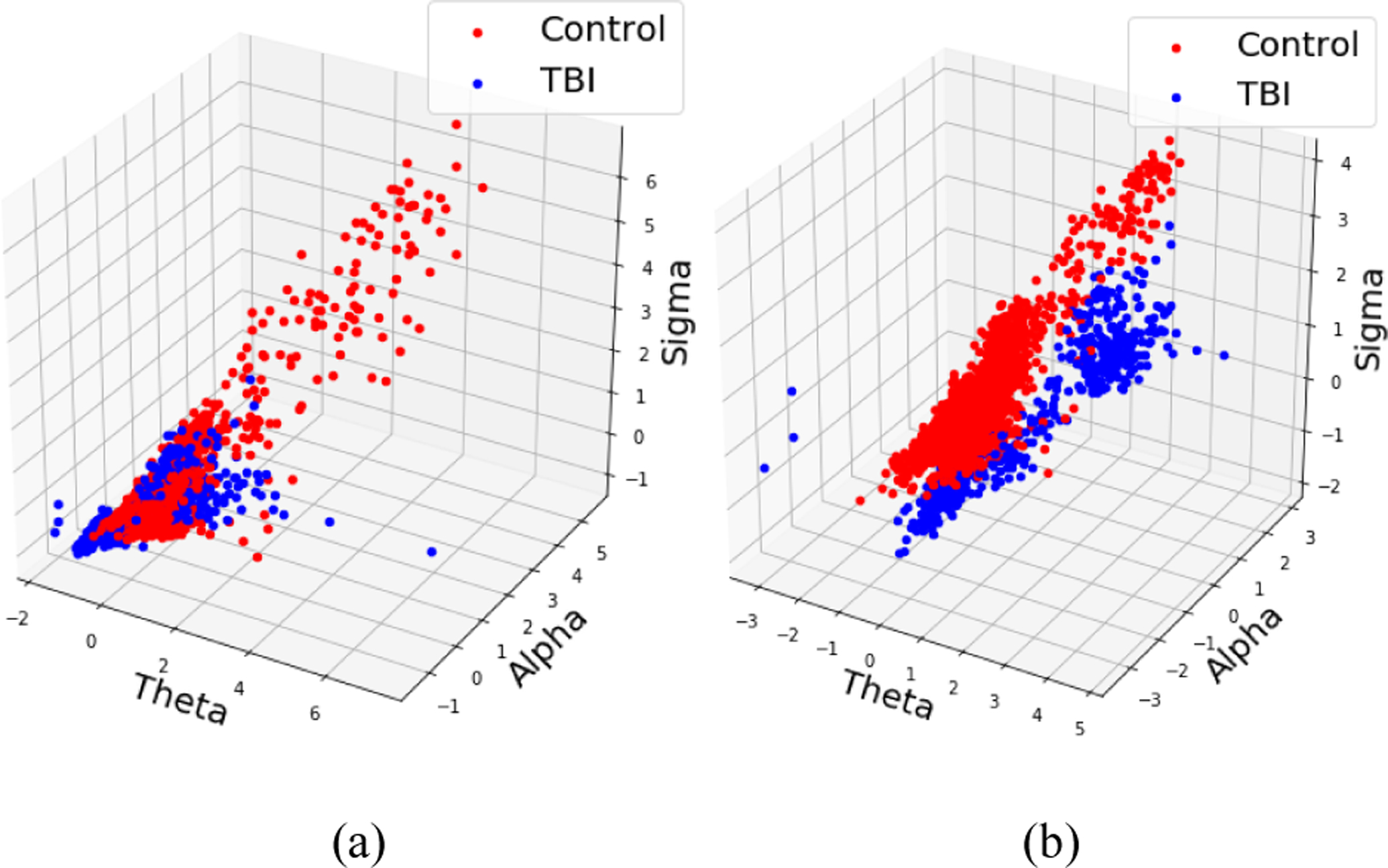
For analysis, 1 min and 2 min non-overlapping wake intervals were extracted from each EEG file. Each epoch was then filtered into different frequency sub-bands: theta (4 – 7.5 Hz), alpha (8 – 12 Hz), sigma (13 – 16 Hz), beta (16.5 – 25 Hz) and gamma (30 – 35 Hz) using a 6^th order Butterworth bandpass digital filter. Average power in each sub-band is calculated for each epoch by calculating power using 256×60 point, 1-D Discrete Fourier Transform (DFT) and taking its mean, which acts as the feature for the rule-based machine learning models. There is need for normalization when the comparison is made across different frequency bands since the power amplitude of frequency specific activity decreases with increase in frequency. Therefore, any slight change in the activity at higher frequencies is overpowered by the activities in the lower frequency bands and cannot be visualized. Fig. 2. represents three of the six features of mice used in training dataset for one trial when 2 min non-overlapping wake epochs were considered. These plots help us visualize the separability between the TBI and sham groups and the need for decibel normalization which is given by

$$\text{dB}=10\times \text{log}10\left\{\frac{\text{activity}}{\text{baseline}}\right\}$$ (1)

Fig. 2.

Feature representation for training dataset (a) without applying decibel normalization (b) with decibel normalization.

The epochs are then feature-normalized to zero mean and unit standard deviation before they are fed to the machine learning algorithms. All normalization parameters calculated for training dataset were used for testing dataset. Python 3.7 along with machine learning tool: scikit-learn was used to implement and test the algorithms. Classification accuracy for ‘K-nearest neighbor’ (KNN) is reported for three values of ‘K’. The ‘Neural network’ is designed with two hidden layers containing 5 nodes each and ‘Support vector machine’ (SVM) uses Radial basis function (rbf) kernel function. All classification accuracy is reported in percentage (%) given by

$$\text{Accuracy}=\frac{\left(\text{True\hspace{0.17em}positives}+\text{True\hspace{0.17em}negatives}\right)}{\text{Total\hspace{0.17em}observations}}\times 100$$ (2)

Machine learning algorithms used are supervised learning algorithms where the target label is already known to the algorithm. ‘Decision tree’ builds tree-structured models incrementally, as it breaks down the training dataset into smaller subsets. ‘Random forest’ takes the majority vote of several decision trees’ prediction which are trained on different parts of the same dataset. ‘Support vector machine’ creates a hyperplane separating the classes by mapping data to a high dimensional feature space. ‘K-nearest neighbor’ algorithm uses similarities in the features to predict the values of the new datapoints based on majority vote of its neighbors with the object being assigned to the class most common among its K-nearest neighbors.

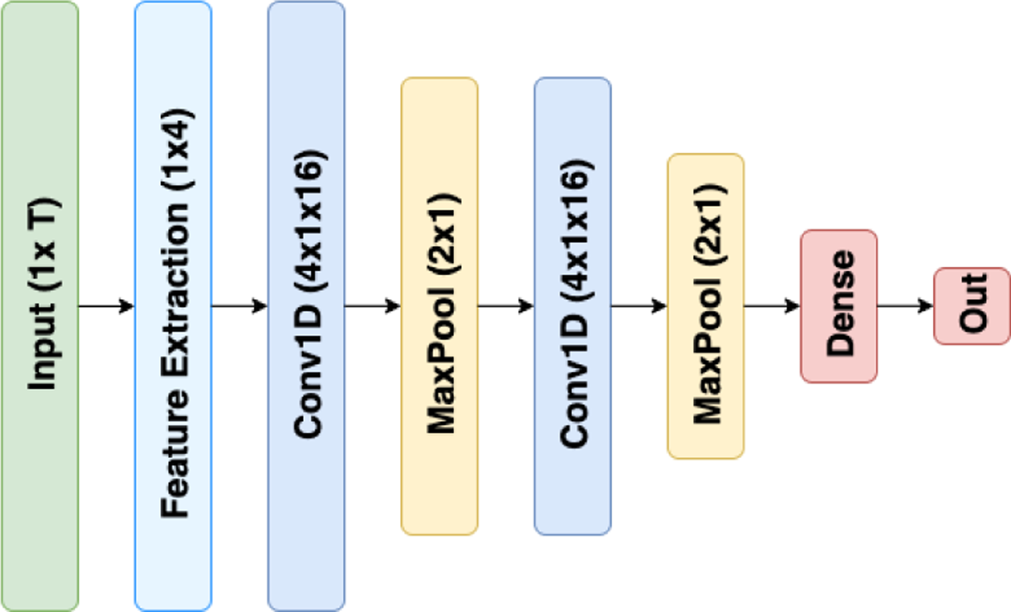
While previously mentioned methods rely on supervised hand-made features to describe data points, there are models designed to take temporal dynamics of the signal into account in a higher resolution. Convolutional Neural Networks (CNN) achieve this by a stack of convolutions, each fed to the next layer. This results in an automatic feature extraction module trained through back-propagation. These networks typically embed pooling layers between two consecutive convolutions and end with a couple of dense layers and finally a classifying softmax layer. This ease of training and accuracy come at the cost of high data dependency. Fig. 3 demonstrates our CNN architecture used in this work which has a standard setting. Initially, a feature extraction layer slides over the raw signal and computes aforementioned 5 average frequency bands. These features are being fed to two layers of conv1d-pool pairs ending with a dense layer and a softmax layer. We used 16 kernels of length 4 for convolutions and strides of 2 for max poolings. The ending dense layer had 40 nodes. Categorical cross entropy cost function trained with Adam optimizer is leveraged under L1 regularization. During CNN hyperparameter tuning, we tried different combinations of kernel lengths (2 to 10), kernel size (2 to 50) and dense layers dimension (10 to 100) in scaled grid search. We also tested architecture with different numbers of convolution layers (up to 6) and noticed that performance is mostly sensitive to the kernel size more than others.

Fig. 3.

The CNN architecture.

II. Results and Discussion

In this section, we present and discuss the results obtained in various scenarios considered for analysis. First, the amount of data which can be accessed by the ML models plays a significant role in the performance of the algorithms due to their inherent working. It is evidenced through several studies that mTBI mice undergo disturbed sleep patterns [20] due to which, they experience inability to stay awake for long bouts of time. Here, fewer bouts of continuous wake epochs were extracted from 24-hour recordings in TBI mice. On the other hand, numbers of sleep epochs were considerably higher in mTBI mice compared to the control group. The number of 1 min and 2 min non-overlapping wake and sleep epochs extracted from each mouse is shown in Table 1. As seen, there is a significant difference in the number of epochs fed to the rule-based ML algorithms in different sleep stages which results in varied classification accuracy.

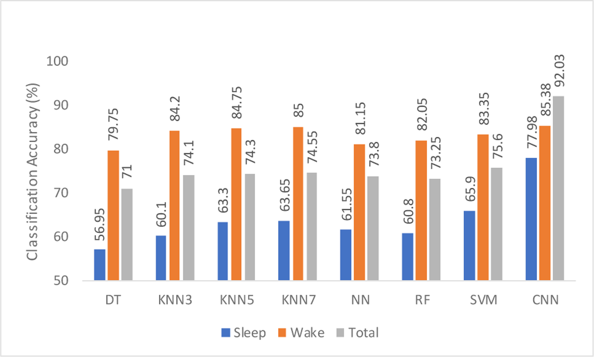
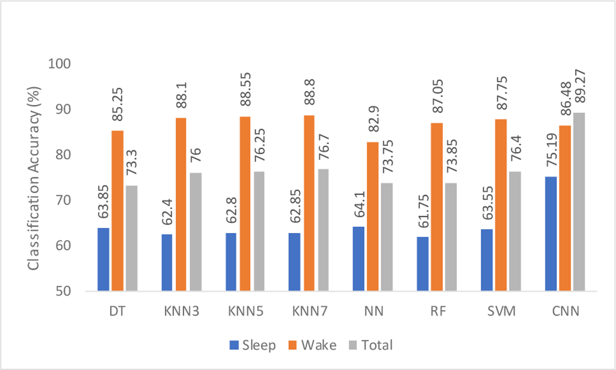
Classification accuracies for different sleep stages are shown in Figs. 4 and 5 for 1 min and 2 min epoch lengths, respectively. It can be seen that the accuracy obtained while using only sleep epochs is low. From Table 1, we can also hypothesize that this may be due to the extremely low number of data points (it is the number of epochs here) that the ML algorithm is trained on. It may also be due to the oversimplification of different sleep stages into one category as “sleep epochs” in our analysis. EEG in different stages of sleep is extremely complex and unique in its own ways which are characterized by different range of dominant frequencies. As a result, combining NREM containing N1, N2 and N3 stages and REM stage into one category and the use of different sub-band power to classify sleep EEG is not an ideal case for analysis. However, owing to its automatic feature selection capability accounting for the temporal dynamics of the EEG signals, CNN outperforms rule-based ML algorithms.

Fig. 4.

Cross-validation accuracy of various classifiers using 1 min epoch lengths of different sleep stages.

Fig. 5.

Cross-validation accuracy of various classifiers using 2 min epoch lengths of different sleep stages.

On the contrary, there are considerably more data points for training during wake stage analysis and therefore, ML models perform better than they do in those cases using sleep stage data. With this, the results obtained for rule-based methods and CNN are comparable. It should be noted that the highest accuracy for 2-min wake stage analysis is obtained by using KNN with ‘K’ value 7, outperforming CNN, which can be explained due to the data extensive approach of CNN models. More detailed analysis on wake stage can be found in our previous work [20]. Overall, the highest classification accuracy of 92.03% was obtained by CNN when the entire EEG signal (both wake and sleep stages) was used with 1-min non-overlapping epochs for the analysis without extraction of various sleep stages. This reiterates the fact that CNN is a data-driven model and usually performs best when there is large amount of data present to train them. It can be observed that for almost all rule-based methods shown in Figs. 4 and 5, the accuracy obtained for the 2-min epoch length is higher. Hence, a careful selection of various parameters such as epoch lengths, features, and others, has to be made while using these ML algorithms.

III. Conclusions

In conclusion, we have successfully demonstrated the use of various machine learning algorithms to classify mTBI data obtained from the mouse model. Rule-based algorithms of decision trees (DT), random forest (RF), neural network (NN), support vector machine (SVM) and K-nearest neighbors (KNN) as well as convolutional neural network (CNN) were conducted to analyze and then compare performance among cases of using only wake data, only sleep data and total data with 1-min and 2-min epoch lengths using average power in different frequency sub-bands as features. The use of CNNs for both sleep and wake data yielded the highest accuracy, indicating a promising method for accurate identification of the relevant brain-based biomarkers in TBI. Combining with other studies of intervention using both animal and human data, this would pave the way to enable appropriate treatment options and allow objective assessment of response to treatment of TBI, which is imperative to addressing this significant socioeconomic problem.

References

- [1].Kenzie ES, Parks EL, Bigler ED, Lim MM, Chesnutt JC, and Wakeland W, “Concussion as a multi-scale complex system: an interdisciplinary synthesis of current knowledge,” Frontiers in neurology, vol. 8, p. 513, 2017. [DOI] [PMC free article] [PubMed] [Google Scholar]
- [2].Kenzie ES, Parks EL, Bigler ED, Wright DW, Lim MM, Chesnutt JC, et al. , “The dynamics of concussion: mapping pathophysiology, persistence, and recovery with causal-loop diagramming,” Frontiers in neurology, vol. 9, p. 203, 2018. [DOI] [PMC free article] [PubMed] [Google Scholar]
- [3].Sandsmark DK, Elliott JE, and Lim MM, “Sleep-wake disturbances after traumatic brain injury: synthesis of human and animal studies,” Sleep, vol. 40, 2017. [DOI] [PMC free article] [PubMed] [Google Scholar]
- [4].Me ON, K C, D S, and et al. (2013). Complications of Mild Traumatic Brain Injury in Veterans and Military Personnel: A Systematic Review. Available: https://www.ncbi.nlm.nih.gov/books/NBK189785/ [PubMed]
- [5].Lim MM, Elkind J, Xiong G, Galante R, Zhu J, Zhang L, et al. , “Dietary therapy mitigates persistent wake deficits caused by mild traumatic brain injury,” Science translational medicine, vol. 5, pp. 215ra173–215ra173, 2013. [DOI] [PMC free article] [PubMed] [Google Scholar]
- [6].Modarres MH, Kuzma NN, Kretzmer T, Pack AI, and Lim MM, “EEG slow waves in traumatic brain injury: Convergent findings in mouse and man,” Neurobiology of Sleep and Circadian Rhythms, vol. 2, pp. 59–70, 2017/01/01/ 2017. [DOI] [PMC free article] [PubMed] [Google Scholar]
- [7].Arbour C, Khoury S, Lavigne GJ, Gagnon K, Poirier G, Montplaisir JY, et al. , “Are NREM sleep characteristics associated to subjective sleep complaints after mild traumatic brain injury?,” Sleep Medicine, vol. 16, pp. 534–539, 2015/04/01/ 2015. [DOI] [PubMed] [Google Scholar]
- [8].Nuwer M, “Assessment of digital EEG, quantitative EEG, and EEG brain mapping: report of the American Academy of Neurology and the American Clinical Neurophysiology Society,” Neurology, vol. 49, pp. 277–292, 1997. [DOI] [PubMed] [Google Scholar]
- [9].Kuperman S, Johnson B, Arndt S, Lindgren S, and Wolraich M, “Quantitative EEG differences in a nonclinical sample of children with ADHD and undifferentiated ADD,” Journal of the American Academy of Child & Adolescent Psychiatry, vol. 35, pp. 1009–1017, 1996. [DOI] [PubMed] [Google Scholar]
- [10].Schreiter-Gasser U, Gasser T, and Ziegler P, “Quantitative EEG analysis in early onset Alzheimer’s disease: a controlled study,” Electroencephalography and clinical neurophysiology, vol. 86, pp. 15–22, 1993. [DOI] [PubMed] [Google Scholar]
- [11].Klassen B, Hentz J, Shill H, Driver-Dunckley E, Evidente V, Sabbagh M, et al. , “Quantitative EEG as a predictive biomarker for Parkinson disease dementia,” Neurology, vol. 77, pp. 118–124, 2011. [DOI] [PMC free article] [PubMed] [Google Scholar]
- [12].Craik A, He Y, and Contreras-Vidal JL, “Deep learning for electroencephalogram (EEG) classification tasks: a review,” Journal of neural engineering, vol. 16, p. 031001, 2019. [DOI] [PubMed] [Google Scholar]
- [13].Lotte F, Congedo M, Lécuyer A, Lamarche F, and Arnaldi B, “A review of classification algorithms for EEG-based brain–computer interfaces,” Journal of neural engineering, vol. 4, p. R1, 2007. [DOI] [PubMed] [Google Scholar]
- [14].Cao C, Tutwiler RL, and Slobounov S, “Automatic classification of athletes with residual functional deficits following concussion by means of EEG signal using support vector machine,” IEEE transactions on neural systems and rehabilitation engineering, vol. 16, pp. 327–335, 2008. [DOI] [PubMed] [Google Scholar]
- [15].Minaee S, Wang Y, Choromanska A, Chung S, Wang X, Fieremans E, et al. , “A deep unsupervised learning approach toward MTBI identification using diffusion MRI,” in 2018 40th Annual International Conference of the IEEE Engineering in Medicine and Biology Society (EMBC), 2018, pp. 1267–1270. [DOI] [PMC free article] [PubMed] [Google Scholar]
- [16].Vergara VM, Mayer AR, Damaraju E, Kiehl KA, and Calhoun V, “Detection of mild traumatic brain injury by machine learning classification using resting state functional network connectivity and fractional anisotropy,” Journal of neurotrauma, vol. 34, pp. 1045–1053, 2017. [DOI] [PMC free article] [PubMed] [Google Scholar]
- [17].Dixon CE, Lyeth BG, Povlishock JT, Findling RL, Hamm RJ, Marmarou A, et al. , “A fluid percussion model of experimental brain injury in the rat,” vol. 67, p. 110, 1987. [DOI] [PubMed] [Google Scholar]
- [18].McIntosh TK, Vink R, Noble L, Yamakami I, Fernyak S, Soares H, et al. , “Traumatic brain injury in the rat: Characterization of a lateral fluid-percussion model,” Neuroscience, vol. 28, pp. 233–244, 1989/01/01/ 1989. [DOI] [PubMed] [Google Scholar]
- [19].Carbonell WS, Maris DO, McCall T, and Grady MS, “Adaptation of the Fluid Percussion Injury Model to the Mouse,” Journal of Neurotrauma, vol. 15, pp. 217–229, 1998/03/01 1998. [DOI] [PubMed] [Google Scholar]
- [20].Vishwanath M, Jafarlou S, Shin I, Lim MM, Dutt N, Rahmani AM, et al. , “Investigation of Machine Learning Approaches for Traumatic Brain Injury Classification via EEG Assessment in Mice,” MDPI Sensors, 2020. [DOI] [PMC free article] [PubMed] [Google Scholar]