Optimal control analysis of COVID-19 vaccine epidemic model: a case study

Abstract

The purpose of this research is to explore the complex dynamics and impact of vaccination in controlling COVID-19 outbreak. We formulate the classical epidemic compartmental model by introducing vaccination class. Initially, the proposed mathematical model is analyzed qualitatively. The basic reproductive number is computed and its numerical value is estimated using actual reported data of COVID-19 for Pakistan. The sensitivity analysis is performed to analyze the contribution of model embedded parameters in transmission of the disease. Further, we compute the equilibrium points and discussed its local and global stability. In order to investigate the influence of model key parameters on the transmission and controlling of the disease, we perform numerical simulations describing the impact of various scenarios of vaccine efficacy rate and other controlling measures. Further, on the basis of sensitivity analysis, the proposed model is restructured to obtained optimal control model by introducing time-dependent control variables $u_1(t)$ for isolation, $u_2(t)$ for vaccine efficacy and $u_3(t)$ for treatment enhancement. Using optimal control theory and Pontryagin’s maximum principle, the model is optimized and important optimality conditions are derived. In order to explore the impact of various control measures on the disease dynamics, we considered three different scenarios, i.e., single and couple and threefold controlling interventions. Finally, the graphical interpretation of each case is depicted and discussed in detail. The simulation results revealed that although single and couple scenarios can be implemented for the disease minimization but, the effective case to curtail the disease incidence is the threefold scenario which implements all controlling measures at the same time.

Introduction

COVID-19 is an infectious disease caused by a novel coronavirus that affects the human respiratory system. Initially, it was reported in Wuhan city of China, in December 2019. The disease spread very quickly to the rest of the world and caused a million deaths. Certain factors are responsible for the spreading of the infection such as social contacts, sneezing and breath of an infected individual. Due to its uncertain dynamics, it was difficult to control the disease [1]. To reduce infection transmission different countries use different strategies and most of them follow common policies, such as social distances and self-quarantine. Researchers around the world are focusing on giving some useful strategies to overcome this COVID-19 epidemic. Vaccination is an effective controlling measure that to protect against infectious disease. Vaccination along with the strict implementation of non-pharmaceutical interventions play an important role to put down the burden of COVID-19 infection around the world. In order to explore the complex dynamics of the ongoing pandemic, different approaches have been made. In this scenario, mathematical models are one of the considerable tools and have been used effectively to present various aspects of COVID-19.

Several epidemic models have been developed to study the dynamics of COVID-19. For instance, Li and Zhang [2] investigated an epidemic model to examine the transmission pattern of coronavirus infectious disease with nonlinear contact as well as recovery rates. An extended SEIR model was proposed by Ghostine et al. [3], to observe the transmission of coronavirus COVID-19 in Saudi Arabia. The aim of the proposed study was to analyze the vaccination impact on coronavirus. Fractional mathematical modeling approach provides deeper insights into the dynamics of a phenomena including infectious diseases and its application can be found in [4–6]. To analyze the effects of quarantine, self-isolation and environmental load, a mathematical model was presented Mohammed et al. [5]. A nonlinear system of differential equations for the transmission of COVID-19 dynamics in Algeria was presented Yacine et al. [6]. The authors carried out stability analysis and provide numerical simulation in order to predict the future forecast. Ullah et al. [7, 8] formulated new epidemic models coupled with optimal control problems to study the importance of some specific variable control interventions on the pandemic of COVID-19 in Pakistan and vector-host diseases. The purpose of the study was to explore the transmission pattern as well as to set up possible control strategies to reduce the infection spreading. Yang et al. [9] considered a mathematical model that describes multiple transmission dynamics of COVID-19, and environmental reservoir virus role in the spreading of this disease. Ahmad et al. [10] describe an epidemic model that investigates the spreading pattern of COVID-19 and discussed its application based on the reported number of infected cases by WHO for Pakistan. Incorporating pathogens in the environment and using social distancing factors, a modified epidemic model was presented Samuel et al. [11]. The intention of this study was to predict the future situation of the COVID-19 epidemic, assuming different intervention scenarios that might help to reduce epidemic risk. The optimal control analysis for the outbreak of coronavirus in the USA was carried out by Calvin et al. [12], using SEAIR mathematical model. An epidemic model was designed Takasar et al. [13], that predict future situation based on the number of infected cases and predicted the outcomes on the reported infected cases in Pakistan. The authors carried out sensitivity and optimal control analysis based on the proposed model. It helped to minimize the infection spreading by adopting those precautionary restrictions. Gatyeni et al. [14] formulated an optimal control problem based on an epidemic model using the Pontraygain Maximum Principle. The purpose of the study was to observe the role of joint implementation of social distance, mask usage, actively screening and testing in curtailing the spreading of COVID-19. Omame et al. presented the formulation of a mathematical compartmental model addressing the dynamics of co-infection with COVID-19 in Brazil [15]. The authors in [15] studied the optimal control measures coupled with cost-effective analysis to curtail COVID-19 in the selected region. A similar mathematical analysis with a case study of Malaysia and Nigeria is conducted by Abidemi et al. and Olaniyi et al. in [16, 17], respectively. The authors in [16] considered the actual data reported in Malaysia from 3 March to 31 December of 2020 and parameterized the proposed model. Similarly, in [17], the authors took the cumulative cases between 10 March to 15 July 2020 in order to estimate the model parameters. An epidemic model with a latency period was studied by Liu et al. [18] to analyze the forecast of the data reported in China. An SEIR model was implemented by Suwardi et al. [19], to analyze the spreading pattern of COVID-19 in Indonesia. The authors considered vaccination and isolation as a model key parameters and observed the effect on the transmission of corona-virus. Additionally, many mathematical models were constructed to study the outbreak of COVID-19 in northern African countries, India, Mexico, Italy, Spain, France as well as in Pakistan, the details are presented in Refs. [20–24]. To observe the impact of isolation/quarantine as a control measure of coronavirus transmission, several compartmental epidemic models were developed in Refs. [25, 26]. Khajanchi et al. [27] proposed an extended classical epidemic model with contact and hospitalization strategies to study the COVID-19 outbreak. A time-dependent epidemic model was considered by Singh et al. [28], to analyze the dynamics and critical as well as hospitalized cases.

Keeping in view the above literature review, in the proposed study we discuss the forecast and impact of vaccination in controlling the COVID-19 epidemic based on infected confirm cases in Pakistan, for the period from March 1, 2021 to June 30, 2021. The data for this selected period are chosen because the third wave of COVID-19 started in Pakistan on March 6, 2021. For this purpose, the standard compartmental epidemic model is modified by introducing the vaccination compartment. Initially, the proposed model is examined qualitatively. The elaborated numerical simulations figure out some important model parameters on the transmission of COVID-19. Finally, the optimal control analysis is carried out in order to analyze the impact of different time-dependent controls. The rest of the article is organized as follows. In Sect. 2, mathematical formulation is presented in detail. The qualitative analysis such as positivity and boundedness, biologically feasible region, estimation of parameters, derivation of basic reproductive number as well as stability results are discussed in the third section. The fourth section contains detail about the interpretation of basic reproductive number on model important parameters. Section 5 describes the numerical simulation of the proposed model and provides in the detail some deep insights into the model important parameters on the COVID-19 dynamic as well as the impact of vaccination. In Sect. 6, we present the detail optimal control investigation of the proposed model is discussed in detail. Finally, the work is concluded in Sect. 7, with some useful suggestions.

Mathematical model

We formulate a compartment epidemic model to examine the outbreak of COVID-19 pandemic and the impact of vaccination on transmission and control of disease. To construct the model, at time t total available population is represented by N(t) and grouped into five compartments according to the disease status. The population that can have contact with the infection are placed in the susceptible compartment denoted by S(t). Those exposed to the virus and with no clinical symptoms developed, until complete a latency period are referred to as exposed compartment E(t). The population with fully developed symptoms of coronavirus are infectious and placed in the infected compartment I(t). The compartment V(t), contains the susceptible population with vaccination and finally, the recovered individuals from the infection moved to recovered compartment R(t). Thus,

$$\begin{array}{c}\hfill N(t)=S(t)+E(t)+I(t)+V(t)+R(t).\end{array}$$

Further, we assume that the vaccinated and recovered individuals may have chance to contact with the virus and become susceptible again, therefore they may join the compartment S(t). Based on the assumptions listed above, the transmission phenomena of COVID-19 is stated in form of a nonlinear system of differential equations given by:

$$\begin{array}{cc}\hfill \frac{\mathrm{d}S}{\mathrm{d}t}& =\mathrm{\Theta }-\beta (I+\kappa E)\frac{S}{N}-({\psi }_{\nu }+\mu )S+{\eta }_{\nu }V+\theta R,\hfill \\ \hfill \frac{\mathrm{d}E}{\mathrm{d}t}& =\beta (I+\kappa E)\frac{S}{N}-(\mu +\gamma )E,\hfill \\ \hfill \frac{\mathrm{d}I}{\mathrm{d}t}& =\gamma E-(\mu +{\mu }_0+\omega )I,\hfill \\ \hfill \frac{\mathrm{d}V}{\mathrm{d}t}& ={\psi }_{\nu }S-(\mu +{\eta }_{\nu })V,\hfill \\ \hfill \frac{\mathrm{d}R}{\mathrm{d}t}& =\omega I-(\mu +\theta )R,\hfill \end{array}$$ 1

subject to initial conditions $S(0)\ge 0,E(0)\ge 0,I(0)\ge 0,V(0)\ge 0,R(0)\ge 0.$ In model (1), $\mathrm{\Theta }$ denotes the population recruitment rate and $\mu$ is natural mortality in all compartments. It is further assume that the population in E and I compartments are responsible for the disease transmission where the transmissibly rate of exposed individuals is less than the individuals in I class [29]. The susceptible individuals get infected after interacting with exposed and infected individuals. Therefore, the strength of infection is

$$\begin{array}{c}\hfill \lambda =\beta (I+\kappa E)\frac{S}{N},\end{array}$$

where $\beta$ represent the effective contact rate, $\kappa$ represents relative transmissibility rate. On the other hand, $\gamma$ represents rate of infection development with symptoms, ${\mu }_0$ is death rate due to infection and $\omega$ is rate of recovery from infection. ${\psi }_{\nu }$ denote vaccination rate, ${\eta }_{\nu }$ is vaccine waning rate and $\theta$ is loss of disease-acquired immunity. Hence, model (1) can be written as

$$\begin{array}{cc}\hfill \frac{\mathrm{d}S}{\mathrm{d}t}& =\mathrm{\Theta }-\lambda S-({\psi }_{\nu }+\mu )S+{\eta }_{\nu }V+\theta R,\hfill \\ \hfill \frac{\mathrm{d}E}{\mathrm{d}t}& =\lambda S-(\mu +\gamma )E,\hfill \\ \hfill \frac{\mathrm{d}I}{\mathrm{d}t}& =\gamma E-(\mu +{\mu }_0+\omega )I,\hfill \\ \hfill \frac{\mathrm{d}V}{\mathrm{d}t}& ={\psi }_{\nu }S-(\mu +{\eta }_{\nu })V,\hfill \\ \hfill \frac{\mathrm{d}R}{\mathrm{d}t}& =\omega I-(\mu +\theta )R.\hfill \end{array}$$ 2

Data fitting and parameters estimation procedure

Estimation of the parameters involved in the proposed model from the actual disease incidence data is one of the important analysis and provides an accurate prediction about the infection dynamics. Moreover, to conduct the numerical simulations more realistically, the estimation of parameters from the statistical disease data is significant. This section deals with the estimation procedure using the actual COVID-19 incidence data for a specific period of time (March 1 till June 30, 2021) reported in Pakistan. The parametrization process of the proposed COVID-19 compartmental model developed in (2) is conducted via two approaches. Firstly, the recruitment rate $\mathrm{\Theta }$ as well as the natural mortality rate of population $\mu$ are obtained from the literature mentioned in Table 2. Secondly, rest of the parameters are determined approximately from reported infected cases using the nonlinear least square procedure. The parameters determination procedure is described in detail as follows:

Table 2.

Biological descriptions of system (1) parameters with estimated values

Parameters	Description	Values (per/day)	Source
$\mathrm{\Theta }$	Recruitment rate	8939	Estimated
$\beta$	Effective contact rate	0.4114	Fitted
$\kappa$	Relative transmissibility rate	0.3131	Fitted
$\mu$	Natural mortality rate	$\frac{1}{67.7\times 365}$	[30]
${\mu }_0$	Death rate from disease in I	0.022	[31]
$\gamma$	Transmission from E to I	0.0164	Fitted
${\psi }_{\nu }$	Rate of vaccination	0.0380	Fitted
${\eta }_{\nu }$	Vaccine waning rate	0.0057	Fitted
$\omega$	Recovery rate of infected individuals	0.1000	Fitted
$\theta$	Loss of disease-acquired immunity	0.1762	Fitted

Since on average the lifespan of Pakistani people is 67.7 [30], as a result the estimated natural death rate per day is $\mu =1/(67.7\times 365)$. The birth rate per day, $\mathrm{\Theta }=8939$, is figured out from total population of Pakistan. The remaining parameters are determined from confirmed positive infected cases via the aforementioned statistical approach. The main objective function to be utilized in this procedure is described as follows:

$$\begin{array}{c}\hfill \widehat{\mathrm{\Phi }}=\sum _{\tau =1}^k{({\chi }_{t_{\tau }}-{\tilde{\chi }}_{t_{\tau }})}^2\end{array}$$ 3

where ${\tilde{\chi }}_{t_{\tau }}$ denote the confirmed COVID-19 infected cases, ${\chi }_{t_{\tau }}$ represents solution of the problem described in (1) at time $t_{\tau },$ and k describe the considered actual daily reported cases.

The prediction of the proposed model (1) (depicted with solid plot) to the actual infected cases (depicted by red circles) is shown in Fig. 1. The model simulation in Fig. 1 shows a better agreement with the real data curve. The values of the parameters results from the estimation process are given in Table 1. The initial values of susceptance individuals are considered from [30], while the infected population reported on March 1, 2021, (i.e., $I(0)=1392$) is taken as initial value [31]. Therefore, the resulting estimated value of ${\mathcal{R}}_0$ based on the estimated parameters values is approximately 1.46.

Fig. 1.

Simulation of the data-fitting result for the proposed transmission model (1) to the actual infected cases in Pakistan reported in third wave for the period from March 1, 2021 through June 30, 2021

Table 1.

Biological description of system (1) variables

State variables	Definition
S	Susceptible individuals
E	Exposed individuals
I	Infected individuals
V	Vaccinated individuals
R	Recovered individuals

Model analysis

In this section, we present some fundamental qualitative features of the COVID-19 compartmental model (1). It includes positivity and boundedness, model’s equilibria and their stability analysis. Moreover, an analytical expression for the important epidemiological parameter, termed the basic reproductive number, is provided. The following lemma shows the positivity and boundedness of the system (1) solution.

Positivity and boundedness

Lemma 3.1

Let $\zeta (t)=(S(t),E(t),I(t),V(t),R(t))\in {\mathbf{R}}_{+}^5$ and the initial data $\zeta (0)\ge 0$, then all the solutions of model (1) are nonnegative for all $t>0$. Moreover,

$$\begin{array}{c}\hfill \underset{t\to +\infty }{lim}N(t)\le \frac{\mathrm{\Theta }}{\mu }.\end{array}$$

Proof

Let $\tau =sup\{t>0:\zeta (t)>0\}$ and from the epidemic model (2), we have

$$\begin{array}{c}\hfill \frac{\mathit{dS}}{\mathit{dt}}=\mathrm{\Theta }-(\lambda +{\psi }_{\nu }+\mu )S+{\eta }_{\nu }V+\theta R\ge \mathrm{\Theta }-(\lambda +{\psi }_{\nu }+\mu ),\end{array}$$

can be further expressed as:

$$\begin{array}{c}\hfill \frac{d}{\mathit{dt}}\left(S,(t),exp,\left((\mu +{\psi }_{\nu }),t,+,{\int }_0^t,\lambda ,(\xi ),d,\xi \right)\right)\ge \mathrm{\Theta }\left(exp,\left((\mu +{\psi }_{\nu }),t,+,{\int }_0^t,\lambda ,(\xi ),d,\xi \right)\right),\end{array}$$

by integrating we have,

$$\begin{array}{cc}\hfill S(\tau )& \ge S(0)\left(exp,\left(-,\left((\mu +{\psi }_{\nu }),\tau ,+,{\int }_0^{\tau },\lambda ,(\xi ),d,\xi \right)\right)\right)+exp\left(-,\left((\mu +{\psi }_{\nu }),\tau ,+,{\int }_0^{\tau },\lambda ,(\xi ),d,\xi \right)\right)\hfill \\ \hfill & \times {\int }_0^{\tau }\mathrm{\Theta }\left(exp,\left((\mu +{\psi }_{\nu }),\eta ,+,{\int }_0^{\eta },\lambda ,(\xi ),d,\xi \right)\right)d\eta >0.\hfill \end{array}$$

Similarly, from rest of the equations in the model (2), we obtain desired interpretation following the same procedure.

Hence, it follows that $\zeta (t)=(S(t),E(t),I(t),V(t),R(t))>0$ for all $t>0$. To prove the subsequent part of Lemma (3.1), we have . By adding equations involved in the system (2), we have

$$\begin{array}{cc}\hfill \frac{\mathit{dN}}{\mathit{dt}}& =\mathrm{\Theta }-\mu N-{\mu }_{0}I\hfill \\ \hfill & \le \mathrm{\Theta }-\mu N.\hfill \end{array}$$

By simple manipulation, we have

$$\begin{array}{cc}\hfill N(t)& \le N(0)e^{-\mu t}+e^{-\mu t}{\int }_0^t\mathrm{\Theta }{e}^{-\mu \xi }d\xi \hfill \\ \hfill & \le N(0)e^{-\mu t}+\frac{\mathrm{\Theta }}{\mu }(1-e^{-\mu t}).\hfill \end{array}$$

Thus,

$$\begin{array}{c}\hfill \underset{t\to +\infty }{lim}N(t)\le \frac{\mathrm{\Theta }}{\mu }.\end{array}$$

$\square$

Invariant region

The biological feasible region for the transmission dynamic of COVID-19 epidemic model (1) is given by

$$\begin{array}{c}\hfill \mathrm{\Omega }\subset {\mathbf{R}}_{+}^5,\end{array}$$

where,

$$\begin{array}{c}\hfill \mathrm{\Omega }=\{(S,E,I,V,R)\in {\mathbf{R}}_{+}^5:S+E+I+V+R\le \frac{\mathrm{\Theta }}{\mu }\}.\end{array}$$

Lemma 3.2

The closed region define by $\mathrm{\Omega }\subset {\mathbf{R}}_{+}^5$ is positive invariant for the model (1) with nonnegative initial conditions in ${\mathbf{R}}_{+}^5$.

Proof

As we know that

$$\begin{array}{c}\hfill N(t)=S(t)+E(t)+I(t)+V(t)+R(t),\end{array}$$

then,

$$\begin{array}{cc}\hfill \frac{dN(t)}{\mathit{dt}}& =\mathrm{\Theta }-\mu N(t)-{\mu }_{0}I\hfill \\ \hfill & \le \mathrm{\Theta }-\mu N(t)\hfill \end{array}$$ 4

and

$$\begin{array}{c}\hfill \frac{dN(t)}{\mathit{dt}}\le 0\text{if}N(t)\ge \frac{\mathrm{\Theta }}{\mu }\text{for}t\ge 0,\end{array}$$

but the solution of (4) is

$$\begin{array}{c}\hfill N(t)\le N(0)e^{-\mu t}+\frac{\mathrm{\Theta }}{\mu }(1-e^{-\mu t}).\end{array}$$

Therefore, $N(t)\le \frac{\mathrm{\Theta }}{\mu }$ if $N(0)\le \frac{\mathrm{\Theta }}{\mu }$ as $t\to \infty$. On other hand $N(t)>\frac{\mathrm{\Theta }}{\mu }$ if $N(0)>\frac{\mathrm{\Theta }}{\mu }$ as $t\to \infty$. Thus, the region $\mathrm{\Omega }$ is positive invariant, and all the solutions trajectories are attracted in ${\mathbf{R}}_{+}^5$ $\square$

Disease free equilibrium

The COVID-19 epidemic model (1) has unique disease free and endemic equilibrium points given by ${\mathcal{P}}_0=\left(S_0,,,E_0,,,I_0,,,V_0,,,R_0\right)=\left(\frac{\mathrm{\Theta }(\mu +{\eta }_{\nu })}{\mu (\mu +{\eta }_{\nu }+{\psi }_{\nu })},,,0,,,0,,,\frac{\mathrm{\Theta }{\psi }_{\nu }}{\mu (\mu +{\eta }_{\nu }+{\psi }_{\nu })},,,0\right)$ and ${\mathcal{P}}_{\mathit{EE}}=(S_{\ast },E_{\ast },I_{\ast },V_{\ast },R_{\ast })$, where

$$\begin{array}{c}\hfill \left\{\begin{array}{c}{S}_{\ast }=\frac{\mathrm{\Theta }(\mu +{\eta }_{\nu })M_2}{(\mu +{\eta }_{\nu }+{\psi }_{\nu })[({\mathcal{R}}_0-1)M_1+\mu M_2]},\hfill \\ \hfill \\ E_{\ast }=\frac{\mathrm{\Theta }(\mu +\theta )(\mu +{\mu }_0+\omega )({\mathcal{R}}_0-1)}{({\mathcal{R}}_0-1)M_1+\mu M_2},\hfill \\ \hfill \\ I_{\ast }=\frac{\gamma \mathrm{\Theta }(\mu +\theta )({\mathcal{R}}_0-1)}{({\mathcal{R}}_0-1)M_1+\mu M_2},\hfill \\ \hfill \\ V_{\ast }=\frac{\mathrm{\Theta }{\psi }_{\nu }{M}_2}{(\mu +{\eta }_{\nu }+{\psi }_{\nu })[({\mathcal{R}}_0-1)M_1+\mu M_2]},\hfill \\ \hfill \\ R_{\ast }=\frac{\gamma \omega \mathrm{\Theta }({\mathcal{R}}_0-1)}{({\mathcal{R}}_0-1)M_1+\mu M_2},\hfill \end{array}\right)\end{array}$$

where $M_1=\mu (\mu +\theta )(\mu +\omega )+\mu \gamma (\mu +\omega +\theta )+{\mu }_0(\mu +\gamma )(\mu +\theta )$ and $M_2=(\mu +\theta )(\mu +{\mu }_0+\omega )+\gamma (\mu +\omega +\theta )$.

In subsequent section, the epidemiological threshold parameter known as the basic reproductive number denoted by ${\mathcal{R}}_0$ is derived analytically and discussed the stability analysis in detail for the system (1) equilibria.

The basic reproduction number ${\mathcal{R}}_0$

To calculate ${\mathcal{R}}_0$ the technique of next generation matrix is utilized. We considered E, I and V compartments. The secondary infection in E class is $\beta (I+\kappa E)\frac{S}{N}$, and there is no new infection in I and V. Therefor, $f=[\beta (I+\kappa E)\frac{S}{N},0,0]$, and $v=[(\mu +\gamma )E,-\gamma E+(\mu +{\mu }_0+\omega )I,-{\psi }_{\nu }S+(\mu +{\eta }_{\nu })V]$. Thus, the necessary matrices denoted by and , respectively, at the disease-free equilibrium is given by,

Thus, using the above-mentioned concept, we obtained the following expression of ${\mathcal{R}}_0$

5

where ${\mathcal{R}}_1=\frac{\beta \gamma (\mu +{\eta }_{\nu })}{(\mu +\gamma )(\mu +{\eta }_{\nu }+{\psi }_{\nu })(\mu +{\mu }_0+\omega )}$ and ${\mathcal{R}}_2=\frac{\beta \kappa (\mu +{\eta }_{\nu })}{(\mu +\gamma )(\mu +{\eta }_{\nu }+{\psi }_{\nu })}$.

Stability of disease-free equilibrium

Theorem 3.3

The DFE, ${\mathcal{P}}_0$ is locally asymptotically stable if ${\mathcal{R}}_0<1$ and else unstable.

Proof

The Jacobian of model (1) at DFE, ${\mathcal{P}}_0=\left(\frac{\mathrm{\Theta }(\mu +{\eta }_{\nu })}{\mu (\mu +{\eta }_{\nu }+{\psi }_{\nu })},,,0,,,0,,,\frac{\mathrm{\Theta }{\psi }_{\nu }}{\mu (\mu +{\eta }_{\nu }+{\psi }_{\nu })},,,0\right)$ is,

$$\begin{array}{c}\hfill J({\mathcal{P}}_0)=\left(\begin{array}{ccccc}-\mu -{\psi }_{\nu }& -\frac{\beta \kappa (\mu +{\eta }_{\nu })}{\mu +{\eta }_{\nu }+{\psi }_{\nu }}& -\frac{\beta (\mu +{\eta }_{\nu })}{\mu +{\eta }_{\nu }+{\psi }_{\nu }}& {\eta }_{\nu }& \theta \\ 0& -\gamma -\mu +\frac{\beta \kappa (\mu +{\eta }_{\nu })}{\mu +{\eta }_{\nu }+{\psi }_{\nu }}& \frac{\beta (\mu +{\eta }_{\nu })}{\mu +{\eta }_{\nu }+{\psi }_{\nu }}& 0& 0\\ 0& \gamma & -\mu -{\mu }_0-\omega & 0& 0\\ {\psi }_{\nu }& 0& 0& -\mu -{\eta }_v& 0\\ 0& 0& \omega & 0& -\theta -\mu \end{array}\right)\end{array}$$

and the corresponding characteristic polynomial is

$$\begin{array}{c}\hfill P(\xi )=(-\xi -\theta -\mu )(\xi +\mu )(\xi +\mu +{\eta }_{\nu }+{\psi }_{\nu })(a_2{\xi }^2+a_1\xi +a_0),\end{array}$$ 6

where

$$\begin{array}{cc}\hfill a_2& =1,\hfill \\ \hfill a_1& =\mu +{\mu }_0+\omega +(\gamma +\mu )(1-{\mathcal{R}}_2),\hfill \\ \hfill a_0& =(\gamma +\mu )(\mu +{\mu }_0+\omega )(\mu +{\eta }_{\nu }+{\psi }_{\nu })(1-{\mathcal{R}}_0).\hfill \end{array}$$

The positivity of $a_0$ and $a_1$ is guarantee by ${\mathcal{R}}_0<1$. Thus by Routh–Hurwitz stability criteria for degree two polynomial, the DEF is locally asymptomatically stable in $\mathrm{\Omega }$. $\square$

The global dynamics of DFE, ${\mathcal{P}}_0$ of the COVID-19 epidemic model presented in (1) is explored in the following result.

Theorem 3.4

The disease-free equilibrium ${\mathcal{P}}_0$ is global asymptotically stable if ${\mathcal{R}}_0<1$, otherwise unstable.

Proof

Consider the Lyapunov function of the form

$$\begin{array}{c}\hfill \upsilon (E,I)=E+gI,\text{where}g=\frac{\beta (\mu +{\eta }_{\nu })}{(\mu +{\eta }_{\nu }+{\psi }_{\nu })(\mu +{\mu }_0+\omega )}.\end{array}$$

The Lyapunov derivative is given by:

$$\begin{array}{cc}\hfill \frac{d\upsilon }{\mathit{dt}}& =\frac{\mathit{dE}}{\mathit{dt}}+g\frac{\mathit{dI}}{\mathit{dt}},\hfill \\ \hfill & =\left[\beta ,(I+\kappa E),\frac{S}{N},-,(\mu +\gamma ),E\right]+g\left[\gamma ,E,-,(,\mu ,+,{\mu }_0,+,\omega ,),I\right].\hfill \end{array}$$

Since,

$$\begin{array}{c}\hfill S(t)\le S_0=\frac{\mathrm{\Theta }(\mu +{\eta }_{\nu })}{\mu (\mu +{\eta }_{\nu }+{\psi }_{\nu })}\text{and}N(t)\le \frac{\mathrm{\Theta }}{\mu }\text{then}\frac{S(t)}{N(t)}\le \frac{\mu +{\eta }_{\nu }}{\mu +{\eta }_{\nu }+{\psi }_{\nu }}.\end{array}$$

It follows that

$$\begin{array}{cc}\hfill \frac{d\upsilon }{\mathit{dt}}& \le \left[\kappa ,\frac{\mu +{\eta }_{\nu }}{\mu +{\eta }_{\nu }+{\psi }_{\nu }},+,g,\gamma ,-,(\mu +\gamma )\right]E+\left[\beta ,\frac{\mu +{\eta }_{\nu }}{\mu +{\eta }_{\nu }+{\psi }_{\nu }},-,(\mu +{\mu }_0+\omega ),g\right]I\hfill \\ \hfill & =\left[\beta ,\kappa ,\frac{\mu +{\eta }_{\nu }}{\mu +{\eta }_{\nu }+{\psi }_{\nu }},+,\frac{\beta (\mu +{\eta }_{\nu })}{(\mu +{\eta }_{\nu }+{\psi }_{\nu })(\mu +{\mu }_0+\omega )},\gamma ,-,(\mu +\gamma )\right]E,\hfill \\ \hfill & +\left[\beta ,\frac{\mu +{\eta }_{\nu }}{\mu +{\eta }_{\nu }+{\psi }_{\nu }},-,(\mu +{\mu }_0+\omega ),\frac{\beta (\mu +{\eta }_{\nu })}{(\mu +{\eta }_{\nu }+{\psi }_{\nu })(\mu +{\mu }_0+\omega )}\right]I\hfill \\ \hfill & =(\mu +\gamma )\left[\frac{\beta (\mu +{\eta }_{\nu })(\gamma +\kappa (\mu +{\mu }_0+\omega ))}{(\mu +\gamma )(\mu +{\eta }_{\nu }+{\psi }_{\nu })(\mu +{\mu }_0+\omega )},-,1\right]E,\hfill \\ \hfill & =(\mu +\gamma )[{\mathcal{R}}_0-1]E.\hfill \end{array}$$

Thus, $\frac{d\upsilon }{\mathit{dt}}<0$ if ${\mathcal{R}}_0<1$ and $\frac{d\upsilon }{\mathit{dt}}=0$ if and only if $E(t)=0$. Substituting $E(t)=0$ in (1) leads to $\left(S,(,t,),,,E,(,t,),,,I,(,t,),,,V,(,t,),,,R,(,t,)\right)\to \left(S_0,,,E_0,,,I_0,,,V_0,,,R_0\right)$, as $t\to \infty$. Furthermore, the largest compact invariant set of ${\mathcal{P}}_0$ is $\{(S(t),E(t),I(t),V(t),R(t))\in \mathrm{\Omega }:\frac{d\upsilon }{\mathit{dt}}=0\}$. Hence, by LaSalle’s Invariance Principle, it follows that the disease-free equilibrium point is globally asymptotically stable in $\mathrm{\Omega }$ whenever, ${\mathcal{R}}_0<1$. $\square$

Stability of endemic equilibrium

Theorem 3.5

The ${\mathcal{P}}_{\mathit{EE}}$ is locally asymptotically stable when ${\mathcal{R}}_0>1$. Moreover, ${\mathcal{P}}_{\mathit{EE}}$ is unstable otherwise.

Proof

The Jacobian of system (1) at ${\mathcal{P}}_{\mathit{EE}}=(S_{\ast },E_{\ast },I_{\ast },V_{\ast },R_{\ast })$ is,

$$\begin{array}{c}\hfill J({\mathcal{P}}_{\mathit{EE}})=\left(\begin{array}{ccccc}-{\kappa }_{11}& -{\kappa }_{12}& -{\kappa }_{13}& {\eta }_{\nu }& \theta \\ -{\kappa }_{21}& -{\kappa }_{22}& {\kappa }_{23}& 0& 0\\ 0& \gamma & -{\kappa }_{33}& 0& 0\\ {\psi }_{\nu }& 0& 0& -{\kappa }_{44}& 0\\ 0& 0& \omega & 0& -{\kappa }_{55}\end{array}\right)\end{array}$$ 7

where

$$\begin{array}{cc}\hfill {\kappa }_{11}=& \mu +{\psi }_{\nu }+\lambda ,{\kappa }_{12}=\beta \kappa \frac{\mu S_0}{\mathrm{\Theta }{\mathcal{R}}_0},{\kappa }_{13}=\beta \frac{\mu S_0}{\mathrm{\Theta }{\mathcal{R}}_0},\hfill \\ \hfill {\kappa }_{21}=& \lambda ,{\kappa }_{22}=\mu +\gamma -\beta \kappa \frac{\mu S_0}{\mathrm{\Theta }{\mathcal{R}}_0},{\kappa }_{23}=\beta \frac{\mu S_0}{\mathrm{\Theta }{\mathcal{R}}_0},\hfill \\ \hfill {\kappa }_{33}=& \mu +{\mu }_0+\omega ,{\kappa }_{44}=\mu +{\eta }_{\nu },{\kappa }_{55}=\mu +\theta .\hfill \end{array}$$

The corresponding characteristics equation is,

$$\begin{array}{c}\hfill P(\zeta )={\zeta }^5+b_4{\zeta }^4+b_3{\zeta }^3+b_2{\zeta }^2+b_1\zeta +b_0,\end{array}$$

where

$$\begin{array}{cc}\hfill b_4& =\frac{\mathrm{\Theta }(\mu +\gamma )(\mu +\theta )(\mu +{\mu }_0+\omega )({\mathcal{R}}_0-1)}{\mu M_2{S}_0}+(\mu +\gamma )\left(1,-,\frac{R_2}{{\mathcal{R}}_0}\right)+(\mu +{\mu }_0+\omega ),\hfill \\ \hfill b_3& ={\kappa }_{12}{\kappa }_{21}+{\kappa }_{33}{\kappa }_{44}+({\kappa }_{33}+{\kappa }_{44}){\kappa }_{55}+{\kappa }_{22}({\kappa }_{33}+{\kappa }_{44}+{\kappa }_{55})\hfill \\ \hfill & +{\kappa }_{11}({\kappa }_{22}+{\kappa }_{33}+{\kappa }_{44}+{\kappa }_{55})-(\gamma {\kappa }_{23}+{\eta }_{\nu }{\psi }_{\nu }),\hfill \end{array}$$

$$\begin{array}{cc}\hfill b_2& =\gamma {\kappa }_{13}{\kappa }_{21}+{\kappa }_{22}{\kappa }_{33}({\kappa }_{44}+{\kappa }_{55})+{\kappa }_{44}{\kappa }_{55}({\kappa }_{11}+{\kappa }_{22})+{\kappa }_{12}{\kappa }_{21}({\kappa }_{33}+{\kappa }_{44}+{\kappa }_{55})\hfill \\ \hfill & +{\kappa }_{11}({\kappa }_{33}{\kappa }_{44}+({\kappa }_{33}+{\kappa }_{44}){\kappa }_{55}+{\kappa }_{22}({\kappa }_{33}+{\kappa }_{44}+{\kappa }_{55}))-\gamma {\kappa }_{23}({\kappa }_{11}+{\kappa }_{44}+{\kappa }_{55})\hfill \\ \hfill & -{\eta }_{\nu }{\psi }_{\nu }({\kappa }_{22}+{\kappa }_{33}+{\kappa }_{55}),\hfill \\ \hfill b_1& ={\kappa }_{33}{\kappa }_{44}{\kappa }_{55}({\kappa }_{11}+{\kappa }_{22})+{\kappa }_{11}{\kappa }_{55}({\kappa }_{22}{\kappa }_{33}+({\kappa }_{22}+{\kappa }_{33}){\kappa }_{44}),\hfill \\ \hfill & +{\kappa }_{21}(\gamma {\kappa }_{13}({\kappa }_{44}+{\kappa }_{55})+{\kappa }_{12}({\kappa }_{33}{\kappa }_{44}+{\kappa }_{55}({\kappa }_{33}+{\kappa }_{44})))+\gamma {\eta }_{\nu }{\psi }_{\nu }{\kappa }_{23},\hfill \\ \hfill & -\gamma ({\kappa }_{23}{\kappa }_{44}{\kappa }_{55}+{\kappa }_{11}{\kappa }_{23}({\kappa }_{44}+{\kappa }_{55})+\theta \omega {\kappa }_{21})-{\eta }_{\nu }{\psi }_{\nu }({\kappa }_{22}{\kappa }_{33}-({\kappa }_{22}+{\kappa }_{33}){\kappa }_{55})\hfill \\ \hfill b_0& =\frac{(\mu +\theta )(\mu +{\eta }_{\nu })(\mu +\gamma )(\mu +{\mu }_0+\omega )M_1({\mathcal{R}}_0-1)}{\mu M_2{S}_0}.\hfill \end{array}$$

${\mathcal{R}}_0>1$ ensure that the coefficients $b_4,b_3,b_2,b_1,b_0$ are positive. Further, it is easy to show that the necessary conditions of Routh–Hurwitz stability criteria for degree five polynomial, $b_4{b}_3{b}_2>b_2^2+b_4^2{b}_1$, and $(b_4{b}_1-b_0)(b_4{b}_3{b}_2-b_2^2-b_4^2{b}_1)>b_0{(b_4{b}_3-b_2)}^2+b_1{b}_0^2$ holds. Thus, the $P_{\mathit{EE}}$ is locally asymptotically stable in $\mathrm{\Omega }$. $\square$

Theorem 3.6

The endemic equilibrium point is globally asymptotically stable if ${\mathcal{R}}_0>1$.

Proof

Consider the appropriate Lyapunov function given by (8),

$$\begin{array}{c}\hfill \mathcal{F}(S,E,I,V,R)=\left({\alpha }_1,V_{\ast },-,{\alpha }_2,S_{\ast }\right)ln\left(\frac{S+V}{S_{\ast }+V_{\ast }}\right)-(E_{\ast }+I_{\ast }+R_{\ast })ln\left(\frac{E+I+R}{E_{\ast }+I_{\ast }+R_{\ast }}\right),\end{array}$$ 8

where

$$\begin{array}{c}\hfill {\alpha }_1=\frac{(\mu +\gamma )(\mu +{\eta }_{\nu }+{\psi }_{\nu })}{{\psi }_{\nu }},{\alpha }_2=\frac{\beta (\gamma +\kappa (\mu +{\mu }_0+\omega ))}{\mu +{\mu }_0+\omega },\end{array}$$

then,

$$\begin{array}{cc}\hfill \frac{d\mathcal{F}}{\mathit{dt}}& =\frac{({\alpha }_1{V}_{\ast }-{\alpha }_2{S}_{\ast })}{S+V}\left(\frac{\mathit{dS}}{\mathit{dt}},+,\frac{\mathit{dV}}{\mathit{dt}}\right)-\frac{E_{\ast }+I_{\ast }+R_{\ast }}{E+I+R}\left(\frac{\mathit{dE}}{\mathit{dt}},+,\frac{\mathit{dI}}{\mathit{dt}},+,\frac{\mathit{dR}}{\mathit{dt}}\right).\hfill \end{array}$$

Notice that

$$\begin{array}{cc}\hfill {\alpha }_1{V}_{\ast }-{\alpha }_2{S}_{\ast }& =\frac{\mathrm{\Theta }(\mu +\gamma )M_2(1-{\mathcal{R}}_0)}{({\mathcal{R}}_0-1)M_1+\mu M_2}\hfill \\ \hfill E_{\ast }+I_{\ast }+R_{\ast }& =\frac{\mathrm{\Theta }{M}_2({\mathcal{R}}_0-1)}{({\mathcal{R}}_0-1)M_1+\mu M_2}.\hfill \end{array}$$

Since, S(t), E(t), I(t), V(t), R(t) are all nonnegative for $t>0$, by manipulation we have,

$$\begin{array}{c}\hfill \frac{\mathit{dS}}{\mathit{dt}}+\frac{\mathit{dV}}{\mathit{dt}}\le \mathrm{\Theta }+\theta R\text{and}\frac{\mathit{dE}}{\mathit{dt}}+\frac{\mathit{dI}}{\mathit{dt}}+\frac{\mathit{dR}}{\mathit{dt}}\le \beta (I+\kappa E),\end{array}$$

Therefore,

$$\begin{array}{cc}\hfill \frac{d\mathcal{F}}{\mathit{dt}}& \le \frac{\mathrm{\Theta }{M}_2(1-{\mathcal{R}}_0)}{({\mathcal{R}}_0-1)M_1+\mu M_2}\left(\frac{\mu +\gamma }{S+V},\left(\mathrm{\Theta },+,\theta ,R\right),+,\frac{1}{E+I+R},(\beta (I+\kappa E))\right)\hfill \\ \hfill & \le 0\text{if and only if}{\mathcal{R}}_0>1.\hfill \end{array}$$

Furthermore, $\frac{d}{\mathit{dt}}\mathcal{F}=0$ whenever, ${\mathcal{P}}_{\mathit{EE}}=(S_{\ast },E_{\ast },I_{\ast },V_{\ast },R_{\ast })$. The largest invariant set of $\{{\mathcal{P}}_{\ast }=(S(t),E(t),I(t),V(t),R(t))\in \mathrm{\Omega }:\frac{d}{\mathit{dt}}\mathcal{F}=0\}$ is singleton set $\{{\mathcal{P}}_{\mathit{EE}}\}$. Thus, it follows according to LaSalle’s Invariance Principle that the endemic equilibrium point ${\mathcal{P}}_{\mathit{EE}}$ is globally asymptotically stable in $\mathrm{\Omega }$ whenever ${\mathcal{R}}_0>1$. $\square$

Interpretation of ${\mathcal{R}}_0$ versus model parameters

In this section, we demonstrate graphically the effect of some important COVID-19 model (1) parameters on the ${\mathcal{R}}_0$ as shown in Figs 2, 3, 4 and 5. In Fig. 2, it is observed that with a low vaccination rate ${\psi }_{\nu }$ and higher effective contact rate $\beta$, the value of ${\mathcal{R}}_0$ rises. On the other hand, with the larger value of ${\psi }_{\nu }$, ${\mathcal{R}}_0$ is getting smaller value less than 1. This behavior is due to the opposite sensitivity indices of these parameters. The interpretation of $\kappa$ and ${\psi }_{\nu }$ is observed on ${\mathcal{R}}_0$ in Fig. 3. It is noticed that ${\mathcal{R}}_0$ is significantly decreased with an increased vaccination rate. It means that the increase in vaccination rate effectively decrease ${\mathcal{R}}_0$ and the disease transmission will be minimized. Figure 4 depicts the impact of parameters ${\eta }_{\nu }$ (the vaccine waning rate) and ${\psi }_{\nu }$ (the vaccination rate) on ${\mathcal{R}}_0$. For certain diseases, the immunity wanes over a period of time naturally and susceptible individuals will reinfect. To boost, immunity vaccination is important. In Fig. 4, we noticed that ${\mathcal{R}}_0$ rises with waning of vaccination in susceptible at a higher rate. On the other hand, ${\mathcal{R}}_0$ will reduce providing vaccination to more susceptible will help to boost their immunity and it results in reducing the chances of getting an infection. Figure 5 interprets the effect of contact rate $\beta$ of infected and the relative transmissibility rate $\kappa$ of exposed individuals on ${\mathcal{R}}_0$. It is analyzed that the greater the values of $\beta$ and $\kappa$, the greater will be ${\mathcal{R}}_0$. This behavior is due to the positive sensitivity indices of these parameters. In order to reduce ${\mathcal{R}}_0$, it would be better to impose strict restrictions on social contacts. In Fig. 6, the of behavior parameters $\beta$ and ${\eta }_{\nu }$ on ${\mathcal{R}}_0$ is illustrated. The close observations indicate that the basic reproductive number ${\mathcal{R}}_0$ has an increasing effect with higher $\beta$ and ${\eta }_{\nu }$. It means that the lose of immunity and more social contacts will increase the chances of getting and spreading infection.

Fig. 2.

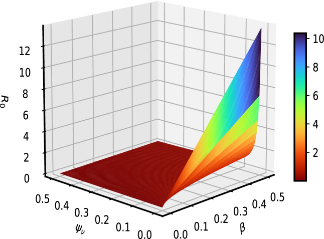
Interpretation of $\beta$ and ${\psi }_{\nu }$ on ${\mathcal{R}}_0$

Fig. 3.

Interpretation of $\kappa$ and ${\psi }_{\nu }$ on ${\mathcal{R}}_0$

Fig. 4.

Interpretation of ${\eta }_{\nu }$ and ${\psi }_{\nu }$ on ${\mathcal{R}}_0$

Fig. 5.

Interpretation of $\beta$ and $\kappa$ on ${\mathcal{R}}_0$

Fig. 6.

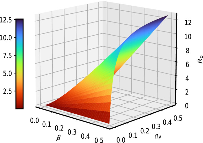
Interpretation of $\beta$ and ${\eta }_{\nu }$ on ${\mathcal{R}}_0$

Numerical simulation and discussion

This section deals with the numerical simulation of epidemic model (1) to examine the complex dynamics as well as the impact of vaccination on transmission and controlling of corona-virus infection. The proposed model is solved numerically using RK4 iterative scheme. The simulation is performed in MATLAB by using initial data $S(0)=220870336,E(0)=50000,I(0)=1392,V(0)=0,R(0)=0$ and the estimated parameters from the reported infected cases in Pakistan, given in Table 2. This section further, describes the interpretation of the impact of some model key parameters on the outbreak of COVID-19 graphically. Figure 7 describes the behavior of symptomatic and exposed individuals with a variation of effective contact rate $\beta$. We have analyzed the impact for the estimated baseline effective contact rate value ($\beta =0.4114$) as well as reduce it by $10\%,20\%$ and $30\%$, respectively. It is noticed that a reasonable decrease is observed in symptomatic as well as in exposed individuals with $30\%$ reduction in effective contact rate to the estimated baseline value. It means that imposing strict restrictions on social contact will reduce the chances of new infective cases. The effect of relative transmissibility rate on infected and exposed population is illustrated in Fig. 8. The behavior is initially observed for the baseline value $\kappa =0.3131$.

Fig. 7.

Impact of effective contact rate $\beta$ on symptomatic and exposed population

Fig. 8.

Impact of transmissibility rate $\kappa$ on symptomatic and exposed population

Furthermore, reducing the baseline value of $\kappa$ by $10\%$, $20\%$ and $30\%$, significant reduction is observed in infected and exposed individuals. The smallest number of infective and exposed individuals is observed with $30\%$ reducing the relative transmissibility rate. It means that increasing the social distancing will reduce the relative transmissibility rate, and it results in a decline the disease transmission. Figure 9 illustrates the impact of vaccination on symptomatic and exposed individuals. Initially, the behavior is observed with estimated baseline value of vaccination rate ${\psi }_{\nu }=0.0380$. By enhancing it with $50\%$ from the baseline value, an effective decrease occurs in both infected and exposed individuals. According to a biological point of view, vaccines contain anti-virus and are responsible to boost the immune system of suspects, and it will increase the recovery rate that is why a decrease is observed in the infected population. The effect of ${\eta }_{\nu }$ (vaccine waning rate) on infected and exposed population is shown in Fig. 10. Firstly, the behavior is analyzed for the estimated baseline value of vaccine waning rate, i.e., ${\eta }_{\nu }=0.0057$. Moreover, $10\%,30\%,50\%$ and $80\%$ reduction in ${\eta }_{\nu }$ to the estimated baseline value shows that infected, as well as exposed populations, will decrease significantly. The lowest peaks are observed in the case of ${\eta }_{\nu }=0.0011$.

Fig. 9.

Impact of vaccination rate ${\psi }_{\nu }$ on symptomatic and exposed population

Fig. 10.

Impact of vaccine waning rate ${\eta }_{\nu }$ on symptomatic and exposed population

Model sensitivity

The sensitivity analysis of basic reproductive number ${\mathcal{R}}_0$ against the model parameters are very important aspects of the presented study. It enables us to figure out the most influential parameters that take place in disease transmission and control. In this section, the sensitivity analysis of various key parameters of COVID-19 model (1) is carried out. The purpose of this procedure is to investigate the importance of model embedded parameters relative to ${\mathcal{R}}_0$. To compute the sensitivity indices, one can take into account the developed formula by Chitnis et al. [32]. The standard sensitivity index of ${\mathcal{R}}_0$ is given by:

$$\begin{array}{c}\hfill S_{\zeta }^{{\mathcal{R}}_0}=\frac{\zeta }{{\mathcal{R}}_0}\frac{\partial {\mathcal{R}}_0}{\partial \zeta },\end{array}$$ 9

where $\zeta$ denotes the model parameters. The partial differentiation of ${\mathcal{R}}_0$ with respect to model parameters is carried out in Mathematica and evaluated its values by using estimated parameters given in Table 2. The calculated indices are given in Table 3. It provides information that how the various parameters are influential to the disease transmission and prevalence. The parameters with positive indices means it has direct dependence on ${\mathcal{R}}_0$, i.e., increasing these parameters will increase ${\mathcal{R}}_0$ and reverse relation exists in case of parameters with negative indices.

Table 3.

Sensitivity indices of ${\mathcal{R}}_0$ to COVID-19 model parameters

Parameters	Sensitivity indices
$\beta$	1
$\kappa$	+ 0.699693
$\mu$	+ 0.0035634
${\mu }_0$	− 0.0541357
$\omega$	− 0.246071
$\gamma$	− 0.697232
${\eta }_{\nu }$	+ 0.862636
${\psi }_{\nu }$	− 0.868761

In Table 3, the parameters with positive indices are $\beta ,\kappa ,\mu$ and ${\eta }_{\nu }$, which means that they have direct effect on ${\mathcal{R}}_0$. It shows that by increasing (or decreasing), these mentioned parameters ${\mathcal{R}}_0$ value will increase (or respectively decrease). On the other hands, parameters ${\mu }_0,\omega ,\gamma$ and ${\psi }_{\nu }$ have negative indices. It indicates the inverse relation with ${\mathcal{R}}_0$ and ultimately, the increase in these parameters will decrease the value of ${\mathcal{R}}_0$ and vice versa. The PRCC values of the selected parameters in the graphical form are shown in Fig. 11.

Fig. 11.

Sensitivity of ${\mathcal{R}}_0$ to embedded parameters of system (1)

Optimal control problem

The impact of isolation, i.e., reduction in effective contacts, enhancement in vaccine efficacy and treatment with constant rates on COVID-19 infectious disease dynamics was analyzed in previous section. In the present section, an optimal control problem is formulated for the mitigation of COVID-19 based on introducing three time-dependent controls denoted by $u_1(t),u_2(t)$ and $u_3(t)$ in the model (1). The purpose of introducing these time-dependent controls is to analyze the effect of its variation with time on the dynamic of COVID-19. The developed control problem is given by (10). The control variable $u_1(t)$ is used for the reduction in effective contacts of expose and infected individuals with susceptible, previously kept constant. To analyze vaccine efficacy enhancement, time-dependent control $u_2(t)$ is introduced, while the control $u_3(t)$ is introduced for enhancement of infection treatment. Thus, the formulated COVID-19 control model is obtained by incorporating the control variables mentioned above is as follows:

$$\begin{array}{cc}\hfill \frac{\mathrm{d}S}{\mathrm{d}t}& =\mathrm{\Theta }-\beta (I+\kappa E)\frac{S}{N}(1-u_1(t))-(u_2(t)+\mu )S+{\eta }_{\nu }V+\theta R,\hfill \\ \hfill \frac{\mathrm{d}E}{\mathrm{d}t}& =\beta (I+\kappa E)\frac{S}{N}(1-u_1(t))-(\mu +\gamma )E,\hfill \\ \hfill \frac{\mathrm{d}I}{\mathrm{d}t}& =\gamma E-(\mu +{\mu }_0+u_3(t))I,\hfill \\ \hfill \frac{\mathrm{d}V}{\mathrm{d}t}& =u_2(t)S-(\mu +{\eta }_{\nu })V,\hfill \\ \hfill \frac{\mathrm{d}R}{\mathrm{d}t}& =u_3(t)I-(\mu +\theta )R,\hfill \end{array}$$ 10

subject to the nonnegative initial conditions. In order to reduce the COVID-19 infection transmission, the cost function

$$\begin{array}{c}\hfill J(u_1,u_2,u_3)={\int }_0^{T_f}\{A_{1}E+A_{2}V+A_{3}I+\frac{1}{2}(A_4{u}_1^2+A_5{u}_2^2+A_6{u}_3^2)\},\end{array}$$ 11

need to be minimized. The constants $A_m$ for $m=1,\dots ,6,$ are used for the balancing cost factors, and $T_f$ represents the final time. Due to nonlinear intervention among the population, quadratic objective functional is take into account, for details see references [7, 8, 15, 16].

The main goal of our observations is to search for optimal control variables $u_i^{\ast }$, for $i=1,2,3$ associated with isolation, efficacy of vaccination and treatment enhancement respectively, such that

The control set corresponding to the problem under consideration is given by

$$\begin{array}{c}\hfill \mathrm{\Omega }=\{(u_1,u_2,u_3):[0,T_f]\to [0,1],(u_1,u_2,u_3)isaLebesguemeasurable\}.\end{array}$$

The Lagrangian and Hamiltonian related to the developed COVID-19 control system (10) is defined as

$$\begin{array}{c}\hfill \mathcal{L}=A_{1}E+A_{2}V+A_{3}I+\frac{1}{2}(A_4{u}_1^2+A_5{u}_2^2++A_6{u}_3^2),\end{array}$$ 12

and

$$\begin{array}{c}\hfill \begin{array}{cc}\hfill \mathcal{H}& =A_{1}E+A_{2}V+A_{3}I+\frac{1}{2}(A_4{u}_1^2+A_5{u}_2^2++A_6{u}_3^2)\hfill \\ \hfill & +{\lambda }_1[\mathrm{\Theta }-\beta (I+\kappa E)\frac{S}{N}(1-u_1(t))-(u_2(t)+\mu )S+{\eta }_{\nu }V+\theta R]\hfill \\ \hfill & +{\lambda }_2[\beta (I+\kappa E)\frac{S}{N}(1-u_1(t))-(\mu +\gamma )E]\hfill \\ \hfill & +{\lambda }_3[\gamma E-(\mu +{\mu }_0+u_3(t))I]\hfill \\ \hfill \\ \hfill & +{\lambda }_4[u_2(t)S-(\mu +{\eta }_{\nu })V]\hfill \\ \hfill \\ \hfill & +{\lambda }_5[u_3(t)I-(\mu +\theta )R],\hfill \end{array}\end{array}$$ 13

where the symbols ${\lambda }_m$, for $m=1,2\dots ,5,$ represent the adjoint variables.

Optimal control solution

To obtain the optimal solution of COVID-19 control problem (10), Pontryagin’s maximum principle [33] is utilized. For this purpose it is assumed that $u_1^{\ast }$, $u_2^{\ast }$ and $u_3^{\ast }$ are desired optimal solution. Therefore, the associated Pontryagin’s maximum principle conditions that will be used in the solution process are as follows:

$$\begin{array}{c}\hfill \left\{\begin{array}{c}\frac{\mathrm{d}z}{\mathrm{d}t}=-\frac{\partial }{\partial {\lambda }_m}\mathcal{H}(t,u_j^{\ast },{\lambda }_m),\hfill \\ \hfill \\ \frac{\partial }{\partial u}\mathcal{H}(t,u_j^{\ast },{\lambda }_m)=0,\hfill \\ \hfill \\ \frac{d{\lambda }_m(t)}{\mathit{dt}}=-\frac{\partial }{\partial z}\mathcal{H}(t,u_j^{\ast },{\lambda }_m).\hfill \end{array}\right)\end{array}$$ 14

The mentioned conditions in (14) has been utilized in the subsequent theorem to get the optimal system solution.

Theorem 6.1

The optimal controls $u_1^{\ast }$, $u_2^{\ast },u_3^{\ast }$ and control system (10) solutions $S^{\ast }$, $E^{\ast }$, $I^{\ast }$, $V^{\ast }$ and $R^{\ast }$ that minimize the objective functional $J(u_1,u_2,u_3)$ over $\mathrm{\Omega }$. Then, there exists adjoint variables ${\lambda }_m$, where $m=1,2,\dots ,5,$ along with transversality conditions ${\lambda }_m(T_f)=0$ such that

$$\begin{array}{cc}\hfill \frac{d{\lambda }_1}{\mathit{dt}}=& \beta (I+\kappa E)\frac{N^{\ast }-S^{\ast }}{N^{\ast 2}}(1-u_1(t))({\lambda }_1-{\lambda }_2)+u_2({\lambda }_1-{\lambda }_4)+{\lambda }_1\mu ,\hfill \\ \hfill \\ \hfill \frac{d{\lambda }_2}{\mathit{dt}}=& -A_1+\beta \frac{(\kappa (N^{\ast }-E^{\ast })-1)S^{\ast }}{N^{\ast 2}}(1-u_1(t))({\lambda }_1-{\lambda }_2)+\gamma ({\lambda }_2-{\lambda }_3)+{\lambda }_2\mu ,\hfill \\ \hfill \\ \hfill \frac{d{\lambda }_3}{\mathit{dt}}=& -A_3+\beta \frac{((N^{\ast }-I^{\ast })-\kappa E^{\ast })S^{\ast }}{N^{\ast 2}}(1-u_1(t))({\lambda }_1-{\lambda }_2)+u_3(t)({\lambda }_3-{\lambda }_5)+{\lambda }_3(\mu +{\mu }_0),\hfill \\ \hfill \\ \hfill \frac{d{\lambda }_4}{\mathit{dt}}=& -A_2+\beta \frac{(I^{\ast }+\kappa E^{\ast })S^{\ast }}{N^{\ast 2}}(1-u_1(t))({\lambda }_2-{\lambda }_1)+{\eta }_{\nu }({\lambda }_4-{\lambda }_1)+{\lambda }_4\mu ,\hfill \\ \hfill \\ \hfill \frac{d{\lambda }_5}{\mathit{dt}}=& \beta \frac{(I^{\ast }+\kappa E^{\ast })S^{\ast }}{N^{\ast 2}}(1-u_1(t))({\lambda }_2-{\lambda }_1)+\theta ({\lambda }_5-{\lambda }_1)+{\lambda }_5\mu .\hfill \end{array}$$

Moreover, the respective optimum controls $u_i^{\ast }$, where $i=1,2,3$ are all present as follows:

$$\begin{array}{c}\hfill \begin{array}{c}{u}_1^{\ast }=\min \{1,\max (\frac{\beta S^{\ast }(I^{\ast }+\kappa E^{\ast })({\lambda }_2-{\lambda }_1)}{A_4{N}^{\ast }},0)\},\hfill \\ \hfill \\ u_2^{\ast }=\min \{1,\max (0,\frac{S^{\ast }({\lambda }_1-{\lambda }_4)}{A_5})\},\hfill \\ \hfill \\ u_3^{\ast }=\min \{1,\max (0,\frac{I^{\ast }({\lambda }_3-{\lambda }_5)}{A_6})\}.\hfill \end{array}\end{array}$$ 15

Proof

The results in (15) are obtained for the Hamiltonian function given in (13), by using transversality conditions and Pontryagin’s maximum principle conditions given in (14). Moreover, the optimal controls $u_1^{\ast }$, $u_2^{\ast }$ and $u_3^{\ast }$ in (15) are computed, by implementing the condition $\frac{\partial \mathcal{H}(t,u_j^{\ast },{\lambda }_m)}{\partial u_j}=0$ given in (14). $\square$

Simulation of the control problem

Numerical simulations of the proposed COVID-19 vaccine model, with control (10) as well as without control (1), are carried out to analyze the usefulness of the indicated preventative measures. A well-known iterative scheme RK4 is used in order to compute the numerical solution of the proposed models. The parameters used in simulation are given in Table 2, while the weights and balancing constants are chosen as $A_1=0.1,A_2=0.001,A_3=10,A_4=200,A_5=100,A_6=10$. The dynamics of distinct populations with control measures and without control are shown in Figs. 12, 13, 14, 15, 16, 17 and 18 represented with blue dashed curve and red bold curve, respectively. The control model is simulated by considering three different scenarios in order to analyze the effectiveness or impact of each control strategy on the disease incidence. These scenarios are constructed based on various intervention approaches for control, i.e., single, coupled, and threefold control variables. The first scenario with single control is chosen in such a way that only a single control can be utilized at a time. The second scenario or coupled controls investigates the impact of two controls at a time. Finally, the third scenario depicts the impact of threefold controls or all control measures on the dynamics of model state variables. We discuss the graphical impact of each scenario in detail as follows:

Fig. 12.

Graphical results of the model (10) with isolation intervention control only, i.e., $u_1\ne 0$, $u_1=0$ and $u_3=0$

Fig. 13.

Graphical results of the model (10) with vaccination control only, i.e., $u_1=0$, $u_2\ne 0$ and $u_3=0$

Fig. 14.

Graphical results of the model (10) with treatment control only, i.e., $u_1=0$, $u_2=0$ and $u_3\ne 0$

Fig. 15.

Graphical results of the model (10) with isolation intervention and vaccination control only, i.e., $u_1\ne 0$, $u_1\ne 0$ and $u_3=0$

Fig. 16.

Graphical results of the model (10) with isolation and treatment interventions only, i.e., $u_1\ne 0$, $u_2=0$ and $u_3\ne 0$

Fig. 17.

Graphical results of the model (10) with vaccination and treatment controls, i.e., $u_1=0$, $u_2\ne 0$ and $u_3\ne 0$

Fig. 18.

Graphical results of the model (10) with effective contact, vaccine waning and recovery from infection controls, i.e., $u_1\ne 0$, $u_2\ne 0$ and $u_3\ne 0$

Scenario 1: strategies with single control variable

In this scenario, three control strategies $u_1$(isolation to reduce effective contacts), $u_2$( vaccination) and $u_3$(treatment) are discussed separately to study their individual impact on the disease dynamics. In the first case, we assume the control set $u_1\ne 0$, $u_2=0$ and $u_3=0$, i.e., only the time-dependent isolation control variable is implemented, and the rest of two are ignored. This control strategy corresponds to lockdown measures, i.e., avoiding public gathering. The details are shown in Fig. 12a–e. It is noticed that with control strategy the exposed, infected and recovered individual are decreased reasonably. It means that strengthening the lockdown measures will help in reducing the effective contacts of peoples in community, which corresponds to minimize the chances of getting infection of susceptible. Figure 13a–e describes the impact of single control strategy assuming $u_2\ne 0$, i.e., the variable vaccination is taken into account, and there will be no control implementation on effective contacts and treatment so it is assumed that $u_1=0$ and $u_3=0$. One can analyze from the plotted curves that this control strategy is more effective. A significant decrease is seen in susceptible, exposed and infected individuals, while enhancement is observed in vaccinated individuals by using this control strategy. According to biological facts, vaccination boosts the immunity system of suspects, since it contains anti-viral drugs effective against COVID-19 virus. Therefore, utilizing this control measures will reduce number of infected individuals and spreading of infection. Next, we assume control on recovery from infection only with time-dependent treatment, i.e., consider the control set $u_1=0$, $u_2=0$ and $u_3\ne 0$. Figure 14 describes the impact of this strategy, whereas sub-graphs(a-e) show its corresponding impact on model different population compartments. One can observe from the plotted curves with using this control strategy that no reasonable decrease is observed in susceptible. On the other hand, slight decrease is noticed in exposed as well as infected individuals. It means that utilizing only this control strategy $u_3$ is not as effective as $u_1\ne 0$ and $u_2\ne 0$. Thus, implication of isolation and vaccination control measures are useful and will help to reduce the COVID-19 infection from the community.

Scenario 2: strategies with couple control variables

In the second scenario, the analysis of utilizing coupled control strategies on COVID-19 dynamics is carried out. Initially, the time variable isolation and vaccine control measures are used as control interventions, i.e., $u_1\ne 0$ and $u_2\ne 0$, while the treatment control is not taken into account, i.e., $u_3=0$. The biological impact of this control strategy is shown in Fig. 15. From the results produced by system (10) with control, it is observed that the susceptible, exposed and infected population significantly decreased as compared with the results of system (1) without control, while enhancement is seen in vaccinated individuals. This reveals the fact that strictly implementing the lockdown strategy to avoid public gathering as well as isolating the infected individuals and providing vaccination will effectively reduce the infection incidence. Figure 16 demonstrates the impact of combine implementation of isolation and treatment controls by using the control set $u_1\ne 0$, $u_2=0$ and $u_3\ne 0$. From the sub-graphs 16a–e, a reduction is seen in exposed and infected individuals but there is no significant difference in the population of susceptible and vaccinated population. Finally, we combine the time-dependent vaccination and treatment control measures as controlling intervention, while the isolation control is ignored in this case, i.e., by considering the control set $u_1=0$, $u_2\ne 0$ and $u_3\ne 0$. The graphical results with control and without control are shown in Fig. 17, more significant results are observed in this case. The susceptible, exposed and infected individuals are decreased significantly and enhancement is observed in vaccinated individuals. Thus, it noticed that utilizing the controls set $u_1\ne 0,u_2\ne 0,u_3=0$ and $u_1=0,u_2\ne 0,u_3\ne 0$ one can observed that the infected population in respective compartments are decreased faster than in case of $u1\ne 0$, $u_2=0$ and $u_3\ne 0$. Moreover, we conclude that using the coupled control strategies is more effective as compared with single one and will help to reduce the COVID-19 infection notably.

Scenario 3: strategies with threefold (all) control variables

In the third scenario, we analyzed the joint impact of isolation, vaccination as well as treatment control measures on the dynamic of COVID-19 infectious disease in order to explore the biological impact of all control measures simultaneously on the disease incidence. For this purpose, the control set $u_1\ne 0,u_2\ne 0$ and $u_3\ne 0$ is considered and the model with and without variable controls is simulated. Using the optimal controls in system (10), the obtained graphical results are shown in Fig. 18. Figure 18a–e describes the dynamics of the respective population compartments with and without control. It is noticed that with using this threefold control scenario the susceptible decrease rapidly and the vaccinated population enhances significantly as compared without (or constant) control strategy. Moreover, the exposed and infected populations also decrease significantly. In summary, the simulation in this scenario suggests that the implication of the proposed control measures simultaneously is more suitable and significant to minimize the infection in a community and can protect the future disease incidence.

Conclusion

The conducted study is focused on formulation, qualitative and numerical investigation of the compartmental-based COVID-19 vaccine model. Initially, the model is rigorously analyzed. Moreover, utilizing the optimal control theory, COVID-19 vaccine model is optimized to set up some appropriate control measures that are beneficial to minimize the infection. The purpose is to analyze outbreaks and the vaccination impact on COVID-19 transmission as well as control. The model is fitted to Pakistan real data of confirmed infected cumulative COVID-19 cases for a selected time period. The following are the main results from this investigation:

1. By using the model fitting technique, the epidemiological parameters that have been incorporated into the model are estimated. To obtain a reasonable fit to real COVID-19 data reported for Pakistan, the proposed model has been solved numerically using an iterative scheme along with the least square approach.

2. The basic reproductive number ${\mathcal{R}}_0$ is derived using the estimated and fitted parameters and its approximate numerical value is 1.46.

3. The model’s (1) equilibria are both locally and globally asymptotically stable if the epidemiological threshold parameter ${\mathcal{R}}_0<1$ and ${\mathcal{R}}_0>1$, respectively.

4. The sensitivity indices of the proposed model parameters relative to the basic reproductive number ${\mathcal{R}}_0$ are computed in order to quantify the relative importance of each parameter on the disease dynamics. The effect of various important model (1) parameters on ${\mathcal{R}}_0$ is provided graphically. It is observed that the most sensitive parameters are $\beta$ (the effective contact rate) and $\kappa$ (relative transmissibility rate), responsible for the transmission of infection. On the other hand, a higher vaccination rate ${\psi }_{\nu }$ will reduce disease transmission. Further, it is concluded that the COVID-19 epidemic will be reduced to some reasonable extent by reducing contact rate $\beta$, transmissibility rate $\kappa$ and with increasing rate of vaccination ${\psi }_{\nu }$.

5. The proposed model is simulated numerically to meet the theoretical results, provide the influence of various scenarios of vaccination strategy and other controlling measures on eradication of COVID-19 infection.

6. A control model is developed based on sensitivity analysis by incorporating three time-dependent controls $u_1(t)$ (isolation to decreases the effectiveness of interactions), $u_2(t)$ (to improve vaccine efficacy) and $u_3(t)$(to enhance treatment) in the initiated COVID-19 vaccine model. Moreover, Pontryagin’s maximum principle is implemented in order to derive the necessary optimality conditions.

7. To minimize the infection three different scenarios are considered. It is observed that utilizing the control strategy $u_3(t)$ (treatment) separately is not effective to curtail the infection. However, implementing all proposed control measure at the same time is effective to reduce the risk of infection transmission.

Declarations

Conflict of interest

No conflict of interest exists regarding the publications of this paper.

References

- 1.World Health Organization Coronavirus disease (COVID-19) Vaccine, https://www.who.int/emergencies/diseases/novel-coronavirus-2019/covid-19-vaccines
- 2.Li GH, Zhang YX. Dynamic behaviors of a modified sir model in epidemic diseases using nonlinear incidence and recovery rates. PLoS ONE. 2017;12(4):e0175789. doi: 10.1371/journal.pone.0175789. [DOI] [PMC free article] [PubMed] [Google Scholar]
- 3.Ghostine R, Gharamti M, Hassrouny S, Hoteit I. An extended seir model with vaccination for forecasting the covid-19 pandemic in saudi arabia using an ensemble kalman filter. Mathematics. 2021;9(6):636. doi: 10.3390/math9060636. [DOI] [Google Scholar]
- 4.Khan MA, Ullah S, Kumar S. A robust study on 2019-nCOV outbreaks through non-singular derivative. Eur. Phy. J. Plus. 2021;136:168. doi: 10.1140/epjp/s13360-021-01159-8. [DOI] [PMC free article] [PubMed] [Google Scholar]
- 5.Oud MAA, Ali A, Alrabaiah H, Ullah S, Khan MA, Islam S. A fractional order mathematical model for covid-19 dynamics with quarantine, isolation, and environmental viral load. Adv. Difference Equ. 2021;2021(1):1–19. doi: 10.1186/s13662-020-03162-2. [DOI] [PMC free article] [PubMed] [Google Scholar]
- 6.Ya El-hadj Moussa A, Boudaoui S Ullah, Bozkurt F, Abdeljawad T, Alqudah MA. Stability analysis and simulation of the novel corornavirus mathematical model via the caputo fractional-order derivative: A case study of algeria. Results Phys. 2021;23:104324. doi: 10.1016/j.rinp.2021.104324. [DOI] [PMC free article] [PubMed] [Google Scholar]
- 7.Ullah S, Khan MA. Modeling the impact of non-pharmaceutical interventions on the dynamics of novel coronavirus with optimal control analysis with a case study. Chaos, Solitons & Fractals. 2020;139:110075. doi: 10.1016/j.chaos.2020.110075. [DOI] [PMC free article] [PubMed] [Google Scholar]
- 8.Ullah S, Khan MF, Shah SA, et al. Optimal control analysis of vector-host model with saturated treatment. Eur. Phys. J. Plus. 2020;135:839. doi: 10.1140/epjp/s13360-020-00855-1. [DOI] [PMC free article] [PubMed] [Google Scholar]
- 9.Yang C, Wang J. A mathematical model for the novel coronavirus epidemic in wuhan, china. Math. Biosci. Eng. MBE. 2020;17(3):2708. doi: 10.3934/mbe.2020148. [DOI] [PMC free article] [PubMed] [Google Scholar]
- 10.Ahmad Z, Arif M, Ali F, Khan I, Nisar KS. A report on covid-19 epidemic in pakistan using seir fractional model. DSci. Rep. 2020;10(1):1–14. doi: 10.1038/s41598-020-79405-9. [DOI] [PMC free article] [PubMed] [Google Scholar]
- 11.Mwalili S, Kimathi M, Ojiambo V, Gathungu D, Mbogo R. Seir model for covid-19 dynamics incorporating the environment and social distancing. BMC. Res. Notes. 2020;13(1):1–5. doi: 10.1186/s13104-020-05192-1. [DOI] [PMC free article] [PubMed] [Google Scholar]
- 12.Tsay C, Lejarza F, Stadtherr MA, Baldea M. Modeling, state estimation, and optimal control for the us covid-19 outbreak. Sci. Rep. 2020;10(1):1–12. doi: 10.1038/s41598-020-67459-8. [DOI] [PMC free article] [PubMed] [Google Scholar]
- 13.Hussain T, Ozair M, Ali F, urRehman S, Assiri TA, Mahmoud EE. Sensitivity analysis and optimal control of covid-19 dynamics based on seiqr model. Results Phys. 2021;22:103956. doi: 10.1016/j.rinp.2021.103956. [DOI] [PMC free article] [PubMed] [Google Scholar]
- 14.S.P. Gatyeni, C.W. Chukwu, Faraimunashe Chirove, F. Nyabadza, et al. Application of optimal control to the dynamics of covid-19 disease in south africa. medRxiv, pages 2020–08 (2021) [DOI] [PMC free article] [PubMed]
- 15.Omame A, Rwezaura H, Diagne ML, Inyama SC, Tchuenche JM. COVID-19 and dengue co-infection in Brazil: optimal control and cost-effectiveness analysis. Eur. Phys. J. Plus. 2021;136:1090. doi: 10.1140/epjp/s13360-021-02030-6. [DOI] [PMC free article] [PubMed] [Google Scholar]
- 16.Abidemi A, Zainuddin ZM, Aziz NAB. Impact of control interventions on COVID-19 population dynamics in Malaysia: a mathematical study. Eur. Phys. J. Plus. 2021;136:237. doi: 10.1140/epjp/s13360-021-01205-5. [DOI] [PMC free article] [PubMed] [Google Scholar]
- 17.Olaniyi S, Obabiyi OS, Okosun KO, et al. Mathematical modelling and optimal cost-effective control of COVID-19 transmission dynamics. Eur. Phys. J. Plus. 2020;135:938. doi: 10.1140/epjp/s13360-020-00954-z. [DOI] [PMC free article] [PubMed] [Google Scholar]
- 18.Liu Z, Magal P, Seydi O, Webb G. A covid-19 epidemic model with latency period. Infect. Dis. Modell. 2020;5:323–337. doi: 10.1016/j.idm.2020.03.003. [DOI] [PMC free article] [PubMed] [Google Scholar]
- 19.Annas S, Pratama MI, Rifandi M, Sanusi W, Side S. Stability analysis and numerical simulation of seir model for pandemic covid-19 spread in indonesia. Chaos Solitons Fract. 2020;139:110072. doi: 10.1016/j.chaos.2020.110072. [DOI] [PMC free article] [PubMed] [Google Scholar]
- 20.Daw MA, El-Bouzedi AH. Modelling the epidemic spread of covid-19 virus infection in northern african countries. Travel Med. Infect. Dis. 2020;35:101671. doi: 10.1016/j.tmaid.2020.101671. [DOI] [PMC free article] [PubMed] [Google Scholar]
- 21.Mahajan A, Sivadas NA, Solanki R. An epidemic model sipherd and its application for prediction of the spread of covid-19 infection in india. Chaos Solitons Fractals. 2020;140:110156. doi: 10.1016/j.chaos.2020.110156. [DOI] [PMC free article] [PubMed] [Google Scholar]
- 22.de León UA-P, Pérez ÁGC, Avila-Vales E. An seiard epidemic model for covid-19 in mexico: mathematical analysis and state-level forecast. Chaos Solitons Fractals. 2020;140:110165. doi: 10.1016/j.chaos.2020.110165. [DOI] [PMC free article] [PubMed] [Google Scholar]
- 23.Wang K, Lin Ding Y, Yan CD, Minghan Q, Jiayi D, Hao X. Modelling the initial epidemic trends of covid-19 in Italy, Spain, Germany, and France. PLoS ONE. 2020;15(11):e0241743. doi: 10.1371/journal.pone.0241743. [DOI] [PMC free article] [PubMed] [Google Scholar]
- 24.Peter OJ, Qureshi S, Yusuf A, Al-Shomrani M, Idowu AA. A new mathematical model of covid-19 using real data from pakistan. Results Phys. 2021;24:104098. doi: 10.1016/j.rinp.2021.104098. [DOI] [PMC free article] [PubMed] [Google Scholar]
- 25.Aronna MS, Guglielmi R, Moschen LM. A model for covid-19 with isolation, quarantine and testing as control measures. Epidemics. 2021;34:100437. doi: 10.1016/j.epidem.2021.100437. [DOI] [PMC free article] [PubMed] [Google Scholar]
- 26.Huang B, Zhu Y, Gao Y, Zeng G, Zhang J, Liu J, Liu L. The analysis of isolation measures for epidemic control of covid-19. Appl. Intell. 2021;51(5):3074–3085. doi: 10.1007/s10489-021-02239-z. [DOI] [PMC free article] [PubMed] [Google Scholar]
- 27.Khajanchi S, Sarkar K, Mondal J, Nisar KS, Abdelwahab SF. Mathematical modeling of the covid-19 pandemic with intervention strategies. Results Phys. 2021;25:104285. doi: 10.1016/j.rinp.2021.104285. [DOI] [PMC free article] [PubMed] [Google Scholar]
- 28.A. Singh, M. K. Bajpai, and S. L. Gupta. A time-dependent mathematical model for covid-19 transmission dynamics and analysis of critical and hospitalized cases with bed requirements. medRxiv (2020)
- 29.Alqarni MS, Alghamdi M, Muhammad T, Alshomrani AS, Khan MA. Mathematical modeling for novel coronavirus (COVID-19) and control. Numer. Methods Partial Differ. Equ. 2020 doi: 10.1002/num.22695. [DOI] [PMC free article] [PubMed] [Google Scholar]
- 30.Pakistan Bureau of Statistics. Pakistan?s 6th census: Population of major cities 583 census. 584. https://www.pbs.gov.pk/sites/default/files//population_census/National.pdf
- 31.COVID-19 Coronavirus Pandemic in Pakistan. Accessed May 29, 2020. https://covid.gov.pk/stats/pakistan
- 32.N. Chitnis, J.M. Hyman, J.M. Cushing, Determining important parameters in the spread of malaria through the sensitivity analysis of a mathematical model. Bull. Math. Biol. 70(5), 1272 (2008) [DOI] [PubMed]
- 33.L. Pontryagin, V. Boltyanskii, R. Gamkrelidze, E. Mishchenko, The maximum principle (The Mathematical Theory of Optimal Processes (John Wiley and Sons, New York, 1962)