Extracting kinetics information from single molecule fluorescence resonance energy transfer data using hidden Markov models

Abstract

Hidden Markov models (HMM) have been proposed as a method of analysis for noisy single molecule fluorescence resonance energy transfer (SM FRET) data. However, there are practical and fundamental limits in applying HMM to SM FRET data due to the short photobleaching lifetimes of fluorophores and the limited time resolution of detection devices. The fast photobleaching fluorophores yield short SM FRET time traces and the limited detection time resolution generates abnormal FRET values, which result in systematic underestimation of kinetic rates. In this work, an HMM algorithm is implemented to optimize one set of HMM parameters with multiple short SM FRET traces. The FRET efficiency distribution function for the HMM optimization was modified to accommodate the abnormal FRET values resulting from limited detection time resolution. Computer simulations reveal that one set of HMM parameters is optimized successfully using multiple short SM FRET traces, and that the degree of the kinetic rate underestimation is reduced by using the proposed modified FRET efficiency distribution. In conclusion, it is demonstrated that HMM can be used to reproducibly analyze short SM FRET time traces.

Introduction

Single molecule fluorescence resonance energy transfer (SM FRET) is a powerful tool that can probe sub-population dynamics of complex biological processes ^1,2 involving DNA ³, RNA ^4,5 proteins ^6,7 and macromolecular assemblies ⁸. Monitoring dynamic single molecules in real time has generated information previously unavailable with static or bulk methods ^3,7,8. Analyses of SM FRET data rely mostly on simple threshold discrimination. Although threshold discrimination works relatively well on data with a high signal to noise ratio (SNR), it suffers large errors and uncertainty with a typical experimental SNR which ranges from 5 to 10.

Hidden Markov model (HMM) is a finite state machine defined by an observation sequence (O) and a model (λ) comprising a transition matrix defining transition probabilities between states (a) with single exponential lifetimes, emission probabilities (b) of states to map the observations to the hidden events, and the initial state (π) ⁹. The prerequisites for applying HMM to an experimental system are i) the system must dwell on finite states each of which can be observed directly or indirectly with certain errors and ii) the conditional probability distribution of future states of the system depends only on the current state, i.e. transition probabilities between two states can be defined by a single value. Based on HMM, one can calculate the probability of a future event with a past observation sequence ^9,10. The probability of obtaining an observation sequence O with a model λ is represented by P(O\λ), where λ={a, b, π}. HMM model parameters incorporate all the information on the kinetics of a system. One can use Viterbi’s algorithm to find a hidden sequence of states emitting the observation sequence ^9,11,12. Baum-Welch’s iteration method or gradient techniques can be used to find the optimum model parameters for a given observation sequence ^9,10. HMM has been utilized to analyze single ion channel dynamics and motor protein dynamics ^13–15. Although SM FRET data from many enzymatic processes are good targets for HMM, HMM optimization for SM FRET data was implemented only recently with limitations ¹⁶.

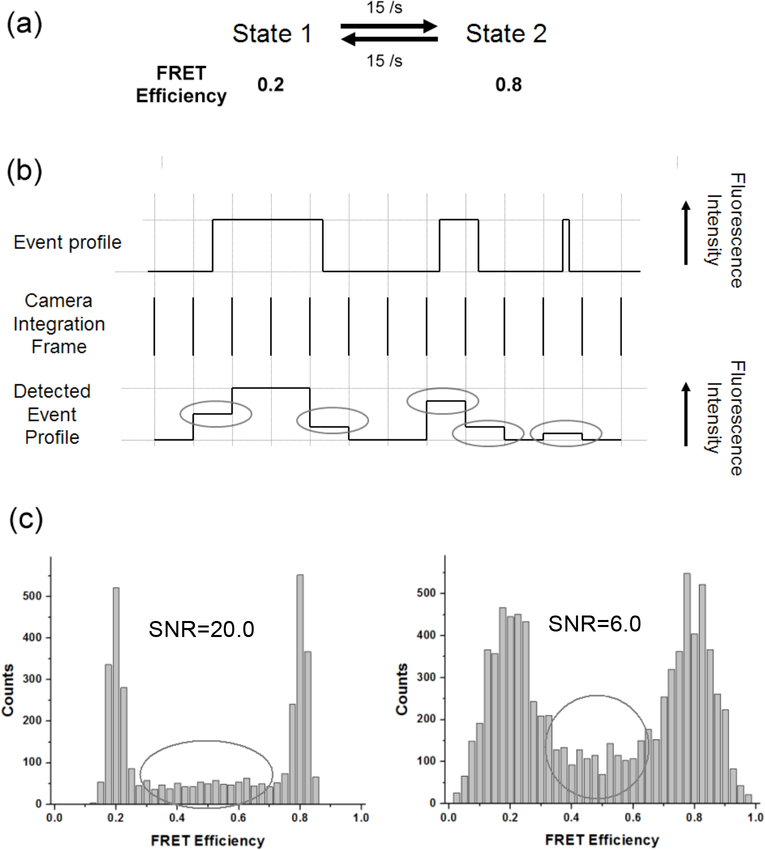
There are fundamental and practical limitations when applying HMM to SM FRET signals. First, longer signal integration time than the event duration yields artifacts in signal ¹⁷, i.e. short lifetime events register lower or higher FRET values than normal that can be seen as either a different state or noise (Fig. 1). Second, the unsynchronized detection to enzyme dynamics also causes artifacts (Fig. 1). The first and the last detection frame of a single FRET event include only a partial frame event because the enzyme dynamics is not synchronized to detection frames. Transitions between two states, therefore, generally leave a small population of FRET events between two FRET peaks (Fig. 1). Short lifetime events elongate the detected lifetime of a FRET state, and unsynchronized detection shortens it. A formula to fit FRET distribution histograms with these artifacts has already been reported ¹⁷ However, the reported formula yields an analytical solution only in the case of a two-state model. Moreover, the solution takes an unfeasibly long time to be employed in an HMM optimization algorithm, where the probability distribution of a state is typically calculated a million times or more to optimize a reasonable amount of experimental data. Lastly, due to the limited photobleaching lifetimes of conventional dyes, SM FRET traces in many experiments are short fragments, each of which contains only a portion of all possible transitions between states. Therefore, individually optimized HMM parameters per individual trace contain partial information. Recently, it was shown that the average of the logarithm of individual transition matrices can represent the universal transition matrix in some cases ¹⁶. For another instance, computer simulations reveal that a Winsorized mean of the lower 70% of transition matrices can approximate the representative universal transition matrix fairly well in some random cases (data not shown). However, all of the averaging methods yield an unknown level of uncertainty due to the empirically determined weights on individual transition matrices. In order to address these three problems, algorithms of HMM with a modified FRET efficiency distribution and a combined probability of multiple observation sequences were implemented.

Fig. 1.

The effect of short lifetime events and the unsynchronized detection on FRET efficiency distribution. (a) Kinetic scheme of the simulated traces. Two sets of SNR (20.0 and 6.0) were simulated. (b) Illustration of real events and detected events showing examples of short lifetime events and the unsynchronized events to the detector time bin. The first and the last detected frame of the first long lifetime event do not have the same fluorescence intensity level as the rest of the frames in the middle. The second event with a lifetime similar to the detection integration time also registers two frames with lower fluorescence level than normal. The third short lifetime event will register a single frame with a lower fluorescence intensity level than normal. The gray ellipses indicate these abnormal low fluorescence intensities resulting from either the unsynchronized detection or short lifetime events. (c) SM FRET histograms from simulated traces with the kinetic scheme in (a). As SNR becomes higher, randomly scattered FRET efficiency counts between the two FRET peaks become evident (counts in gray ellipses). These counts are due to short lifetime events and the unsynchronized detection.

Experimental Methods

HMM model parameter optimization

In order to extract the kinetic scheme from SM FRET traces, HMM parameters were optimized with the given set of FRET traces. Baum-Welch’s iteration algorithm was used to perform the optimization ⁹. A technical problem of underflow in probabilities can be easily fixed with the known rescaling procedure ⁹. Equations 1 and 2 are the re-estimation formulae for the transition matrix a and the initial state π. For emission probabilities b, continuous observation densities were used to avoid any artifacts arising from digitizing FRET traces ⁹. Observation density distributions of SM FRET traces were assumed to be Gaussian, which is widely used in fitting SM FRET histograms ¹⁸. To consider different background fluorescence intensities and slight shifts in FRET efficiencies due to environmental heterogeneity, multiple Gaussian distributions per state were used. The re-estimation formula for the emission probabilities, then, is given as in Eq. 3. For the re-estimation formulae of μ_j and σ_j, one can follow the procedure for the maximum likelihood estimation of multivariate mixture observation as reported ^9,19

$$a_{ij}=\frac{\sum _{t=1}^{T-1}{\xi }_t(i,j)}{\sum _{t=1}^{T-1}{\gamma }_t(i)}$$ (Eq. 1)

$${\pi }_i={\gamma }_1(i)$$ (Eq. 2)

, where T is the number of time points in the trace, $\sum _{t=1}^{T-1}{\xi }_t(i,j)$ is the expected number of transitions from state i to state j, and $\sum _{t=1}^{T-1}{\gamma }_t(i)$ is the expected number of transitions from state i.

$$b_i(O)=\sum _{j=1}^m{c}_j\frac{1}{\sqrt{2\pi {\sigma }_j^2}}\exp (-\frac{{\left(O-{\mu }_j\right)}^2}{2{\sigma }_j{}^2})$$ (Eq. 3)

, where O is the observation, m is the number of Gaussian distributions per state, μ_j is the peak position of j^th Gaussian component of state i, and σ _j is the width of j^th Gaussian distribution of state i. To accommodate the scattered FRET efficiencies between peaks (Fig. 1), one more asymmetric Gaussian distribution is added to Eq. 3. The Gaussian component is approximated to

$$\sum _j\frac{2c_j}{n_j+1}\sum _m\frac{k_m}{k_{\mathit{\text{total}}}}\frac{2}{\sqrt{2\pi }({\sigma }_j+(\frac{|{\mu }_j-{\mu }_m|}{3}))}\left(\exp (-\frac{{(O-{\mu }_j)}^2}{2{{\sigma }_j}^2})\text{or}\exp (-\frac{{(O-{\mu }_j)}^2}{2{(\frac{{\mu }_j-{\mu }_m}{3})}^2})\right)$$ (Eq. 4)

, then that for the main peak is normalized to

$$\sum _j\frac{\left(n_j-1\right)c_j}{n_j+1}\frac{1}{\sqrt{2\pi {\sigma }_j^2}}\exp (-\frac{{\left(O-{\mu }_j\right)}^2}{2{\sigma }_j{}^2})$$ (Eq. 5)

, where k are the rate constants defining rates out of the state j, and n is the biggest integer smaller than the average number of consecutive data points for the state (e.g. average duration of the state in terms of signal frames). The first exponential term in Eq. 4 is applied when O is not related to state m, while the second term is applied when O falls between state j and m. These two equations are valid only when the state lifetime is equal to or longer than the signal integration time. The denominator 3 in the width of the new Gaussian in Eq. 4 is chosen to have negligible probability of one FRET state j beyond the other FRET state m (<0.27%) while there are still significant FRET distribution between the FRET peaks. It is confirmed by HMM optimization that a denominator of 3 works best among 2, 3 and 4 (data not shown). The final formula for b is then as follows.

$$b_i(O)=\sum _j\frac{c_j}{n_j+1}\left[\begin{array}{llll}\sum _m\frac{k_{\mathit{\text{t}}}}{k_{\mathit{\text{total}}}}\frac{4}{\sqrt{2\pi }({\sigma }_j+(\frac{\mid {\mu }_j-{\mu }_m\mid }{3}))}\hfill & (\exp (-\frac{{(O-{\mu }_j)}^2}{2{\sigma }_j{}^2})\hfill & \text{or}\hfill & \exp (-\frac{{(O-{\mu }_j)}^2}{2{(\frac{{\mu }_j-{\mu }_m}{3})}^2}))\hfill \\ +\frac{(n_j-1)}{\sqrt{2\pi {\sigma }_j{}^2}}\exp (-\frac{{(O-{\mu }_j)}^2}{2{\sigma }_j{}^2})\hfill & \hfill & \hfill & \hfill \end{array}\right]$$ (Eq. 6)

A straight line between the FRET peaks convolved with Gaussian distributions is found to yield less accurate results with significantly longer optimization time than the asymmetric Gaussian distribution.

In addition to the above modifications in the FRET efficiency distribution, a single transition matrix and a single set of emission probabilities are used to maximize the total probability of individual P(O\A), i.e. $\prod _{l=1}^n{P}_l\left(O_l\mid \left\{a,b,{\pi }_l\right\}\right)$, instead of optimizing P(O\λ) of individual traces, where l is the index of individual SM FRET traces of which the total number is n. Rabiner’s re-estimation formulae for multiple observation sequences are used with unit weighting instead of P⁻¹ weighting ⁹. It is more logical to use unit weighting for SM FRET data because a mere number of time points in a trace does not necessarily increase the information content of the trace. The number of transitions can better represent the amount of information contained in a trace. Therefore, P⁻¹ weighting in cases where many time points are steady instead of dynamic, as in SM FRET, is inappropriate. One optimization of HMM model parameters generally takes several tens of seconds to several hours depending on the number of Gaussian mixtures and the total length of SM FRET traces, but it rarely exceeds an hour with a practical amount of data and a reasonable number of Gaussian distributions per state (< 5) on a Windows system (Microscoft Corp., USA) with a Pentium 4 processor (Intel Corp., USA) or on a Linux system with a Pentium D processor (Intel Corp., USA). The algorithm is implemented in IDL (ITT Industries, Inc., USA).

SM FRET trace simulations

Monte Carlo simulations were carried out to generate SM FRET traces to evaluate the algorithm. The total photon emission rate from a FRET pair of a donor and an acceptor was varied to adjust the Poissonian noise level. FRET dynamics are independent from the photon emission and detection. Time resolution of photon detection is 1 μs and detector integration time is 25 ms, i.e. the observation frame rate is 40 /s. Photon detection efficiency is assumed to be 100%. Independent system dynamics from the monitoring scheme insures the incorporation of the abnormal FRET values due to the limited detection time resolution (Fig. 1).

Results and Discussion

Comparison between a Gaussian distribution and the modified mixed Gaussian distribution for the HMM optimization

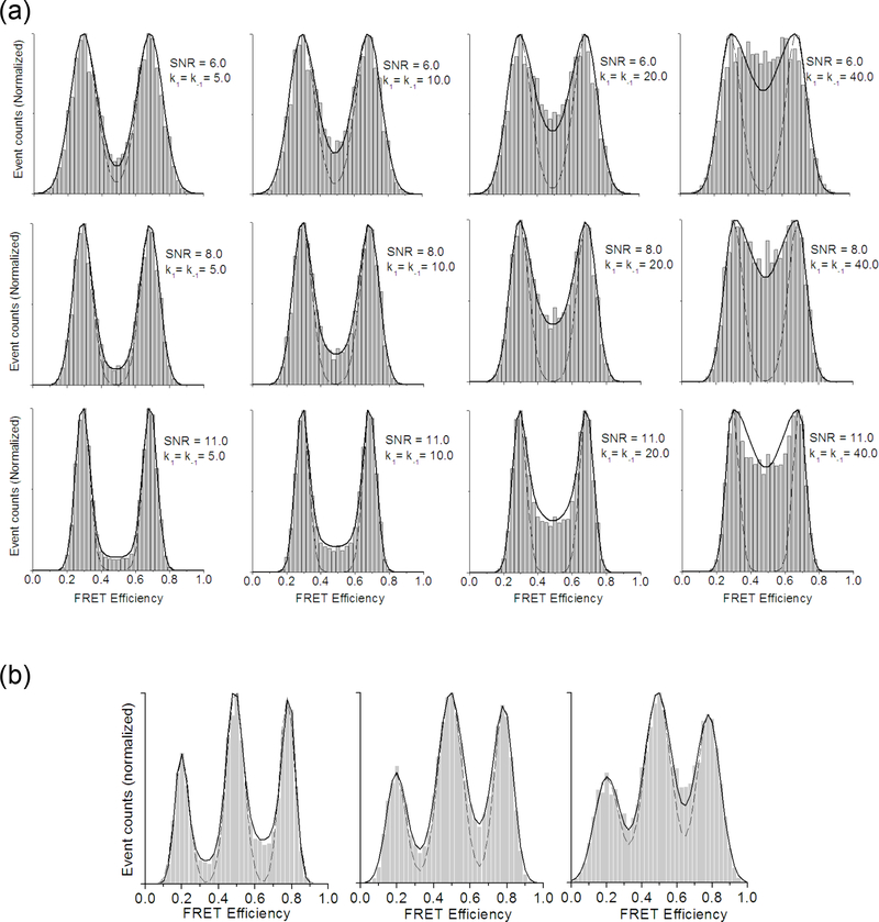
First, the two FRET efficiency distributions (Eq. 3 and Eq. 6) were used to fit histograms from simulated FRET traces (Fig. 2). The histograms were constructed from 100 traces of 500 data points. The fitting parameters are the width and the amplitudes of the FRET peaks. The probability distribution between the Gaussian peaks is well approximated by Eq. 6 as clearly seen in Fig. 2. Although the fitting is not as good as the reported analytical solution ¹⁷, Eq. 6 can be used to fit multiple state models and the computational time is short enough to be employed in an HMM optimization algorithm. It should be noted that as the kinetic rate is higher than half of the observation frame rate, the fitting becomes significantly deviated. Nonetheless, it is clearly shown in Fig. 2 that the modified distribution (Eq. 6) fits the FRET distribution better than Gaussian distributions (Eq. 3).

Fig. 2.

The unmodified (Eq. 3) and modified (Eq. 6) Gaussian distributions as an approximated FRET efficiency distribution. (a) The two distribution functions are used to fit histograms constructed from simulated SM FRET traces with a 2-state model (solid line: fit using Eq. 6, dotted line: fit using Eq. 3). Each panel represents a case of 100 SM FRET traces (500 time points per trace). FRET efficiencies of the two states are 0.3 and 0.7. SNR is controlled by changing photon emission rate. The kinetic rates between the two states are also varied as labeled on each panel. Signal integration time is 25 ms (observation frame rate = 40 /s). SNR range (6.0, 8.0 and 11.0) is chosen to simulate experimental data with reasonable quality attainable in a laboratory. (b) A 3-state model with two different SNR values fit with the two distribution functions (solid line: fit using Eq. 6, dotted line: fit using Eq. 3). Each panel represents a case of 100 SM FRET traces of 500 time points. FRET efficiencies for the three states are 0.2, 0.5, and 0.8. Kinetic rates between the three states are k₁=10.0, k₋₁=5.0, k₂=10.0, k₋₂=12.0. SNR for the left panel is 11.0, 8.0 for the center panel, and 6.0 for the right panel.

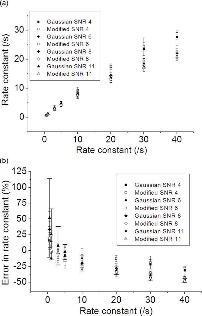
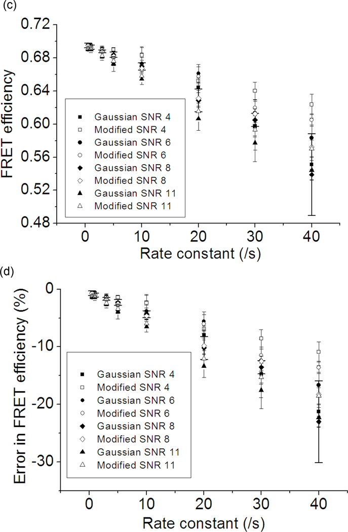
Next, the performance of the two distributions in the HMM optimization is evaluated. The number of states and the kinetic scheme of the system were assumed to be known, i.e. the size of the transition matrix was set constant and some transition matrix elements were set to zero by using a mask matrix. Kinetic rates are the product of the optimized transition matrix and the observation frame rate (= 40 /s). A set of 2500 SM FRET traces were generated per case (varying SNR and kinetic rates) where one trace contains 350 data points. The system switches between 0.3 and 0.7 FRET state, and the rate going from 0.3 to 0.7 state is fixed at 0.5 /s while the rate going from 0.7 to 0.3 state is varied. The optimization is carried out with 175000 data points per case (500 traces per optimization). The plotted results in Fig. 3 are obtained from 5 optimizations per data point. The 175000 points of data were chosen to ensure that the difference in the results is likely due to the difference in the probability distribution functions (the effect of the number of data points on the optimization performance follows in a later section). It is shown in Fig. 3 that the Gaussian distribution (Eq. 3) and the modified Gaussian distribution (Eq. 6) underestimate both the kinetic rate and the FRET efficiency. The most pronounced difference between the two distribution functions is the high uncertainty in the kinetic rates optimized with the unmodified Gaussian distribution in case of high SNR traces. This abnormally high optimization uncertainty is likely due to the fact that as the peaks get narrower (i.e. as the SNR improves and the rate becomes lower), the probability distribution between the FRET peaks according to Eq. 3 becomes effectively zero. The lower uncertainty of the modified distribution (<10% in most of the cases) makes it a better choice for the SM FRET data analysis. It is also clear that FRET efficiency is more accurate when the modified distribution (Eq. 6) is used although the difference becomes smaller as the kinetic rate decreases and SNR becomes more realistic (6~8) because the unmodified Gaussian distribution (Eq. 3) would be accurate enough to model the system under these conditions. The results for the rate 0.5 /s and FRET efficiency 0.3 are omitted because the performance were equally good with Eq. 3 and Eq. 6 within the error of 5% in the kinetic rate and the FRET efficiency.

Fig. 3.

The effect of the rate constant on the HMM optimization performance of the two probability distribution functions (Eq. 3 and Eq. 6). Five sets of 500 simulated traces with 350 time points per trace were optimized to give one data point with an error bar. The system is composed of 2 FRET states with FRET efficiencies of 0.3 and 0.7. The rate going from 0.3 to 0.7 state is fixed at 0.5 /s and the backward rate is varied (0.5, 1.0, 3.0, 5.0, 10.0, 20.0, 30.0, 40.0 /s). Signal integration time is 25 ms (observation frame rate = 40 /s). SNR (i.e. photon emission rate from the fluorophore) was varied in order to examine its effect on the results. A data label starting with “Gaussian” indicates that the optimization is performed with Eq. 3. “Modified” is used if the optimization was performed with Eq. 6. (a) Optimized backward rates plotted against the given rate constants. (b) The error in the optimized backward rate constants plotted against the given rate constants. (c) Optimized FRET efficiency of the 0.7 FRET state plotted against the backward rates. (d) Errors in the optimized FRET efficiency of the 0.7 FRET state plotted against the backward rates.

Effect of number of data points on the performance of the algorithm

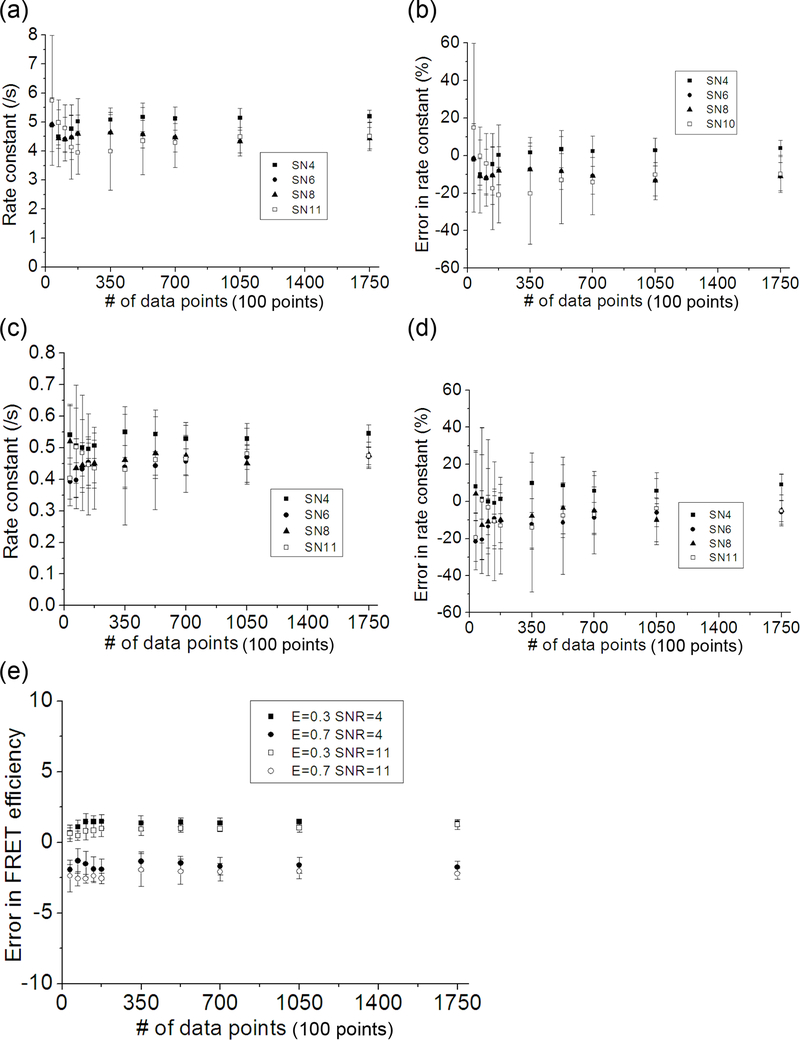
The effect of the number of data points used in the optimization is examined (Fig. 4). A set of FRET traces with FRET efficiencies of 0.3 and 0.7 was simulated. The rate going from 0.3 to 0.7 is 0.5 /s, and the rate going from 0.7 to 0.3 is 5.0 /s. Five optimizations were performed per case. It is shown in Fig. 4 that the 3500 data points which contains 79.5 transitions with the given transition rates are good enough to yield optimization results with <3% error in FRET efficiency and <21% error in the rates on average. As the number of the data points increases, the uncertainty in the rates decreases, but the benefit is not sufficient to compensate for the increase in the number of data points after 7000 data points (159 transitions).

Fig. 4.

The effect of the amount of data on the performance of HMM optimization. The simulation conditions are the same as in Fig. 3 except that the optimization was performed using only the modified distribution function (Eq. 6) and the kinetic rates are fixed at 0.5 /s and 5.0 /s respectively for the forward and the backward rates. The amount of data used in the optimization was varied (10, 20, 30, 40, 50, 100, 150, 200, 300, and 500 traces which are equivalent to 3500, 7000, 10500, 14000, 17500, 35000, 52500, 70000, 105000, and 175000 data points) and the SNR was also varied (4.0, 6.0, 8.0, and 11.0). “SNR” is further abbreviated to “SN” in charts (a)~(d). (a) The optimized backward rates (5.0 /s) plotted against the number of data points used in the optimization. (b) The errors in the optimized backward rates plotted against the number of data points. (c) The optimized forward rates (0.5 /s) plotted against the number of data points used in the optimization. (d) The errors in the forward rates plotted against the number of data points. (e) Errors in the optimized FRET efficiency levels plotted against the number of data points used in the optimization.

Effect of ΔFRET on the performance of the algorithm

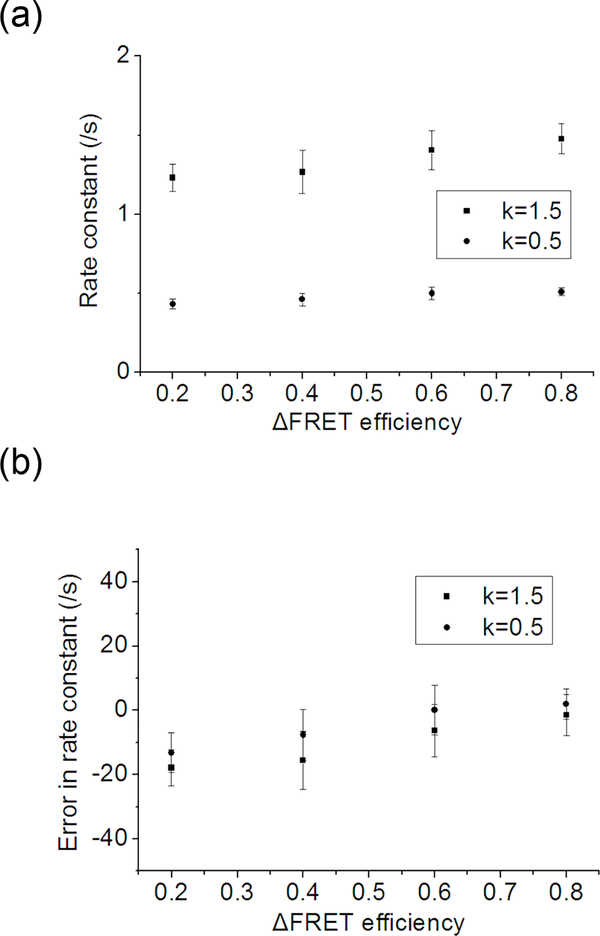
A set of FRET traces with two states of varying FRET efficiencies – (0.1, 0.9), (0.2, 0.8), (0.3, 0.7) and (0.4, 0.6) – was simulated. The rate going from a lower FRET state to a higher FRET state is 0.5/s, and the rate going the other direction is 1.5 /s. The optimization is carried out three times on 7000 total data points per case. Fig. 5 shows errors in the kinetic rates for different ΔFRET cases. It is clearly shown that the optimization yields more accurate results as ΔFRET increases.

Fig. 5.

The effect of ΔFRET efficiency on HMM optimization performance. 1500 SM FRET traces were simulated with SNR of 20.0 and the FRET efficiencies are varied (0.4/0.6, 0.3/0.7, 0.2/0.8, and 0.1/0.9 for the two FRET states to simulate ΔFRET of 0.2, 0.4, 0.6, and 0.8 respectively). Rates between the two states are 0.5/s and 1.5/s. A high SNR and low rates ensure that any difference in the optimization performance can be attributed to the different ΔFRET. (a) Optimized rate constants plotted against the ΔFRET efficiency. (b) Errors in the optimized rate constant plotted against the ΔFRET efficiency.

Performance of the algorithm with multiple states and multiple Gaussian distributions per state

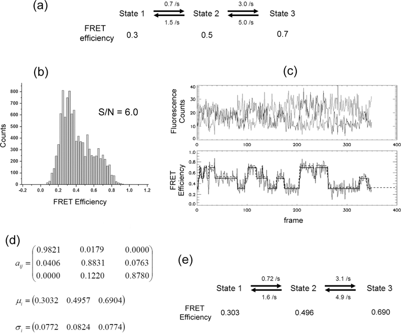
Thirty SM FRET traces with 350 time points each were simulated to evaluate the algorithm in the optimization with multiple states. Traces follow given kinetic scheme and rates as shown in Fig. 6(a). SNR is 6.0 and the noise originates solely from Poissonian photon emission statistics. The amount of data simulated per case is about half of what is typically taken to extract kinetics information (kinetics scheme and kinetic rates) from experiments. Fig. 6(e) shows the optimized kinetic rates and the FRET efficiencies. The highest error in the FRET efficiency is 1.4% for state 3. Errors in the estimated kinetic rates are also low (< 6.7 %). Overall, it is confirmed that the maximization of $\prod _{l=1}^n{P}_l\left(O_l\mid \left\{a,b,{\pi }_l\right\}\right)$ yields the optimum model parameters for a system with multiple FRET states.

Fig. 6.

Demonstration of SM FRET data analysis with the proposed HMM algorithm. (a) Kinetic scheme of the 3-state system simulated. FRET efficiencies for each state are shown below the state label and kinetic rates are also shown in the kinetic scheme. Thirty SM FRET traces with 350 time points each (about a half of the typical amount of experimental data to extract kinetics information) were simulated. Signal integration time is 25 ms (observation frame rate = 40 /s). Photon emission rate of 1440 Hz was used to simulate traces with SNR 6.0. No additional background was added. (b) The histogram of 30 SM FRET traces simulated. (c) An example of simulated SM FRET traces and idealized FRET state transitions by the proposed HMM optimization. The thick gray line in the upper panel is the donor fluorescence count and the thin black line is the acceptor fluorescence count. Noisy signal in the bottom panel is the calculated FRET efficiency (= acceptor fluorescence intensity / (acceptor fluorescence intensity + donor fluorescence intensity)). The solid straight line is the idealized FRET efficiency trace with the optimized HMM model parameters. The dashed straight line is the hidden state trace. The dashed line is shifted slightly upward to clarify the view. (d) The optimized model parameters of HMM. Transition matrix was restricted to the kinetic scheme as shown in (a), i.e. off-diagonal elements were set to zero by using a mask during the optimization. (e) Kinetic rates and FRET efficiencies calculated from the optimized model parameters in (d). Transition matrix elements multiplied by the detection frame rate (= 40 /s) yields the corresponding kinetic rates. μ is the set of FRET efficiencies of each state. σ is the noise in FRET efficiency and is in good agreement with the calculated FRET efficiency noise for each state according to the Beta distribution, which are 0.075, 0.082, and 0.075 for state 1, state 2, and state 3, respectively. The slight discrepancy between the estimated and the given FRET efficiency noise of state 1 or state 3 is likely due to the approximation of the Beta distribution to a Gaussian distribution.

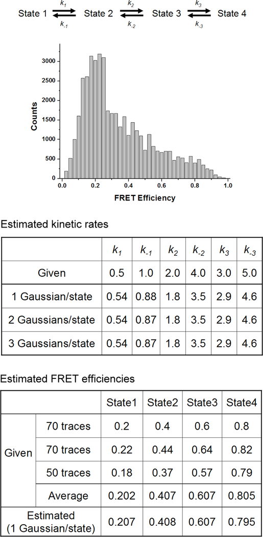
In experiments, the FRET efficiency of a state can vary slightly from trace to trace due to different background fluorescence levels and other environmental heterogeneity that affects the photophysics of fluorescence labels. To examine how this slight variation in FRET efficiency affects the performance of the algorithm, the optimized model parameters with different numbers of Gaussian distributions per state were compared. The model parameters were optimized for FRET traces with 4 states. These FRET traces are composed of three sets of slightly varying FRET efficiencies (Fig. 7). Based on the optimized model parameters, it was revealed that the algorithm does not discriminate slightly varying FRET efficiencies belonging to one state. Instead, it finds the overall average FRET efficiency and standard deviation of the state from all of the FRET traces used in the optimization. Therefore, different background level and other environmental heterogeneity that causes slight shifts in FRET efficiency do not lower the accuracy of the model parameters optimized with single Gaussian distribution per state.

Fig. 7.

The effect of variations in FRET efficiencies due to environmental heterogeneity on the accuracy of the optimized HMM model parameters. A 4-state system was simulated with the same simulation conditions as in Fig. 6 except the kinetic scheme and the number of traces used. Three different sets of traces were simulated with different sets of FRET efficiencies to simulate FRET efficiencies varied by environmental heterogeneity. Shown FRET efficiency histogram is constructed from 190 simulated traces. Among the 190 traces, 70 traces have one set of FRET efficiencies, another set of 70 traces has a different set of FRET efficiencies, and the other 50 traces have another different set of FRET efficiencies as shown in the table of “Estimated FRET efficiencies”. One, two, or three Gaussian distributions per state were used to optimize the HMM model parameters to see the effect of the variations in FRET efficiencies on the accuracy of the parameters. The transition matrix was restricted to the kinetic scheme (i.e. off-diagonal elements were set to zero by using a mask during the optimization). Results in the table of “Estimated kinetic rates” show that one Gaussian distribution per state can optimize the model parameters as well as two or more Gaussian distributions per state.

Deducing the number of states and kinetic scheme

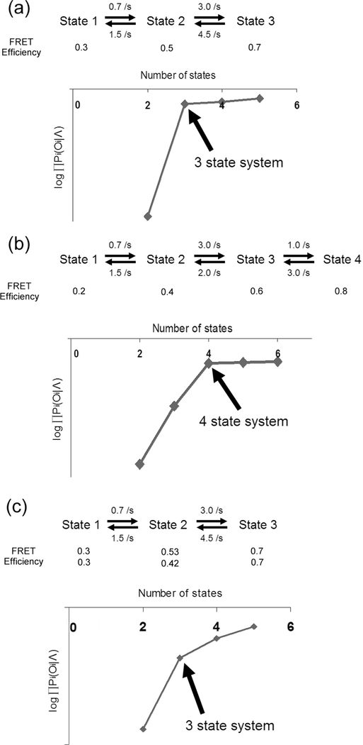
In previous sections, model parameters were optimized with known kinetic scheme and the known number of states. In reality, kinetic schemes and the number of states are normally unknown. To deduce the number of states of a system, one can compare $\prod _{l=1}^n{P}_l\left(O_l\mid \left\{a,b,{\pi }_l\right\}\right)$ optimized with a series of different numbers of states. As the number of states in the optimization increases, $\prod _{l=1}^n{P}_l\left(O_l\mid \left\{a,b,{\pi }_l\right\}\right)$ will always increase following the power law because it is the product of individual probabilities each of which is linearly affected by the increase in the number of states. By plotting $\log [\prod _{l=1}^n{P}_l\left(O_l\mid \left\{a,b,{\pi }_l\right\}\right)]$ with respect to the number of states, it is expected that there will be a distinct point where $\mathrm{\Delta }\log [\prod _{l=1}^n{P}_l\left(O_l\mid \left\{a,b,{\pi }_l\right\}\right)]$ abruptly decreases (Fig. 8). As shown in Fig. 8, the point of abrupt change in $\mathrm{\Delta }\log [\prod _{l=1}^n{P}_l\left(O_l\mid \left\{a,b,{\pi }_l\right\}\right)]$ is the smallest number of states that can model the system and is identified as the number of states of the system. As the noise level of SM FRET traces becomes higher, the residual increase in $\log [\prod _{l=1}^n{P}_l\left(O_l\mid \left\{a,b,{\pi }_l\right\}\right)]$ past the smallest number of states becomes bigger (Fig. 8(c)). Nevertheless, it is straightforward to determine the number of states. Once the right number of states is identified, the kinetic scheme can be easily deduced from the optimized transition matrix. For instance, if there is no direct transition between two states in FRET traces, the corresponding transition matrix element will be unfeasibly small as demonstrated in the next section.

Fig. 8.

Demonstration of deducing the number of hidden states from SM FRET traces. Two 3-state systems and one 4-state system were simulated with the given rates and FRET efficiencies. SNR 6.0 was used (noise solely from Poissonian photon emission statistics). Fifty traces per each were simulated for (a) ~ (c) (350 time points per trace). In (c), two sets of FRET efficiencies (30 and 20 traces) were simulated. Each set of 50 traces were used to optimize the model parameters with 3 ~ 6 states. Each chart in (a) ~ (c) shows $\log [\prod _{l=1}^n{P}_l\left(O_l\mid \left\{a,b,{\pi }_l\right\}\right)]$ plotted against the number of states used in the optimization. In each case of (a) ~ (c), there is a distinct number of state where $\mathrm{\Delta }\log [\prod _{l=1}^n{P}_l\left(O_l\mid \left\{a,b,{\pi }_l\right\}\right)]$ drops abruptly informing the smallest number of required states to model the observation sequence. These points are indicated with arrows. In a noisier data set (c), $\mathrm{\Delta }\log [\prod _{l=1}^n{P}_l\left(O_l\mid \left\{a,b,{\pi }_l\right\}\right)]$ change is not as abrupt as in cases (a) and (b). Nevertheless, it is straightforward enough to identify the number of states in (c). In charts, $\prod _{l=1}^n{P}_l\left(O_l\mid \left\{a,b,{\pi }_l\right\}\right)$ is abbreviated to $\prod P_i\left(O_i\mid \Lambda \right)$.

Demonstration of extracting kinetics information from SM FRET traces

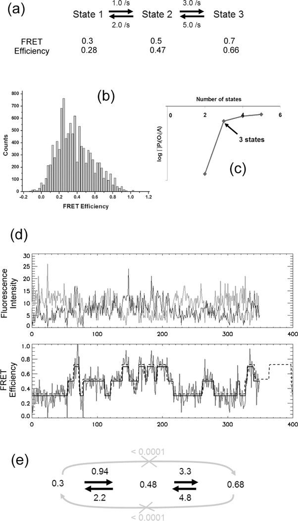
Based on the procedure described above, a process of extracting kinetic information from SM FRET traces is demonstrated in Fig. 9. A very noisy set of data (SNR calculated from Poissonian photon emission statistics = 4.0) from a three-state system was simulated. Two sets of FRET efficiencies were used to simulate two different sets of data taken in two different environments. First, the maximum $\prod _{l=1}^n{P}_l\left(O_l\mid \left\{a,b,{\pi }_l\right\}\right)$ is calculated with the optimized model parameters with 2, 3, 4, and 5 states and a single Gaussian distribution per state. As shown in Fig. 9(c), it is clear that the system dwells on three states. An example of idealized FRET traces from optimum model parameters with three states is shown in Fig. 9(d). From the simulation, it was found that state 1 and state 3 are not connected to each other since the transition matrix elements are too small (< 0.0001 /s) to be real – i.e. based on the length of the longest trace (= 8.75 sec), the slowest possible transition rates between states should not be much lower than 1/8.75 = 0.11 /s. Estimated kinetic rates are in good agreement with the given rates within 10% error.

Fig. 9.

Demonstration of extracting kinetics information from SM FRET traces. A set of 30 SM FRET traces (350 time points each) with SNR 4.0 (noise solely from Poissonian photon emission statistics) was simulated and used to optimize the model parameters of HMM. SNR is set to be worse than a typical experimental SNR in order to test the robustness of the algorithm. (a) Kinetic scheme used in the simulation. (b) FRET Efficiency histogram of the simulated traces.(c) $\log \prod _{l=1}^n{P}_l\left(O_l\mid \left\{a,b,{\pi }_l\right\}\right)$ vs. the number of states indicating that the system dwells on 3 states.(d) An example of SM FRET traces (upper panel: the gray line is the donor fluorescence intensity and the black line is the acceptor fluorescence intensity), FRET efficiency (the noisy signal in the lower panel), and the idealized FRET efficiency sequence (the solid line over the noisy FRET signal in the lower panel) by the algorithm with 3 states. The dashed line in the lower panel is the given event sequence shifted slightly upward to clarify the view. (e) Reconstructed kinetic scheme from the optimized transition matrix. Gray lines show null transitions found by the algorithm as explained in the text.

Conclusions

Using HMM, a systematic way of extracting kinetics information from noisy SM FRET data is demonstrated. There are three distinct sources of noise in SM FRET signal: i) Poissonian noise from photon emission statistics, ii) noise from environment such as background fluorescence, stray light, and noise in detection devices, and iii) short lifetime events and the unsynchronized detection. It is demonstrated that the errors from the first two sources can be suppressed by using the proposed algorithm. The third source of noise, however, is unavoidable although HMM with the proposed modified FRET distribution can reduce the error. Nevertheless, thanks to the reasonably high precision of the proposed method, HMM optimization results can be used to report the kinetic rates of an SM FRET system when the report accompanies the information on the level of error due to the limited detection time resolution.

References

- (1).Ha T; Enderle T; Ogletree DF; Chemla DS; Selvin PR; Weiss S Proc. Natl. Acad. Sci. U.S.A. 1996, 93, 6264. [DOI] [PMC free article] [PubMed] [Google Scholar]
- (2).Weiss S Nature Struct. Biol. 2000, 7, 724. [DOI] [PubMed] [Google Scholar]
- (3).McKinney SA; Declais A-C; Lilley DMJ; Ha T Nature Struct. Mol. Biol. 2003, 10, 93. [DOI] [PubMed] [Google Scholar]
- (4).Ha T; Zhuang X; Kim HD; Orr JW; Williamson JR; Chu S Proc. Natl. Acad. Sci. U.S.A. 1999, 96, 9077. [DOI] [PMC free article] [PubMed] [Google Scholar]
- (5).Zhuang X; Bartley LE; Babcock HP; Russell R; Ha T; Herschlag D; Chu S Science 2000, 288, 2048. [DOI] [PubMed] [Google Scholar]
- (6).Ha T; Rasnik I; Cheng W; Babcock HP; Gauss GH; Lohman TM; Chu S Nature 2002, 419, 638. [DOI] [PubMed] [Google Scholar]
- (7).Myong S; Rasnik I; Joo C; Lohman TM; Ha T Nature 2005, 437, 1321. [DOI] [PubMed] [Google Scholar]
- (8).Lee T-H; Blanchard SC; Kim HD; Puglisi JD; Chu S Proc. Natl. Acad. Sci. U.S.A. 2007, 104, 13661. [DOI] [PMC free article] [PubMed] [Google Scholar]
- (9).Rabiner LR Proc. IEEE 1989, 77, 257. [Google Scholar]
- (10).Baum LE; Petrie T Ann. Math. Stat. 1966, 37, 1554. [Google Scholar]
- (11).Viterbi AJ IEEE trans. inform. theory 1967, IT-13, 260. [Google Scholar]
- (12).Forney GD Proc. IEEE 1973, 61, 268. [Google Scholar]
- (13).Qin F; Auerbach A; Sachs F Biophys. J. 2000, 79, 1928. [DOI] [PMC free article] [PubMed] [Google Scholar]
- (14).Qin F; Auerbach A; Sachs F Biophys. J. 2000, 79, 1915. [DOI] [PMC free article] [PubMed] [Google Scholar]
- (15).Smith DA; Steffen W; Simmons RM; Sleep J Biophys. J. 2001, 81, 2795. [DOI] [PMC free article] [PubMed] [Google Scholar]
- (16).McKinney SA; Joo C; Ha T. Biophys. J. 2006, 91, 1941. [DOI] [PMC free article] [PubMed] [Google Scholar]
- (17).Gopich IV; Szabo A J. Phys. Chem. B 2007, 111, 12925. [DOI] [PubMed] [Google Scholar]
- (18).Dahan M; Deniz AA; Ha TJ; Chemla DS; Schultz PG; Weiss S Chem. phys. 1999, 247, 85. [DOI] [PMC free article] [PubMed] [Google Scholar]
- (19).Baum LE; Petrie T; Soules G; Weiss N Ann. math. stat. 1970, 41, 164. [Google Scholar]