Structural covariance networks in schizophrenia: A systematic review Part II

Abstract

Background:

Examination of structural covariance network (SCN) is gaining prominence among the strategies to delineate dysconnectivity that case-control morphometric comparisons cannot address. Part II of this review extends on the part I of the review that included SCN studies using statistical approaches by examining SCN studies applying graph theoretic approaches to elucidate network properties in schizophrenia. This review also includes SCN studies using graph theoretic or statistical approaches on persons at-risk for schizophrenia.

Methods:

A systematic literature search was conducted for peer-reviewed publications using different keywords and keyword combinations for schizophrenia and risk for schizophrenia. Thirteen studies on schizophrenia and five on persons at risk for schizophrenia met the criteria.

Results:

A variety of findings from over the last 1½ decades showing qualitative and quantitative differences in the global and local structural connectome in schizophrenia are described. These observations include altered hub patterns, disrupted network topology and hierarchical organization of the brain, and impaired connections that may be localized to default mode, executive control, and dorsal attention networks. Some of these connectomic alterations were observed in persons at-risk for schizophrenia before schizophrenia onset.

Conclusions:

Observed disruptions may reduce network efficiency and capacity to integrate information. Further, global connectomic changes were not schizophrenia-specific but local network changes were. Existing studies have used different atlases for brain parcellation, examined different morphometric features, and patients at different stages of illness making it difficult to conduct metanalysis. Future studies should harmonize such methodological differences to facilitate metanalysis and also elucidate causal underpinnings of dysconnectivity.

1. INTRODUCTION

Investigating the complex organization of the brain can help better improve understand the pathophysiology of schizophrenia. Both within-subject and between-subject shared brain regional variations that are captured by structural covariance networks (SCNs) have been reported for decades. SCNs analyzed using statistical approaches have highlighted shared variational patterns in schizophrenia compared to healthy controls (HC) (reviewed in Part I). Application of mathematical methods, such as graph theoretic approaches to network analysis further enrich these findings by identifying several qualitative and quantitative graph properties at the global, regional, and nodal levels that provide summary measures of complex covariance patterns. Such graph features can be biologically meaningful. This review focuses on studies that used graph theoretic approaches to examine SCNs and the implications of their findings for understanding the pathophysiology and risk for schizophrenia.

2. METHODS

We searched the PubMed, PsychInfo and Embase databases using different keywords for peer-reviewed papers published until July 04, 2021, yielding a number of papers: “structural covariance” (n=11,159), “structural covariance network” (n=1274) and “structural covariance network AND schizophrenia” (n=80), “structural covariance AND schizophrenia” (n=316), “morphometric covariance” (n=495), “morphometric covariance AND schizophrenia” (n=26), “structural covariance network AND graph theory” (n=89), “source based morphometry” (n=262), “source based morphometry AND schizophrenia” (n=33), “structural covariance network AND schizophrenia AND graph theory” (n=9), “high risk schizophrenia” (n=6457), “high risk schizophrenia AND structural covariance” (n=23), “ultra-high risk schizophrenia AND structural covariance” (n=6 papers), “at risk mental state schizophrenia AND structural covariance” (n=13 papers). Manuscripts that met the following criteria were selected: (a) should be published in a peer-reviewed journal, (b) should have examined schizophrenia or risk for schizophrenia using structural MRI, (c) should have well-described image acquisition, processing, statistical and/or mathematical procedures, (d) should have used graph theoretical or other mathematical approaches as the primary method of network analysis, and (e) should compare with appropriate HC.

3. RESULTS

Application of graph theoretic approaches to the investigation of structural covariance in schizophrenia started in the latter part of the 2000s. Of the 129 total publications, 13 were identified that used mathematical approaches to examine schizophrenia SCN and 5 studies that examined persons at-risk for schizophrenia (statistical methods, n=3; graph theory, n=2) were selected to discuss here (Fig 1).

Figure 1:

PRISMA diagram showing selection of studies for review

An introduction to key concepts in graph theory can be found in short books (Gould, 2012). A brief introduction to the graph theory concepts is provided here to help understand the key findings of the published manuscripts.

3.1. A PRIMER ON GRAPH THEORY

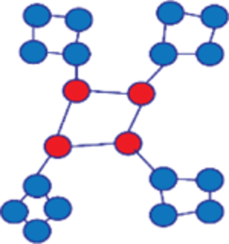
A graph is a collection of nodes or vertices and connections among them, called edges (Fig 2). In the SCNs, the nodes correspond to regions-of-interests (ROIs) and the edges are pairwise correlations of morphometric measures of these ROIs. Edges can be endowed with weights based on correlation strengths between the connected nodes resulting in weighted networks. These strengths can be thresholded to produce a binary graph where above-threshold edges are given values of 1 and below-threshold edges are given values of 0. In graph visualizations, weights are represented by edge thickness, while the node sizes are scaled to reflect their strengths or densities. Graphs are directed when a directionality of correlations (based on some causality measure) is included (represented by edges with arrows) or undirected when no directionality is represented. Graph features that reflect patterns of correlations globally, regionally or locally can be computed mathematically; such quantities include measures of integration (characteristic pathlength, global efficiency), segregation (clustering coefficient, transitivity, modularity), resilience (degree distribution) and centrality (closeness centrality, betweenness centrality) (Rubinov and Sporns, 2010). Table 1 gives an overview of selected graph measures along with mathematical explanations (Newman, 2018). For simplicity, we discussed these measures for undirected graphs.

Figure 2:

A schematic of a graph consisting of 18 nodes (V1 - V18) and edges that connect the nodes. Edges are weighted (indicated by the thickness of the edges such that thicker edges indicate higher correlations). Number of edges associated with a node is the degree, e.g., nodes V6 and V12 have a degree of 3 while V5 has degree 5. Orange boxes include modules or communities within the graph where the nodes within the communities are more densely interconnected compared to the nodes outside of the communities.

Table 1:

Some important graph measures that can be obtained using graph theory from the covariance matrices along with their definitions and mathematical description.

Graph measure		Global/local	Type of measure	Definition and a brief description	Mathematical formula
Degree		Local	Centrality	Number of edges a node is associated with, e.g., the green node has a degree of 5 while blue nodes have a degree of 1. When every node has the same degree, such a graph is called a regular graph.	Maximum degree, ∆(G) = max{deg(v)|v ∈ V(G)} Minimum degree, ∂(G) = min{deg(v)|v ∈ V(G)} where G is the graph and V(G) is the set of nodes or vertices in the graph.
Density		Global	Integration	Density is the average of normalized degrees of all nodes. The number of edges in a network is normalized by the size of the network. As more edges are added to a graph, the densities of at least some nodes grow. In the example when the dashed edges are included along with the solid ones, the graph becomes complete, and the density goes to 1.	$D=\frac{2{\sum }_{x,y}{A}_{x,y}}{N\left(N-1\right)},x>y$ where A is the adjacency matrix and N is the number of nodes in the graph.
Strength		Local	Centrality	The sum of all edge weights connecting to a node. For example, in a network with 5 nodes with edge weights for the green node given by 0.5, 0.75, 0.6 and 0.4, then the strength of that node is 2.25.	$S_x=\sum _y{A}_{x,y},x\ne y$ Nodal strength of node x is defined as the sum of weights of edges between x and y, where y is all other nodes in the network.
Eigenvector centrality		Global	Centrality	A measure of the influence of a node on the network computed by determining the extent to which a node connects to high degree nodes. In the example, the green node is connected to the two highest-degree nodes in the graph (nodes of degree 3 and 4) and hence has the highest eigenvector centrality of all nodes in the graph.	$C_E\left(x\right)=\frac{1}{\lambda }\sum _{y\in M\left(x\right)}{C}_E\left(y\right)=\frac{1}{\lambda }\sum _{y\in V\left(G\right)}{A}_{x,y}{C}_E\left(y\right)$ where λ is the largest eigenvalue of the adjacency matrix A (guaranteed to be positive as long as there are paths between all pairs of nodes), M(x) is a set of neighbors to vertex x, and V is the set of all vertices in the graph G. Depending on whether x and y are neighbors, Ax,y takes a value or 0 or 1.
Betweenness centrality		Can be calculated both at the global or local levels	Centrality	A number between 0 and 1 corresponding to the fraction of shortest paths between pairs of nodes that pass through a node. In the graph shown, every pair of blue nodes is connected by exactly one shortest path of length 2, which passes through the green node and no others, so the green node has a high betweenness centrality and all blue nodes have betweenness centrality equal to 0.	$C_B\left(x\right)=\sum _{u\ne v\ne x}\frac{{\sigma }_{uv}\left(x\right)}{{\sigma }_{uv}}$ where u and v range over all of the pairs of distinct vertices, also distinct from x, in the graph, σuvis the number of shortest paths between u and v, and σuv(x) is the number of these paths that pass through x.
Closeness centrality		Can be calculated both at the global or local levels	Centrality	Average length of the shortest paths between the nodes and all other nodes. For the green node, the closeness centrality is 5/(1+1+1+1+2) = 5/6.	$C\left(x\right)=\frac{N-1}{{\sum }_{y}d\left(y,x\right)}$ where N is the number of nodes, d(y, x) is the distance (shortest pathlength) between vertices x and y.
Hub		Global	Centrality	Degree, eigenvector, betweenness, and closeness centrality measures can be used to find network hubs. If one of these graph measures for a single node is >2 SD above the average of that graph measure for the network, that node would be a hub. If examining over a threshold range, a hub must be identified in ≥50% of the networks in the range. When a node is defined as a hub, it is considered important to the network and its function. Because the hubs are highly connected (high degree) and are central to the network, without these hubs the network could disintegrate or reroute many connections.	Mi > mean(M) + 2std(M) where M is a centrality measure, i is the node number, and the mean and standard deviation (std) are computed over the values of the measure on all nodes in the network.
Clustering coefficient (CC)		Can be calculated both at the global or local levels	Integration	A measure of how close a node’s neighbors are to forming a complete graph (clique), representing how well connected the neighborhood of a node is. CC quantifies the degree to which connected nodes share neighbors. Global CC can be measured as a ratio of the number of fully connected triplets of nodes (closed triplets) to the total number of triplets, which includes both closed and open (incompletely connected) triplets. The local CC can also be considered as a measure of how close the neighbors of a node come to forming a clique.	$C_i=\frac{2\left|\left\{a_{y,z}:y,z\in N_x,a_{y,z}\ne 0\right\}\right|}{k_x\left(k_x-1\right)}$ where Nx are the neighbors of node x (nodes connected to x), and kx is the number of neighbors. Bars in numerator represent cardinality. For nodes y and z in Nx, the numerator tallies the number of y and z pairs that are also connected.
Characteristic path length (λ)		Global	Integration	Average of the number of edges appearing in the shortest paths linking pairs of nodes in the graph, where “shortest” refers to the fewest edges traversed not to a physical distance between nodes. In many networks, shorter path lengths tend to exist between the nodes that are physically proximal, which would allow for a reduced cost of communication in information-transfer networks. In the example shown, this holds, but if the green edges were removed, then it would no longer be the case, because the green nodes would be physically close but with a relatively long shortest connection path (length 4). λ is considered an efficiency measure in information transfer networks	$\text{λ}=L=\frac{1}{n\left(n-1\right)}\cdot \sum _{x\ne y}d\left(x,y\right)$ where n is the number of nodes in the graph, x and y are nodes, and d is the shortest distance (in terms of number of edges involved) between nodes x and y.
Small worldness (σ)		Global	Integration	The ratio of a graph’s clustering coefficient to that of a degree-matched random graph, divided by the ratio of a graph’s path length divided by that of a degree-matched random graph. If σ≥1, then that network can be defined as a small-world network (Humphries and Gurney, 2008). Path length and CC together determine the small worldness (Watts and Strogatz, 1998). Small world networks feature high levels of clustering and short pathlengths.	$\sigma =\frac{C/C_R}{L/L_R}$ where C is the network CC, CR is average CC calculated from multiple random graphs, L is the characteristic pathlength of the network and LR is the average characteristic pathlength of the random graphs.
Efficiency		Global	Integration	The reciprocal of the characteristic path length (λ). Networks with higher efficiency have lower average pathlength.	E = 1/λ where λ is the characteristic path length.
Modularity		Global	Segregation	Once a network has been partitioned into disjoint groupings of nodes or communities, modularity measures the fraction of edges that connect nodes in the same community, relative to the same fraction produced under random conditions. Higher modularity indicates that a network is strongly segregated into communities, as in the example shown.	$Q=\frac{1}{2m}\sum _{x,y}\left[A_{x,y}-\frac{k_x\cdot k_y}{2m}\right]\frac{S_x{S}_y+1}{2}$ where m is the number of edges in the graph, s is the community membership variable (such that Sx = 1 if x belongs to community 1 and Sx = −1 if x belongs to community 2), A is the adjacency matrix, and kx is the degree of node x. Note that this formula only allows for two communities but can be applied recursively to communities within a larger community.
Assortativity/Disassortativity	Disassortativity on the left and assortativity on the right	Global	Segregation	The correlation coefficient of degree between pairs of connected nodes in a network. When nodes tend to connect to nodes of similar degree a network will have higher assortativity; disassortative networks have negative assortativity values, indicating that nodes tend to connect to nodes with dissimilar degree.	$r=\frac{{\sum }_{ij}\left(A_{ij}-k_i{k}_j/2m\right)k_i{k}_j}{{\sum }_{ij}\left(k_i{\partial }_{ij}-k_i{k}_j/2m\right)k_i{k}_j}$ where ki is degree of node i, kj is degree of node j, kikj/2m is the probability of an edge present between nodes i and j in a random edge environment, ∂ij is the Kronecker delta, and the term Aij ensures that the edges are actually present and the terms for nodes that are neighbors of i contribute to the sum.

There are important differences among degree, density, and strength. While degree is a count of the number of edges to a node, density is degree normalized to the network size, and strength is an arithmetic mean of the weights of edges to a node. Further, the network may segregate into modules of fully connected nodes or into communities with higher within-community correlations and lower correlation with nodes outside the community. Modularity is a measure of the extent to which a network segregates into modules, relative to that expected by chance. Community detection and modularity analysis are two of the most active areas of networks research. While modularity gives a global view of the network, communities provide more nuanced information about how the nodes interact and may function together. For example, communities may correspond to auditory, sensorimotor, executive, and visual domains (Chen et al., 2008).

Centrality of nodes in the graph identifies potentially important nodes by representing some measure of the overall amount of information flow through each node or the extent to which efficient paths pass through each node. Centrality measures such as degree centrality, closeness centrality, betweenness centrality, and eigenvalue centrality, focus on the importance of a node. Other centrality metrics, such as game-theoretic centrality measures the functioning of important nodes as groups, and percolation centrality depends on the state of a node. Thus, percolation centrality of a node could shift depending on that node’s state, such as functional status.

Networks are considered “small world” when the nodes that are not neighbors are connected by short paths. Small-worldness refers to networks that are “highly clustered, like regular lattices, yet have small characteristic pathlengths like random graphs” (Watts and Strogatz, 1998) (Fig 3). The small world index (σ) is calculated using the clustering coefficient (CC) and characteristic pathlength (λ) of the examined network and comparing them to random networks (Table 1). CC measures the local “cliquishness”, which may relate to local sharing of information in a network (Watts and Strogatz, 1998). Similarly, λ quantifies a network’s ability for parallel information propagation (the reciprocal of λ is efficiency). Thus, the small-world topology supports both specialized and distributed information processing making it an attractive model to consider when analyzing anatomical and functional networks. A small world network’s resilience to a pathological attack can be computed by removing one or more nodes from the network along with its corresponding edges and then recalculating the small-world index. The removal of a node and its edges will eliminate certain paths and hence will generally increase the average pathlength. If a node is involved in many short paths, then its removal will have a disproportionately large negative effect on network performance (Bassett and Bullmore, 2006; Bassett and Bullmore, 2017). Thus, resilience is the ability of a network to withstand and/or adapt in the face of “attacks” on the network.

Figure 3:

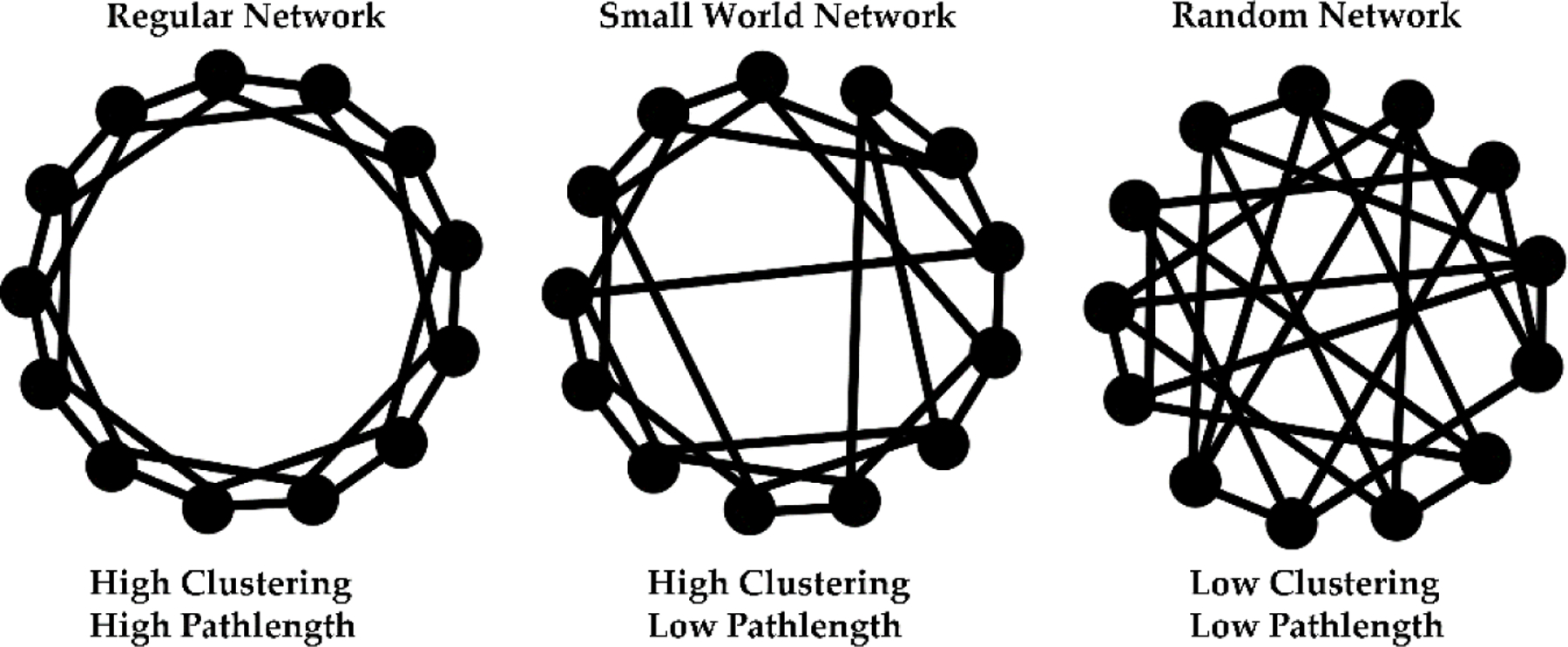
Random graphs, small world network and regular network

This observation engenders the concept of a “hub,” which is sometimes defined as a node having a higher-than-average number of edges and at other times defined as a node belonging to many shortest paths linking nodes anywhere in the graph. These perspectives are related, such that highly connected regions usually have at least some nodes with high centrality. Small world networks tend to include hubs, since the presence of hubs can decrease pathlengths without significantly compromising clustering. Since hubs can be “conduits” for information flow across different parts of the network, hub distribution can potentially influence the network topology and resilience. For example, the presence of multiple hubs distributed across the network can make the network more resilient to pathology (“attack”) by redistribution of connectivity, as opposed to the presence of one or a few mega hubs with very high centrality. Pathological or neuroplastic changes in mega hubs can affect a wide swath of nodes and disrupt the network.

Hubs may be connected to each other and with other densely connected nodes within the network if the network is assortative. Assortativity is the preference of a node to be connected to similar nodes (e.g., nodes of the same/similar degree). Disassortativity is the nodal preference to connect to dissimilar nodes. Thus, a disassortative network would typically have multiple unconnected hubs. Usually biological networks, e.g., gene networks, can be disassortative whereas non-biological networks, e.g., social networks, are assortative. Finding hubs and their locations can help elucidate organizing principles of a network and highlight group differences.

The hubs can be calculated using one or more graph centrality measures: degree, betweenness centrality, closeness centrality, and eigenvalue centrality. A node with any of the centrality measures ≥2 SD above the average across all nodes may be considered a hub (Bassett et al., 2008). Others approaches compare the network to random graphs (Fig 3) and define a hub as any node with a centrality measure ≥1 SD of the corresponding functional data analysis-based curve function (Palaniyappan et al., 2019; Ramsay and Dalzell, 1991), or a node with 1.5 times higher normalized betweenness centrality than the average betweenness of the network (He et al., 2008). Since hubs can change with varying threshold values, when the same hubs are found in over half of the networks over the “small-world regime” or the relative range of threshold values, the hubs are considered significant (Zhang et al., 2012).

Examination of SCN using Graph Theory:

First, structural MRI data from each subject is parcellated into cortical regions using standard atlases. Next, regional morphometric values are calculated for each subject. Following this, a matrix is created to store each subject’s observations in a row and values for each ROI in a column (Step A). An SCN is created for the population, where nodes are defined as column indices of the table (ROIs) and edge weights between nodes are defined as the correlation coefficient between appropriate columns (subject-wise morphometric correlations) (Step B). SCNs can then be analyzed using toolboxes such as the Brain Connectivity Toolbox (Rubinov and Sporns, 2010), the Graph Analysis Toolbox (Hosseini et al., 2012), and NetworkX (https://networkx.org/) (Fig 4).

Figure 4:

A simple schema of an SCN data processing stream

3.2. STUDIES USING GRAPH THEORETIC APPROACHES

3.2.1. Studies Examining Gray Matter (GM) Volume

Five studies examined chronic schizophrenia patients and reported reduced hierarchical network structure and greater mean connectional distance of the network consisting of multimodal but not unimodal or transmodal regions (Table 2) (Bassett et al., 2008), greater global connectivity but sparser local connectivity and less resilient schizophrenia connectome (Palaniyappan et al., 2019), greater brain age gap (Kuo et al., 2020), stronger covariance in first-episode and chronic patients (Zugman et al., 2015), and lack of significant association of SCN strength with gene expression (Liu et al., 2019). Given that each study had unique goals, their main findings were also different. However, all these studies found that the SCNs of chronic schizophrenia patients showed distinctly different global and local covariation patterns compared to HC.

Table 2:

Structural covariance network studies on schizophrenia and related psychotic disorders that applied graph theoretic methods

Author	Sample size and goals of the study	Field strength/Acquisition scheme/Atlas used/Analysis software used	Methods	Main findings
Studies examining gray matter volume SCNs
Bassett et al. (2008)	203 chronic SZ patients and 259 HC. To identify commonalities and differences in network organization of the principal cortical divisions, namely unimodal, multimodal and transmodal (connectivity between unimodal and multimodal networks) cortices(connectivity between unimodal and multimodal networks) networks based on definitions by Mesulam (1998). Second goal was to assess whether these divisions are impacted by SZ.	T1-weighted MRI data from a 1.5 Tesla GE Signa scanner at 1.5 mm thick slices. SPM2 was used to preprocess the scans. Pick Atlas-defined 104 brain regions corresponding to the Brodmann areas + amygdala, hippocampus, striatum, and thalamus were grouped into 28 unimodal, 32 multimodal and 42 transmodal regions.	Partial correlation networks were constructed from residuals of brain regional volumes after regressing out age, sex, and total gray volumes. Fully connected networks over a pre-calculated small-worldness threshold range were examined. Networks examined at global, divisional, and regional scales. Network measures were averaged over the small worldness threshold range for the divisional and regional networks. Compared graph metrics with random networks.	Both HC and SZ networks showed degree distribution that followed exponential truncated power law, and fully connected networks within the cost range. HC showed hierarchical organization in the multimodal network only. Transmodal network was the only cortex that showed significant assortativity. Connection distance was the smallest for the transmodal, intermediate for the unimodal and greatest for the multimodal networks among HC. The right premotor cortex, orbitofrontal cortex, middle temporal cortex, retrosplenial, bilateral DLPFC, and insula were identified as hubs of the HC network by two of the four (degree or centrality) parameters considered. SZ patients showed qualitatively different hubs in the bilateral insula, right inferior temporal cortex, left premotor area, left temporopolar region, left pars opercularis, and right thalamus. less hierarchical multimodal network throughout the small world regime, and greater mean connectional distance of multimodal network compared to HC. No significant differences in in hierarchy, assortativity and connection distance in the unimodal and transmodal cortices. Clustering coefficient was different in 23 nodes at the regional level between SZ and HC.
Zugman et al. (2015)	Examined 143 chronic SZ, 32 first episode SZ and 82 HC. Examined a proposed paradox where structural disconnection may lead to reduced structural covariance whereas reduced volume due to the disease may result in increased covariance	1.5 Tesla Siemens scanner data on structural MRI with 1 mm slice thickness examined. GM volumes of DKT atlas based parcellations for 68 regions was used for SCN.	Integrity-closeness (absolute values of the correlation coefficient between two nodes) and connectivity-closeness (inverse of the absolute values of correlation coefficients between two nodes) were estimated for the groups	Integrity-closeness and connectivity closeness were negatively correlated as expected by their definitions. No significant difference in connectivity-closeness between groups Reduced integrity-closeness in pars orbitalis and insula in SZ compared to HC. Higher degree nodes in patients compared to controls. First episode cases did not differ from chronic schizophrenia.
Liu et al. (2019)	95 chronic SZ patients and 95 HC To identify voxel-level GM volume SCN differences between SZ and HC Whether these differences were related to SZ risk genes (not discussed in this review)	MRI data acquired at 3 Tesla GE scanner with a slice thickness of 1 mm. A GM mask of 32,164 voxels created with the removal of subcortical and cerebellar AAL regions removed. Software used for graph theoretic analysis not stated.	Voxelwise SCN was built using Pearson correlation tests after regressing out the effects of age, sex and ICV using linear regression. Structural covariance/connectivity strength for each voxel was calculated by the weighted sum of correlations r>0.2 with other voxels. Permutation test was used to compare the group level SCS False discovery rate correction was applied for multiple test correction	Degree centrality was the main measure used and structural hubs were also examined. Spatial distribution of high SCS was similar in both groups observed in the medial PFC, posterior cingulate cortex/cuneus, insula, and lateral PFC and temporal regions. SZ showed Increased structural covariance strength in the right orbital part of superior frontal gyrus and bilateral middle frontal gyrus and decreased SCS in the bilateral superior temporal gyrus and the precuneus. Validation with weighted network at raw resolution (1.5×1.5×1.5 mm3), weighted network with r=0.1 and r=0.3 and binarized network at a resolution of 3×3×3 mm3 did not alter the findings None of the genes survived multiple test corrections. A trend was noted for altered pattern of SCS correlation with expression of gene classes involved in therapeutic target and neurodevelopment
Palaniyappan et al. (2019)	41 chronic SZ and 40 HC The goal was to identify if the observed pattern of GM volume loss conforms to coordinated pattern of structural reorganization	MPRAGE data at 1 mm slice thickness acquired; field strength not provided. AAL-90 atlas for parcellation of regions. Graph theoretical approach using Graph Analysis Toolbox, a MATLAB package that integrates with the Brain Connectivity Toolbox.	Group level Pearson correlation matrix of residuals of volumes weighted for age, sex and ICV was generated. Range of density function cut off used (0.3 – 0.5 at increments of 0.025) 3 groups of graph measures examined: integration (shortest pathlength, characteristic pathlength and global efficiency), segregation (clustering coefficient, both local and global) and centrality (degree of a region or a node). Small world index calculated as a ratio of clustering coefficient to characteristic pathlength of the study network with that of the null network. Resilience of the network examined through random and targeted removal (“attack”) on nodes	SZ showed higher global clustering coefficient than HC. SZ connectome showed reduced resilience to targeted attack but not random attack relative to HC. A simulated removal of high centrality nodes resulted in significant loss of overall covariance pattern. Random attack led to ≈1.5% reduction in the greatest connected component (GCC) and global efficiency whereas targeted attack led to ≈10 times greater reduction in these measures in SZ SCN compared to HC SCN. Reduced local clustering coefficient in right middle temporal region, reduced local efficiency in right hippocampus and right ACC. Nodal degree reduced in right insula and left middle DLPFC. SZ had reduced centrality in ACC and insula but increased centrality in fusiform cortex. Hub regions were in the frontal lobe in both groups. Within the frontal region, ACC and gyrus rectus showed high degree in controls not patients. Among non-frontal hubs, insula was prominent in controls and fusiform in patients. Controls had 5 modules (fronto-insular, temporal, occipital, parietal and subcortical). SZ had 7 modules
Kuo et al. (2020)	26 chronic SZ, 30 MDD, 19 AD and 909 HC from 2 cohorts; 80 subjects were training subjects and 109 was the testing cohort. To estimate the brain aging profile in these disease states compared to HC using large-scale GM volume SCNs.	3D-MPRAGE data on Siemens 3 Tesla TIM Trio using 12-channel phased-array head coil for HC, SZ and MDD. Fast-SPGR data on GE 3 Tesla scanner with 8-channel phased-array head coil for AD patients. Multivariate ICA selected highly correlated GM voxel components. Various software platforms used: SPM8 and MELODIC on FSL.	Voxelwise GM volume maps were estimated followed by multivariate spatial independent component analysis (ICA) and estimated the network integrity index (β coefficients). Network integrity indices were used to construct brain age estimators at different ICA model orders. Multiple large SCNs were divided into distinct subnetwork systems after hierarchical clustering analysis: (1) the cerebellar and subcortical network system; (2) the posterior default-mode network, posterior fronto-parietal network, and motor network system; (3) visual network, salience network, anterior fronto-parietal network, and anterior default-mode network system; and (4) temporal network system.	Cerebellar and subcortical network system components played major role in brain age estimation. Brain age gap for the AD and the SZ group was significantly higher compared to the testing healthy control cohort. MDD subjects did not differ significantly from HC. Brain age gap did not correlate with cognitive performance among AD patients. Similarly, brain age gap did not correlate with cognitive, psychopathology severity scores and mood severity among SZ and MDD patients. SZ patients showed lower integrity index in hippocampus, posterior frontal parietal, visual, parietal operculum, and salience regions but higher integrity index in the caudate compared to controls. AD patients showed lower network integrity index in the hippocampus, posterior default mode network, posterior frontoparietal, visual, and parietal operculum regions and higher indices in the thalamus, posterior frontal parietal, and motor regions compared to controls. MDD patients showed lower indices in the hippocampus, thalamus, posterior frontal parietal, visual, parietal operculum, and salience network regions
Studies examining cortical thickness SCNs
Zhang et al. (2012)	101 chronic SZ and 101 HC. Goal was to examine topological organization of large-scale structural brain networks built using cortical thickness between SZ and HC.	1.5 Tesla MRI data with 1.5 mm slices were examined for cortical thickness measured using the Freesurfer. Regions were parcellated using Freesurfer based on the AAL atlas. 39 regions per hemisphere were labeled and extracted. Software used for network analysis not mentioned.	Partial correlation networks were constructed after regressing out the effects of age, gender, and brain volume. Pathlength, clustering coefficient, small worldness, and nodal centrality were calculated, and hubs were identified.	Betweenness centrality was reduced in primary, association cortices and increased centrality in primary and paralimbic cortices. Characteristic path length and clustering coefficient were higher in patients than in controls. Patients had altered small-worldness. Slightly higher number of hubs (17) were identified in patients compared to controls (13). Control hubs were mainly in the association cortex whereas patient hubs were distributed across primary, association and paralimbic cortices.
Wannan et al. (2019)	3 cohorts (FEP=70, HC=57; chronic SZ=153, HC=168; treatment resistant SZ=47, HC=54) To identify extent and location of cortical thickness differences among the groups Examine whether cortico-cortical connectivity inferred from SCN could explain topographic distribution of thickness changes	1.5 Tesla GE Signa-acquired T1-weighted images at 1.5 mm slice thickness. Freesurfer 5.1 package for chronic SZ, 5.3 for FEP and treatment-resistant SZ used for cortical thickness estimation. The Destriex atlas was used for cortical surface parcellation.	Pearson correlation matrix was built after regressing the covariates (age, agê2, sex, and acquisition site) Permutation tests used to compare the structural covariance within the regions with cortical thickness reduction and randomly selected regions. SCN in each patient group, control group and the differences between the groups were examined. Mean structural covariance of top regions that showed thickness reductions and random set of nodes was computed	34, 79, and 106 regions showed significant reductions in cortical thickness in the first-episode psychosis, chronic schizophrenia, and treatment-resistant schizophrenia groups. All 4 groups showed increased structural covariance for the SCN of regions with reduced cortical thickness. First episode SCN, but not chronic or treatment resistant SZ, showed significant covariance difference with HC, especially in the subnetwork comprising of temporal and frontal regions. Mean structural covariance for the top n regions that showed highest thickness reduction was reduced compared to the random region SCN. In the SCN of regions with thickness reductions, FEP network showed weaker covariance compared to chronic and treatment resistant group that showed stronger covariance compared to HC
Kim et al. (2020)	39 chronic SZ, 37 bipolar type I and 32 HC subjects Examined global and local cortical thickness-based network alterations among the 3 groups	1.5 Tesla MRI data acquired on Siemens Magnetom scanner at 1.2 mm thickness using East Asian version of ICBM template. Surface-based morphometry performed using CAT-12 implemented in SPM12. Cortical thickness of the regions was extracted using the Destrieux atlas defining 74 cortical areas in each hemisphere.	Weighted network analysis using graph theoretic approaches. Strength, pathlength, clustering coefficient and efficiency at the global level was examined, along with clustering coefficient for each node.	Strength, pathlength, clustering coefficient and efficiency at the global level were decreased in both SZ and BD patients compared to HC. At the local level, left suborbital sulcus, right superior frontal sulcus, right long insular gyrus and central insular sulcus and left superior occipital gyrus showed lower CC in patients. The former two regions were reduced in volumes in SZ compared to bipolar and HC whereas the latter two were reduced in volume in both patient groups compared to HC. Pathlength inversely correlated with delusion and hallucinations whereas strength and clustering coefficient positively correlated with delusion severity. Nodal clustering coefficient in the right long insular gyrus and the central insular sulcus positively correlated with PANSS positive and general symptoms, conceptual disorganization, suspiciousness/persecution, and hostility in SZ. Bipolar patients showed lower CC at the insular and superior occipital gyrus. Bipolar disorder patients showed positive correlation of nodal CC of the left superior occipital gyrus with the mania severity score on the Young’s Mania Rating Scale (YMRS). CC correlated with psychotic and mood symptoms separately in each of the disorders. Only HC showed positive correlation of the right long insular gyrus and the central insular sulcus clustering coefficient with the Korean version of verbal learning test
Studies examining Gyrification Index-based SCNs
Palaniyappan et al. (2015)	41 SZ/SZA patients and 40 HC Goal was to examine regional gyrification topology in the insula and prefrontal cortex and to test that the degree of correlation to increase with greater severity of illness.	3 Tesla MRI data with 1 mm slice thickness. LGI was obtained for 148 regions parcellated using the Destrieux atlas. Graph Analysis Toolbox that uses computational algorithms from the Brain Connectivity Toolbox was used.	Gyrification was obtained through Freesurfer 5.1. Local gyrification index (LGI) calculated as a ratio between the surface area of the buried surface and the visible surface within 25 mm radius spheres. Gyrification-based networks using a 3-dimensional index. Methods were very similar to (Palaniyappan et al., 2019). Networks were visualized using the BrainNet Viewer (http://www.nitrc.org/projects/bnv/).	No significant difference in small worldness index, overall segregation (clustering coefficient, local efficiency), integration (pathlength) measures and hubness of cingulate Regional topographies were significantly different between the groups. Local clustering coefficient was increased in insula and efficiency in frontal middle gyrus in SZ. Somatosensory and occipital regions showed reduced segregation in SZ. Hubness in the cingulate was observed in controls but not in patients. The abnormal segregated folding pattern in the right peri-sylvian regions (insula and fronto-temporal cortex) was associated with greater severity of illness.
Nelson et al. (2018)	22 unmedicated or 12 off-antipsychotic SZ subjects (n=34) and 23 HC scanned at baseline and at 6 weeks To examine morphological covariance of cortical gyrification and impact of 6-week treatment with Risperidone at variable doses.	3 Tesla MRI at 1 mm slice thickness Freesurfer used for cortical surface generation; 25 mm spherical ROI at each vertex of the outer surface mesh to calculate ratio of cortical surface area to outer surface area to estimate local gyrification index and propagate to generate heat maps at each timepoint. For graph analysis, DKT atlas was used for parcellation on which average gyrification index was calculated.	Network integration (shortest pathlength, global efficiency), segregation (clustering coefficient, local efficiency), and betweenness centrality and modularity were assessed in a 68 × 68 matrix. 20 null hypothesis networks were generated to test group by time changes	Local gyrification index was higher in HC compared to SZ. Small world index showed significant group by time interaction. Path length and global efficiency did not show differences over 6 weeks. Clustering coefficient, local efficiency and modularity were different at baseline but not at 6 weeks
Ajnakina et al. (2021)	53 nontreatment resistant (NTR) and 17 treatment-resistant (TR) SZ. No HC recruited. Goal was to examine the structural covariance of gyrification index between TR and NTR SZ	3-Tesla GE Signa HDx scanner used to acquire structural data at 1.2 mm thickness. The Destriex atlas was used to parcellate 148 cortical regions. Schaer’s automated vertex-wise method used to compute Zille’s gyrification index. Graph Analysis Toolbox to generate binary undirected graph with a range of 0.050-.25, intervals of 0.01.	84 SZ patients at first contact with psychiatric service were followed up. Final sample was 70. 148×148 correlation matrix built and then individual contributions were estimated using jack-knife method. Five core symptoms of TR SZ were defined by conducting confirmatory factor analysis. Small worldness, characteristic pathlength and clustering coefficient were calculated at the global level.	TR SZ showed reduction in small worldness and clustering coefficient but increased pathlength compared to NTR SZ. Positive symptom dimension positively correlated with small worldness after controlling for age, sex, and the TR status. Direct comparison of the local gyrification index of all 148 regions between the TR and NTR SZ did not identify any between group differences after applying false discovery rate correction. Authors interpret this as disturbance in covariance pattern to be more pronounced than any inter-regional alteration in local gyrification index.
Study examining SCN built using GM values
Cauda et al. (2018)	198 HC, 5236 SZ, 1738 OCSD and 1719 ASD. HC data from the Beijing dataset within the 1000 Functional Connectomes Project that obtained MRI data on 3 Tesla Siemens Trio scanner at 1.33 mm thickness.	Coordinates and imaging metadata from 203 studies that reported GM and WM changes in standard stereotactic space from the Brainmap database consisting of coordinates and meta-data from 3076 publications and 15243 neuroimaging experiments (www.brainmap.org).	Anatomical co-alteration network analysis that examined co-alteration of brain regions as networks in SZ, ASD and OCSD Clusters of co-alterations in a morphometric co-alteration network were examined. Used Patel’s k (ranges from −1 to 1), a measure of the probability that the 2 nodes co-alter as opposed to independently alter. Values close to 1 reflect high connectivity. Statistical significance tested through Monte Carlo algorithm	In these 3 disorders, brain alterations follow network-like patterns of co-alteration that involved 33 nodes spread across prefrontal, temporal and parietal along with thalamus. Insulo-insular, insulo-frontal, insulo-cingulate, insulo-temporal, and interhemispheric connection were common across the disorders. The network of co-atrophy was similar between SZ and ASD and SZ and OCSD but less so between ASD and OCSD. SZ SCN contributed the most to the edges in a combined analysis of the sample. Also conducted ALE estimation on the rsfMRI (not discussed in this review)
Studies examining SCNs of GM volumes and White matter data
Griffa et al. (2015)	16 chronic SZ and 15 HC To examine damages to the core of the connectome and topological disruption that underlies such damage. Specifically, to test decentralization of a distributed set of nodes as a mechanism contributing to SZ pathophysiology. Structural SCN was built on GM volumes	MPRAGE data on 3 Tesla Siemens Magnetom Tim Trio scanner using 32-channel head coil obtained at 1.2 mm thickness. DSI data was also obtained on the same scanner. DKT atlas used for parcellation of GM volumes. Connectome mapping toolkit used to combine morphometric and diffusion data.	Examined SCN from 68 cortical regional volumes and Diffusion Spectrum Imaging (DSI). From the DSI data, 32 streamline propagation per voxel per direction Two metrics of network integration (global efficiency, nodal closeness centrality) and segregation (network transitivity, nodal local efficiency) properties were examined for structural topology. Generalized fractional anisotropy (gFA) and average diffusion coefficient and used weighted gFA and inverse of ADC as size of the tract in terms of stream count. To identify the brain regions contributing to the loss of global topological properties, the single nodes were tested for decreased closeness centrality and local efficiency. Hubs were defined as nodes with closeness centrality >1 SD over the mean closeness centrality of all 82 nodes examined.	Global efficiency and the transitivity measures were both decreased in patients compared to controls. Affected core regions comprised of 30% of the whole network and they were: fronto-basal (bilateral medial orbitofrontal and left lateral orbitofrontal), middle frontal (bilateral caudal middle frontal and right rostral middle frontal), and inferior frontal (right pars triangularis, left pars orbitalis and left pars opercularis) cortices, left precentral cortex, parietal (bilateral postcentral region, right supramarginal, and precuneus, left superior parietal) and left temporal-occipital (lateral occipital, middle temporal, and inferior temporal) areas, basal ganglia (bilateral caudate, pallidum, and accumbens areas, right putamen), and left thalamus. Among these affected core nodes, 40% were considered hubs. These core networks had a significant role in global efficiency. Number of paths passing through the affected core nodes was decreased and paths not passing through the nodes was increased in SZ. Weighted gFA and the weighted inverse ADC (measure of tract size) were altered in patients compared to controls when averaged within the core but not outside these core edges

Abbreviations used: AAL, Automated Anatomic Labeling; ACC: Anterior Cingulate Cortex; AD, Alzheimer’s disease; ASD, Autism Spectrum Disorder; DKT, Diffusion Kurtosis Imaging; DLPFC, Dorsolateral Prefrontal Cortex; FEP, First Episode Psychosis; GM, Gray Matter; ICA, Independent Component Analysis; HC, Healthy Controls; OCSD, Obsessive Compulsive Spectrum Disorder; PANSS, Positive and Negative Syndrome Scale; PFC, Prefrontal cortex; ROI, Region-of-Interest; SCN, Structural Covariance Network; SPM, Statistical Parametric Mapping; SZ, Schizophrenia; SZA, Schizoaffective Disorder

3.2.2. Studies Examining Cortical Thickness

Three studies examined cortical thickness SCNs. In first-episode patients, cortical thickness SCN showed weaker correlations globally compared to chronic and treatment-resistant schizophrenia patients in regions that showed thickness reduction suggesting that the structural covariance strength depends on regional morphometric variations and length of the illness (Wannan et al., 2019). The latter was also argued by Zugman et al (2015) who examined GM volume SCN. Among chronic schizophrenia patients, an altered covariance pattern reflected in greater CC and λ was also associated with differential distribution of nodal importance, evidenced by patients showing lower betweenness centrality in the primary and association cortices but higher centrality in the paralimbic cortices along with hubs in the same regions that showed the above graph properties compared to controls (Zhang et al., 2012). Another study on chronic schizophrenia showed similar global network properties in both schizophrenia and bipolar disorder type I patients compared to controls in a head-to-head comparison. However, the networks differed locally (Kim et al., 2020).

3.2.3. Studies examining Cortical Gyrification

Three studies examined SCN of cortical gyrification. In chronic schizophrenia patients, the global gyrification connectome was not different compared to controls but local differences such as higher CC in right insula, greater efficiency in right middle frontal gyrus, and lower efficiency in the somatosensory and visual areas were found in patients compared to controls (Palaniyappan et al., 2015). Differential impact of short-term treatment and treatment resistance was noted in two different studies. Six-week antipsychotic treatment of first-episode patients resulted in disappearance of lower local gyrification, CC, local efficiency and modularity that were found at baseline (Nelson et al., 2018). However, first-episode patients who later became treatment resistant after 4 years of treatment showed reduction in small-worldness and CC but increased λ compared to non-resistant schizophrenia patients in the absence of significant differences in the local gyrification indices between the two groups (Ajnakina et al., 2021). Several factors might be contributing to these findings. Although the two studies did not measure exactly the same metrics, the sizes of the connectivity matrices were different between the groups, indicating a difference in node definitions. Length of the illness and medication administration may also have contributed to the differences, considering the findings of Wannan et al. (2019) and Zugman et al. (2015) showing increasing volume-based structural covariance strength with illness duration.

3.2.4. Studies comparing Schizophrenia with Other Disorders

Two studies compared schizophrenia with other disorders. Kim et al. (2020) reported non-significant differences in global connectome properties between schizophrenia and bipolar disorder. Cauda et al. (2018) reported greater similarity of the SCN of schizophrenia patients with the SCN of autism spectrum disorder (ASD) and obsessive-compulsive disorders (OCD) than the similarities between ASD and OCD networks. Primary alterations in covariance (degree and betweenness) were observed in the insula-frontal-temporal-cingulate network in the SCNs of schizophrenia, ASD and OCD.

3.2.5. Studies examining SCN correspondence with White Matter Connectivity

Griffa et al. (2015) combined SCNs of GM volumes and diffusion spectrum imaging (DSI) and identified 30% of the nodes to be “affected core nodes” based on small-worldness measures. Connection density, based on diffusion stream numbers, and the number of shortest diffusion streams passing through the affected core were decreased but fibers not passing through affected core nodes were higher in patients compared to controls. Affected core nodes were weaker in schizophrenia with higher efficiency scores and were tolerant of random attacks suggesting that the schizophrenia network may be resilient. Although the study was conducted on a small sample, it highlights that multiplexing SCN with diffusion network could provide a novel perspective based on hard wiring.

3.3. SCN Studies Examining Risk for Schizophrenia

Five studies examined SCN differences related to psychosis risk (Table 3) and found that global and local connectomic differences exist well-before the onset of clinical symptoms supporting possible neurodevelopmental and genetic influence on SCN patterns. Observed topological alterations in familial high-risk (FHR), clinical high-risk (CHR), ultra-high risk (UHR) and in attenuated psychosis syndrome (APS) subjects were similar to that observed among first-episode and chronic schizophrenia patients.

Table 3:

Structural covariance network studies on risk developing schizophrenia and related psychotic disorders

Author	Sample size and goals of the study	Field strength/Acquisition scheme/Atlas used/Analysis software used	Methods	Main findings
Liu et al. (2021)	A CHR dataset: 99 high-risk individuals, and 97 HC among 7 other datasets that included first-episode and chronic patients. Goals were to use normative models in stratifying individual patients and to externally validate normative models with symptoms and genotypes	Scan data obtained on either 3T or 1.5T scanners. VBM and CAT12 were used for initial processing AAL2 atlas was used for parcellation.	Used the normative model that was developed in bioinformatics to construct individual-specific gene expression networks. Group level SCN of HC was first built after which one patient was added to create perturbation network. Perturbation networks were developed for each patient. From the Z-scores, individual differential SCNs were built. The three chronic and one CHR datasets were used to explore the stability of our results across different disease stages.	SZ patients were highly heterogenous in their SCNs. Despite high degree of heterogeneity, hippocampus and bilateral putamen/globus pallidus edges grouped patients into two opposing covariance patterns. Among the 4317 edges about 1/3rd edges were significantly different, and only about 28% of these were shared by at least 2 patients. Altered edges correlated with higher hallucinatory scores. Comparison of group level SCN with the IDSCNs showed that the accumulated differences in each patient contributed more strongly. Five variants of 4 genes were associated with edges of the hippocampus and putamen. CHR subjects showed similar group differences as the patients and two subtypes were present even before the onset of the illness.
Pu et al. (2020)	21 subjects with APS and 24 HC. To examine altered cerebello-cerebral structural covariance in APS.	T1 weighted data acquired on a GE 3 T MR scanner using an 8-channel brain-phased array coil. Images preprocessed using the DARTEL on SPM12. Cerebellar regions identified using Spatially Unbiased Infratentorial (SUIT) template and toolbox.	Cerebello-cerebral structural covariance was calculated using the correlation between cerebellar volumes and voxel-wise cerebral GM volume by residualizing for age, gender and ICV. Multiple tests were corrected using familywise error correction. Correlations tests used to study SCNs.	Correlation between the rectal gyrus/medial frontal gyrus was reduced in APS individuals compared to HC. No other covariance was observed to be significant. Correlation of structural correlation with symptom measures were not reported but the correlations with volumes was reported
Heinze et al. (2015)	133 subjects at UHR for psychosis and 65 HC followed for 6–13 years. To examine differences in regional volumes and whole-brain seed-based structural covariance.	1.5 Tesla data acquired at 1.5 mm thickness examined. Images preprocessed using SPM8. GM intensities from 4mm radius spheres placed on the ROIs within the DMN, salience network, executive control networks, visual, auditory, motor, speech, and semantic networks defined on MarsBar toolbox.	Whole-brain patterns of seed-based structural covariance in both hemispheres in each group using TFCE. Statistical threshold for the correlation maps was set at familywise error corrected p<0.01 but no hard threshold-based clustering. Mean GM volume of each seed region and age were covariates. Correlation methods were used to examine the networks.	Higher covariance in motor and executive control networks but lower covariance in DMN in UHR subjects compared to controls. In UHR subjects who converted to psychosis showed alterations in SCN in 4 of the 7 networks examined (motor, executive control, salience, and default mode networks) All these networks were similar to the canonical intrinsic connectivity and structural covariance networks
Shi et al. (2012)	26 neonates at genetic risk for SZ and 26 demographically matched healthy neonates. Goal was to identify inter-regional interactions in high-risk neonates	MRI data acquired on a 3 Tesla head-only scanner. T1 images at 1 mm slices and T2 images at 1.95 mm. DWI data also acquired at 2 mm isotropic voxels. 90 cortical and subcortical regions labeled using the AAL atlas adapted for the neonatal brain space. Fiber tracts were reviewed in ParaView (www.paraview.org).	Graph theoretic methods used for network analysis implemented using the Brain Connectivity Toolbox. Network sparsity, small-world properties such as global efficiency, clustering coefficient and pathlength, connectional distance, modularity and centrality were calculated.	High risk neonates had lower global efficiency, higher local efficiency, clustering co-efficient, pathlength and longer mean Euclidean distance. Male neonates had higher global but reduced local efficiency. High risk neonates had hubs in the frontal, temporal, occipital lobes while control neonates had hubs in the frontal, temporal, parietal, and subcortical regions. High risk neonates had fewer hubs with higher betweenness compared to healthy neonates who had higher number of hubs with lower betweenness. WM network did not show differences in global and local efficiencies and mean connectional distance but larger clustering coefficients.
Bhojraj et al. (2010)	64 adolescent and young adult offspring of schizophrenia/schizoaffective disorder patients and 80 HC.		1.5 Tesla MRI data with 1.5 mm slices were examined for inter-regional correlations of the default mode network (anterior cingulate, inferior parietal, posterior cingulate, medial-prefrontal and lateral temporal neocortices and the precuneus) and the DLPFC. Correlation tests	Inter-regional correlations for two DLPFC default regions (L. DLFPC-left lateral temporal cortex and R. DLPFC-right anterior cingulate cortex) and 7 region pairs in the default regions (bilateral anterior cingulate, bilateral lateral temporal cortex, bilateral posterior cingulate, and right inferior parietal) were significant in offspring. Inter-correlations for none of the region-pairs reached significance in controls.

Abbreviations used: APS, Attenuated Psychosis Syndrome; DARTEL, diffeomorphic anatomical registration through exponentiated Lie algebra; DLPFC, Dorsolateral Prefrontal Cortex; DMN, Default mode network; GM, Gray Matter; HC, Healthy Controls; ICV, Intracranial volume; SCN, Structural Covariance Network; SPM, Statistical Parametric Mapping; SZ, Schizophrenia; UHR, Ultra-high risk;

We published the first cross-sectional study on structural covariance among FHR adolescents/young adults and reported greater inter-correlations in the default mode network regions in FHR subjects compared to controls (Bhojraj et al., 2010). UHR subjects showed higher covariance among regions within cognitive networks compared to controls. Higher covariance in 4 of the 7 networks was associated with conversion to psychosis at follow-up (Heinze et al., 2015). However, APS was associated with weaker covariance between the cerebellar rectus and medial frontal gyrus compared to controls within the cerebello-cerebral covariance structure (Pu et al., 2020). Altered graph metrics in the SCN of neonatal infants of schizophrenia parents compared to neonates of healthy parents (Shi et al., 2012) suggests that the structural connectomic changes emerge prenatally.

A recent novel approach of individual differential SCNs (IDSCN) that can reveal differences in each subject SCN identified two opposing subgroups of connectivity in CHR subjects and first-episode patients persisting into chronic schizophrenia (Liu et al., 2021).

4. DISCUSSION

Investigation of SCNs using graph theoretic methods have reported a variety of global and local network differences at different stages of schizophrenia and in persons at-risk for schizophrenia. The graph theoretic approaches have been applied to SCNs built on GM volumes (Bassett et al., 2008; Palaniyappan et al., 2019), GM density (Cauda et al., 2018), cortical thickness (Kim et al., 2020; Wannan et al., 2019; Zhang et al., 2012), and gyrification (Nelson et al., 2018; Palaniyappan et al., 2015) using different atlases for brain parcellation. Despite these methodological differences, qualitative and quantitative differences in the topology of the schizophrenia connectome compared to that of HC are noted. Specifically, schizophrenia SCNs showed decreased hierarchical organization, qualitatively different hubs, and increasing structural covariance strength as the disease progresses, together representing greater degradation of topological characteristics. Further, SCNs of schizophrenia was globally similar but locally different compared to bipolar I disorder, OCD and ASD (Cauda et al., 2018; Kim et al., 2020). One study noted a good correspondence of SCN with the white matter network (Griffa et al., 2015). Similar alterations in topology of SCN has been reported in both FHR and CHR persons, possibly starting in the neonatal life. Head-to-head comparisons of these studies are difficult given the heterogeneity of the studies. Taken together, existing studies suggest that altered morphometric topology is a trait marker of schizophrenia.

Global similarities of schizophrenia SCN with selected psychiatric disorders suggest that global changes lay the foundation for several disorders while local connectomic changes contribute to relatively unique clinical manifestations of each disorder. Global connectomic similarities may contribute transdiagnostic commonalities in selected neurobiological and psychopathological features of the disorders. It can also be argued that the global similarities are genetically influenced while local changes are related to developmental and other environmentally related. Such a proposition, if supported by prospective longitudinal studies, has the potential to strengthen the transdiagnostic approach enshrined in the Research Domain Criteria (RDoC).

Studies on persons at-risk for schizophrenia suggest that familial risk is associated with structural covariance, which is not surprising since heritability of schizophrenia is between 70%−90% (Sullivan et al., 2003). However, gene expression was not significantly associated with SCN strength (Liu et al., 2019), which may be due to inadequate sample power. Further, the association of environmental factors with the morphometric connectomics profile has not been adequately examined. Systematic investigations are clearly needed in this arena to identify targets for treatment development.

Correspondences of structural connectivity (Griffa et al., 2015) and disruptions in SCNs with functional connectivity (Lefort-Besnard et al., 2018) are beginning to be reported. Technical limitations in enhancing the resolution of diffusion-weighted data are being overcome with newer protocols such as High Angular Resolution Diffusion Imaging (HARDI), Neurite Orientation Dispersion and Density Imaging (NODDI) and Diffusion Spectrum Imaging (DSI) that could improve resolution and thus provide critical new information relating to the correspondence of SCN with white matter connectivity.

Case-control morphometric comparisons identify one or more statistically significant regions. Findings of these studies often lead to assuming that regions that do not significantly differ may not be involved in pathophysiology. Since brain is a heavily connected organ, even regions that do not morphometrically differ may be affected by regions that significantly differ. SCN studies provide such a unique perspective to examine brain as a connected organ system where structure and function of the regions may be mutually influential. Further, SCN examination may even provide a scaffold on which diffusion and functional networks can be examined.

4.1. Methodological considerations

Graph construction and measurement of graph features depends on node definition and thresholding. With different node definitions, network characteristics are often different as the correlation pattern changes. Use of different atlases and number of included parcellated regions can affect the connection matrix properties as well. For example, one SCN based on gyrification index used 68 regions (Nelson et al., 2018) and another that used 148 regions (Palaniyappan et al., 2015) affecting the matrix size and reported different findings. Examination of patients at different illness stages might also have contributed to different findings. For thresholding, many studies have used small-worldness as a criterion by computing metrics for the graphs with a range of small-worldness thresholds (Bassett et al., 2008) to compare the groups. Applying appropriate thresholds is important because the network characteristics depend on the correlation thresholds. For example, at 0 threshold each node is connected with every other node (based on the absence of correlations that are exactly 0) while at a threshold of 1, nodes are fully disconnected. Neither of these situations represent biological networks. For the studies to be comparable, it is important to make the applied thresholds explicit in the publications.

Hub identification across studies has used different methods and cut offs. For example, some have used ≥2SD greater than the average network centrality measures (Bassett et al., 2008) while others have used definitions such as a centrality measure ≥1 SD above the mean of the corresponding functional data analysis-based curve function (Palaniyappan et al., 2019; Ramsay and Dalzell, 1991), nodes with closeness centrality >1 SD over the mean closeness centrality (Griffa et al., 2015), and 1.5 times higher normalized betweenness centrality (He et al., 2008; Zhang et al., 2012). These thresholds make it difficult to compare hubs across studies.

In addition to these factors, sample size, illness stage, medication use, treatment response, and comorbid medical illness could also affect inferences about the network features since changes in morphometric measure have been associated with these variables.

4.2. Contribution of SCN studies to the Understanding of Pathophysiology of Schizophrenia

Clinical manifestations of schizophrenia and related psychoses appear to be a culmination of prolonged pathogenetic process involving interaction of several risk and resilience factors. A reduced number of or qualitatively different hubs, disrupted network topology, altered hierarchical organization of the brain, impaired long-range connections affecting fronto-parieto-occipital and fronto-temporal regions that may be associated with default mode, executive control, or dorsal attention networks suggest a widespread disruption in brain network organization in schizophrenia. Such disruptions may reduce efficiency and capacity of the network to integrate information. Fewer hubs suggest disarrayed connectivity. More densely connected network structure may not be sufficiently flexible to efficiently process neural information. Reduced covariance may suggest disintegration of nodes or hubs with emergence of dysconnectivity. Correlation of SCN features with poor outcome, cognitive impairments and some symptoms offer hopes that examination of SCNs can yield clues to the association of network dysconnectivity with pathophysiology and rational therapeutics.

Care must be taken, however, in interpreting SCN connectivity results. SCNs are correlational networks of morphological features, not magnitudes of these features. The fact that the volumes of two brain regions tend to be correlated across subjects does not necessarily tell us about information flow between these regions. On the other hand, it is possible that such structural dysconnectivity could be linked with functional connectivity; for example, a compensatory increase in functional connectivity was associated with cingulate SCN subnetwork disruption in Parkinson’s disease (Zhou et al., 2020). The structural scaffold, the functional activation patterns and the dynamical nature of the cognitive networks coordinate with each other while also imposing mutual constraints (Bressler and Tognoli, 2006). Hubs of functional activation topology are reported to correspond to structural hubs, but these couplings are transient due to significant fluctuations in functional centrality of the nodes over a longer period of functional activation (Honey et al., 2007). This is where percolation centrality measurements can be useful. Further, the coupling between the structural and the functional nodes varies with the cognitive domain where couplings are stronger for some cognitive domains while decoupling is stronger for other domains (Preti and Van De Ville, 2019). More research is needed to understand the dynamic relationship among different networks and their implications for psychiatric disorders.

4.3. Biological Underpinnings of Structural Covariance

Precise mechanisms for structural covariance of morphometric features are unknown but can be attributed to genetic factors (Yee et al., 2018), brain growth and development (Alexander-Bloch et al., 2013; Raznahan et al., 2011), neuromaturation (Gogtay et al., 2004; Shaw et al., 2008) and disease-related structural changes (Raichle, 2015; Zhou et al., 2012). Since neurons are intricately connected, growth, maturation and/or disease-related events in one region could affect synaptically connected regions through afferentation where the axonal processes from one region reach out to another region to establish initial connections. Afferentation is facilitated by trophic factors determined by genetic, environmental, and experiential influences (Arnsten et al., 2010; Draganski et al., 2004). During early neurodevelopment, through the influence of trophic factors (Edelman, 1987), mechanisms underlying plasticity among neuronal connections can aid in copying the neuronal connectivity patterns from one part of the brain to another (Fernando et al., 2008; Fernando et al., 2012). Postmortem studies of visual (Andrews et al., 1997) and auditory (White et al., 1997) systems have extended these findings. Similarly, disease-related factors can disrupt these processes to result in a topological organization that may not be conducive to adaptive neuronal processing. Thus, pathological processes that affect one or more regions can “induce” disease-related changes in connected regions. This has been reported in Alzheimer’s disease (Reid and Evans, 2013) but has not been examined in schizophrenia except for one study (Jiang et al., 2018). In addition, neurodevelopmental origins of schizophrenia (Murray and Lewis, 1987; Weinberger, 1987) and other disorders raise a possibility of these disorders sharing certain network properties. Neurodevelopmental abnormalities may contribute to network alterations (Basset 2008). Altered SCNs of FHR neonates compared to neonates of healthy parents (Shi et al., 2012), association with familial risk for schizophrenia (Bhojraj et al., 2010; Shi et al., 2012) and conversion to psychosis (Heinze et al., 2015) suggest an important role played by developmental and genetic risk factors in altering the brain connectome before the illness onset. Nonsignificant correlation of gene expression patterns with schizophrenia SCN (Liu et al., 2019) while partial overlap of SCN features with gene expression network in HC (Romero-Garcia et al., 2018) suggest a possibility of environmental contributions as well. Environmental factors (Brown, 2011; Prasad et al., 2016; Prasad et al., 2007), inflammation (Prasad et al., 2015), and different patterns of neuropil pruning (Prasad et al., 2017) related to specific genetic factors (Prasad et al., 2018; Sekar et al., 2016) can affect the schizophrenia connectome. Understanding the timing of impact of neurodevelopmental and environmental factors that affect them (Keshavan et al., 2020) may help elucidate the biological significance of graph features. Thus, the SCN may reflect a collective trajectory of cortical organization averaged across subjects resulting from a combination of environmental, experiential, genetic and disease related factors. Cross-sectional studies of SCNs may show a snapshot of such trajectories.

Structurally covarying regions that follow white matter tractography patterns (Honey et al., 2009; Kaiser and Hilgetag, 2006; Kaiser et al., 2009; Lerch et al., 2006) could reflect coordinated reciprocal changes among connected regions (Bohbot et al., 2007), and their potential impact on functional connectivity (Zhou et al., 2020). Dynamic changes in SCNs related to cognitive development in attention, language, and emotion during early development have been reported (Khundrakpam et al., 2013; Lerch et al., 2006; Zielinski et al., 2010). Altered structural covariance has been correlated with impairments in spatial navigation (Bohbot et al., 2007), attention and language (Lerch et al., 2006) and memory (Li et al., 2018). In schizophrenia, severity of hallucinations was associated with higher covariance strength (Modinos et al., 2009; Yun et al., 2016). Thus, the structures that show a high degree of covariance may form a subsystem that regulates behavioral or cognitive output. For these reasons, structural covariance could provide clinically significant insights into the organizational principles of structural, functional, and connectional topology.

Characteristic connectomic changes related to volumes, cortical thickness, and surface area require further investigations. Alterations in these features may be affected by different developmental and disease-related variables. Growth and development of cortical thickness, surface area and gyrification are influenced by different but related processes. For example, shrinking of surface area with relative preservation of thickness over a 1-year period in FHR adolescents (Prasad et al., 2010) may be due to tangential rather than radial growth of the cortex. In HC, the cortex tends to grow in thickness until 3 years of age and then shows thinning (Walhovd et al., 2017) whereas surface area and gyrification increase beyond 3 years of age. Molecular studies show that there may be a mechanistic separation between the thickness, surface area and cortical folding (Rana et al., 2019). Correlation of cortical gyrification complexity with surface area and cortical thickness can be mathematically described using a power function (Mota and Herculano-Houzel, 2015) but has been questioned (de Lussanet, 2016; Lewitus et al., 2016) and is still actively investigated (Mota and Herculano-Houzel, 2016). Therefore, examination of these features on the same cohort may provide unique information regarding neurobiological processes underlying schizophrenia.

5. Future Directions

Significant progress has been made in elucidating the structural connectome of schizophrenia, but several areas need attention. There needs to be a consensus on a minimum set of graph properties that should be examined to understand the basic structure of connectomes and to compare findings across the studies. Manuscripts should provide the methodological details necessary to conduct metanalysis. Causative biological mechanisms underlying SCN alterations in schizophrenia should be addressed. Linking graph measures with individual symptoms can add important data on dimensional neural constructs proposed in the RDoC. Such elucidation of various graph measures may lead to more comprehensive understanding of neurobiological mechanisms. Incorporating additional imaging modality could directly relate structural patterns to anatomical and functional connectivity.

The prospect of applying sophisticated statistical network analysis techniques and comparisons with random graph models to better understand SCNs and schizophrenia warrants optimism. The fast-growing discipline of statistical network analysis is witnessing ongoing methodological and inferential advances for analyzing graph-structured data and network characteristics, relevant for SCNs. Neuroimaging and brain connectomics are topics of contemporary, active research in the statistics literature (Arroyo Relión et al., 2019). Statistical network models and methods are becoming increasingly flexible and allow investigators to capture higher order network structures such as transitivity, reciprocity, and assortativity (Loyal and Chen, 2020). Among them, stochastic block models and their variants serve as useful starting points for investigating networks (Funke and Becker, 2019; Holland et al., 1983). Much work remains to be done to investigate the significance of SCNs in schizophrenia.

REFERENCES

- Ajnakina O, Das T, Lally J, Di Forti M, Pariante CM, Marques TR, Mondelli V, David AS, Murray RM, Palaniyappan L, Dazzan P, 2021. Structural Covariance of Cortical Gyrification at Illness Onset in Treatment Resistance: A Longitudinal Study of First-Episode Psychoses. Schizophr Bull [DOI] [PMC free article] [PubMed]
- Alexander-Bloch A, Raznahan A, Bullmore E, Giedd J, 2013. The convergence of maturational change and structural covariance in human cortical networks. J Neurosci 33(7), 2889–2899. [DOI] [PMC free article] [PubMed] [Google Scholar]
- Andrews TJ, Halpern SD, Purves D, 1997. Correlated size variations in human visual cortex, lateral geniculate nucleus, and optic tract. J Neurosci 17(8), 2859–2868. [DOI] [PMC free article] [PubMed] [Google Scholar]
- Arnsten AFT, Paspalas CD, Gamo NJ, Yang Y, Wang M, 2010. Dynamic Network Connectivity: A new form of neuroplasticity. Trends in Cognitive Sciences 14(8), 365–375. [DOI] [PMC free article] [PubMed] [Google Scholar]
- Arroyo Relión JD, Kessler D, Levina E, Taylor SF, 2019. NETWORK CLASSIFICATION WITH APPLICATIONS TO BRAIN CONNECTOMICS. Ann Appl Stat 13(3), 1648–1677. [DOI] [PMC free article] [PubMed] [Google Scholar]
- Bassett DS, Bullmore E, 2006. Small-world brain networks. Neuroscientist 12(6), 512–523. [DOI] [PubMed] [Google Scholar]
- Bassett DS, Bullmore E, Verchinski BA, Mattay VS, Weinberger DR, Meyer-Lindenberg A, 2008. Hierarchical organization of human cortical networks in health and schizophrenia. J Neurosci 28(37), 9239–9248. [DOI] [PMC free article] [PubMed] [Google Scholar]
- Bassett DS, Bullmore ET, 2017. Small-World Brain Networks Revisited. Neuroscientist 23(5), 499–516. [DOI] [PMC free article] [PubMed] [Google Scholar]
- Bhojraj TS, Prasad KM, Eack SM, Francis AN, Montrose DM, Keshavan MS, 2010. Do inter-regional gray-matter volumetric correlations reflect altered functional connectivity in high-risk offspring of schizophrenia patients? Schizophr Res [DOI] [PMC free article] [PubMed]
- Bohbot VD, Lerch J, Thorndycraft B, Iaria G, Zijdenbos AP, 2007. Gray matter differences correlate with spontaneous strategies in a human virtual navigation task. J Neurosci 27(38), 10078–10083. [DOI] [PMC free article] [PubMed] [Google Scholar]
- Bressler SL, Tognoli E, 2006. Operational principles of neurocognitive networks. International journal of psychophysiology : official journal of the International Organization of Psychophysiology 60(2), 139–148. [DOI] [PubMed] [Google Scholar]
- Brown AS, 2011. The environment and susceptibility to schizophrenia. Prog Neurobiol 93(1), 23–58. [DOI] [PMC free article] [PubMed] [Google Scholar]
- Cauda F, Nani A, Costa T, Palermo S, Tatu K, Manuello J, Duca S, Fox PT, Keller R, 2018. The morphometric co-atrophy networking of schizophrenia, autistic and obsessive spectrum disorders. Hum Brain Mapp 39(5), 1898–1928. [DOI] [PMC free article] [PubMed] [Google Scholar]
- Chen ZJ, He Y, Rosa-Neto P, Germann J, Evans AC, 2008. Revealing modular architecture of human brain structural networks by using cortical thickness from MRI. Cereb Cortex 18(10), 2374–2381. [DOI] [PMC free article] [PubMed] [Google Scholar]
- de Lussanet MH, 2016. Comment on “Cortical folding scales universally with surface area and thickness, not number of neurons”. Science 351(6275), 825. [DOI] [PubMed] [Google Scholar]
- Draganski B, Gaser C, Busch V, Schuierer G, Bogdahn U, May A, 2004. Neuroplasticity: changes in grey matter induced by training. Nature 427(6972), 311–312. [DOI] [PubMed] [Google Scholar]
- Edelman GM, 1987. Neural Darwinism : the theory of neuronal group selection Basic Books, New York. [DOI] [PubMed] [Google Scholar]
- Fernando C, Karishma KK, Szathmary E, 2008. Copying and evolution of neuronal topology. PLoS One 3(11), e3775. [DOI] [PMC free article] [PubMed] [Google Scholar]
- Fernando C, Szathmary E, Husbands P, 2012. Selectionist and evolutionary approaches to brain function: a critical appraisal. Front Comput Neurosci 6, 24. [DOI] [PMC free article] [PubMed] [Google Scholar]
- Funke T, Becker T, 2019. Stochastic block models: A comparison of variants and inference methods. PLOS ONE 14(4), e0215296. [DOI] [PMC free article] [PubMed] [Google Scholar]
- Gogtay N, Giedd JN, Lusk L, Hayashi KM, Greenstein D, Vaituzis AC, Nugent TF 3rd, Herman DH, Clasen LS, Toga AW, Rapoport JL, Thompson PM, 2004. Dynamic mapping of human cortical development during childhood through early adulthood. Proc Natl Acad Sci U S A 101(21), 8174–8179. [DOI] [PMC free article] [PubMed] [Google Scholar]
- Gould R, 2012. Graph Theory Dover Publications, New York. [Google Scholar]
- Griffa A, Baumann PS, Ferrari C, Do KQ, Conus P, Thiran JP, Hagmann P, 2015. Characterizing the connectome in schizophrenia with diffusion spectrum imaging. Hum Brain Mapp 36(1), 354–366. [DOI] [PMC free article] [PubMed] [Google Scholar]
- He Y, Chen Z, Evans A, 2008. Structural insights into aberrant topological patterns of large-scale cortical networks in Alzheimer’s disease. J Neurosci 28(18), 4756–4766. [DOI] [PMC free article] [PubMed] [Google Scholar]
- Heinze K, Reniers RLEP, Nelson B, Yung AR, Lin A, Harrison BJ, Pantelis C, Velakoulis D, McGorry PD, Wood SJ, 2015. Discrete Alterations of Brain Network Structural Covariance in Individuals at Ultra-High Risk for Psychosis. Biological Psychiatry 77(11), 989–996. [DOI] [PubMed] [Google Scholar]
- Holland PW, Laskey KB, Leinhardt S, 1983. Stochastic blockmodels: First steps. Social Networks 5(2), 109–137. [Google Scholar]
- Honey CJ, Kotter R, Breakspear M, Sporns O, 2007. Network structure of cerebral cortex shapes functional connectivity on multiple time scales. Proc Natl Acad Sci U S A 104(24), 10240–10245. [DOI] [PMC free article] [PubMed] [Google Scholar]
- Honey CJ, Sporns O, Cammoun L, Gigandet X, Thiran JP, Meuli R, Hagmann P, 2009. Predicting human resting-state functional connectivity from structural connectivity. Proc Natl Acad Sci U S A 106(6), 2035–2040. [DOI] [PMC free article] [PubMed] [Google Scholar]
- Hosseini SMH, Hoeft F, Kesler SR, 2012. GAT: A Graph-Theoretical Analysis Toolbox for Analyzing Between-Group Differences in Large-Scale Structural and Functional Brain Networks. PLoS ONE 7(7), e40709. [DOI] [PMC free article] [PubMed] [Google Scholar]
- Humphries MD, Gurney K, 2008. Network ‘small-world-ness’: a quantitative method for determining canonical network equivalence. PLoS One 3(4), e0002051. [DOI] [PMC free article] [PubMed] [Google Scholar]
- Jiang Y, Luo C, Li X, Duan M, He H, Chen X, Yang H, Gong J, Chang X, Woelfer M, Biswal BB, Yao D, 2018. Progressive Reduction in Gray Matter in Patients with Schizophrenia Assessed with MR Imaging by Using Causal Network Analysis. Radiology 287(2), 633–642. [DOI] [PubMed] [Google Scholar]
- Kaiser M, Hilgetag CC, 2006. Nonoptimal component placement, but short processing paths, due to long-distance projections in neural systems. PLoS Comput Biol 2(7), e95. [DOI] [PMC free article] [PubMed] [Google Scholar]
- Kaiser M, Hilgetag CC, van Ooyen A, 2009. A simple rule for axon outgrowth and synaptic competition generates realistic connection lengths and filling fractions. Cereb Cortex 19(12), 3001–3010. [DOI] [PubMed] [Google Scholar]
- Keshavan MS, Lizano PL, Perry S, Prasad KM, Licinio J, 2020. Causes, in: Lieberman JA, Stroup TS, Perkins DO, Dixon LB (Eds.), The American Psychiatric Association Publishing Textbook of Schizophrenia, Second Edition ed. American Psychiatric Assocation Publishing, Washington, DC. [Google Scholar]
- Khundrakpam BS, Reid A, Brauer J, Carbonell F, Lewis J, Ameis S, Karama S, Lee J, Chen Z, Das S, Evans AC, Brain Development Cooperative G, 2013. Developmental changes in organization of structural brain networks. Cereb Cortex 23(9), 2072–2085. [DOI] [PMC free article] [PubMed] [Google Scholar]
- Kim S, Kim YW, Jeon H, Im CH, Lee SH, 2020. Altered Cortical Thickness-Based Individualized Structural Covariance Networks in Patients with Schizophrenia and Bipolar Disorder. J Clin Med 9(6). [DOI] [PMC free article] [PubMed] [Google Scholar]
- Kuo C-Y, Lee P-L, Hung S-C, Liu L-K, Lee W-J, Chung C-P, Yang AC, Tsai S-J, Wang P-N, Chen L-K, Chou K-H, Lin C-P, 2020. Large-Scale Structural Covariance Networks Predict Age in Middle-to-Late Adulthood: A Novel Brain Aging Biomarker. Cerebral Cortex 30(11), 5844–5862. [DOI] [PubMed] [Google Scholar]
- Lefort-Besnard J, Bassett DS, Smallwood J, Margulies DS, Derntl B, Gruber O, Aleman A, Jardri R, Varoquaux G, Thirion B, Eickhoff SB, Bzdok D, 2018. Different shades of default mode disturbance in schizophrenia: Subnodal covariance estimation in structure and function. Hum Brain Mapp 39(2), 644–661. [DOI] [PMC free article] [PubMed] [Google Scholar]
- Lerch JP, Worsley K, Shaw WP, Greenstein DK, Lenroot RK, Giedd J, Evans AC, 2006. Mapping anatomical correlations across cerebral cortex (MACACC) using cortical thickness from MRI. Neuroimage 31(3), 993–1003. [DOI] [PubMed] [Google Scholar]
- Lewitus E, Kelava I, Kalinka AT, Tomancak P, Huttner WB, 2016. Comment on “Cortical folding scales universally with surface area and thickness, not number of neurons”. Science 351(6275), 825. [DOI] [PMC free article] [PubMed] [Google Scholar]
- Li X, Li Q, Wang X, Li D, Li S, 2018. Differential Age-Related Changes in Structural Covariance Networks of Human Anterior and Posterior Hippocampus. Front Physiol 9, 518. [DOI] [PMC free article] [PubMed] [Google Scholar]
- Liu F, Tian H, Li J, Li S, Zhuo C, 2019. Altered voxel-wise gray matter structural brain networks in schizophrenia: Association with brain genetic expression pattern. Brain imaging and behavior 13(2), 493–502. [DOI] [PubMed] [Google Scholar]
- Liu Z, Palaniyappan L, Wu X, Zhang K, Du J, Zhao Q, Xie C, Tang Y, Su W, Wei Y, Xue K, Han S, Tsai SJ, Lin CP, Cheng J, Li C, Wang J, Sahakian BJ, Robbins TW, Zhang J, Feng J, 2021. Resolving heterogeneity in schizophrenia through a novel systems approach to brain structure: individualized structural covariance network analysis. Mol Psychiatry [DOI] [PubMed]
- Loyal JD, Chen Y, 2020. Statistical Network Analysis: A Review with Applications to the Coronavirus Disease 2019 Pandemic. International Statistical Review 88(2), 419–440. [Google Scholar]
- Mesulam M, 1998. From sensation to cognition. Brain 121(6), 1013–1052. [DOI] [PubMed] [Google Scholar]
- Modinos G, Vercammen A, Mechelli A, Knegtering H, McGuire PK, Aleman A, 2009. Structural covariance in the hallucinating brain: a voxel-based morphometry study. J Psychiatry Neurosci 34(6), 465–469. [PMC free article] [PubMed] [Google Scholar]
- Mota B, Herculano-Houzel S, 2016. Response to Comments on “Cortical folding scales universally with surface area and thickness, not number of neurons”. Science 351(6275), 826. [DOI] [PubMed] [Google Scholar]
- Murray RM, Lewis SW, 1987. Is schizophrenia a neurodevelopmental disorder? Br Med J (Clin Res Ed) 295(6600), 681–682. [DOI] [PMC free article] [PubMed] [Google Scholar]
- Nelson EA, White DM, Kraguljac NV, Lahti AC, 2018. Gyrification Connectomes in Unmedicated Patients With Schizophrenia and Following a Short Course of Antipsychotic Drug Treatment. Frontiers in psychiatry 9. [DOI] [PMC free article] [PubMed] [Google Scholar]
- Newman ME, 2018. Networks Oxford University Press, Oxford, United Kingdom. [Google Scholar]
- Palaniyappan L, Hodgson O, Balain V, Iwabuchi S, Gowland P, Liddle P, 2019. Structural covariance and cortical reorganisation in schizophrenia: a MRI-based morphometric study. Psychol Med 49(3), 412–420. [DOI] [PubMed] [Google Scholar]
- Palaniyappan L, Park B, Balain V, Dangi R, Liddle P, 2015. Abnormalities in structural covariance of cortical gyrification in schizophrenia. Brain structure & function 220(4), 2059–2071. [DOI] [PMC free article] [PubMed] [Google Scholar]
- Prasad K, Chowdari K, D’Aiuto L, Iyengar S, Stanley J, Nimgaonkar V, 2018. Neuropil Contraction in Relation to Complement C4 Gene Copy Number in Independent Cohorts of Adolescent-Onset and Young Adult-Onset Schizophrenia Patients. Biological Psychiatry 83(9), S430–S431. [DOI] [PMC free article] [PubMed] [Google Scholar]
- Prasad KM, Burgess A, Nimgaonkar VL, Keshavan MS, Stanley JA, 2016. Neuropil pruning in Early-Course Schizophrenia: Immunological, Clinical and Neurocognitive Correlates. Biological Psychiatry: Cognitive Neuroscience & Neuroimaging 1(6), 528–538. [DOI] [PMC free article] [PubMed] [Google Scholar]
- Prasad KM, Goradia D, Eack S, Rajagopalan M, Nutche J, Magge T, Rajarethinam R, Keshavan MS, 2010. Cortical surface characteristics among offspring of schizophrenia subjects. Schizophr Res 116(2–3), 143–151. [DOI] [PMC free article] [PubMed] [Google Scholar]
- Prasad KM, Haszto CM, Stanley JA, 2017. Meta-analysis of membrane phospholipid metabolites in schizophrenia, Organization of Human Brain Mapping, Vancouver, BC, Canada. [Google Scholar]
- Prasad KM, Shirts BH, Yolken RH, Keshavan MS, Nimgaonkar VL, 2007. Brain morphological changes associated with exposure to HSV1 in first-episode schizophrenia. Mol Psychiatry 12(1), 105–113. [DOI] [PubMed] [Google Scholar]
- Prasad KM, Upton CH, Nimgaonkar VL, Keshavan MS, 2015. Differential susceptibility of white matter tracts to inflammatory mediators in schizophrenia: An integrated DTI study. Schizophr Res 161(1), 119–125. [DOI] [PMC free article] [PubMed] [Google Scholar]
- Preti MG, Van De Ville D, 2019. Decoupling of brain function from structure reveals regional behavioral specialization in humans. Nat Commun 10(1), 4747. [DOI] [PMC free article] [PubMed] [Google Scholar]
- Pu C, Wang Y, Zheng H, Shi C, Cheung EFC, Chan RCK, Yu X, 2020. Altered cerebellocerebral structural covariance in individuals with attenuated psychosis syndrome. Asian journal of psychiatry 53, 102238. [DOI] [PubMed] [Google Scholar]
- Raichle ME, 2015. The restless brain: how intrinsic activity organizes brain function. Philos Trans R Soc Lond B Biol Sci 370(1668). [DOI] [PMC free article] [PubMed] [Google Scholar]
- Ramsay JO, Dalzell CJ, 1991. Some Tools for Functional Data Analysis. J R Statistic Soc. B 53(3), 539–572. [Google Scholar]
- Rana S, Shishegar R, Quezada S, Johnston L, Walker DW, Tolcos M, 2019. The Subplate: A Potential Driver of Cortical Folding? Cerebral Cortex 29(11), 4697–4708. [DOI] [PubMed] [Google Scholar]
- Raznahan A, Lerch JP, Lee N, Greenstein D, Wallace GL, Stockman M, Clasen L, Shaw PW, Giedd JN, 2011. Patterns of coordinated anatomical change in human cortical development: a longitudinal neuroimaging study of maturational coupling. Neuron 72(5), 873–884. [DOI] [PMC free article] [PubMed] [Google Scholar]
- Reid AT, Evans AC, 2013. Structural networks in Alzheimer’s disease. Eur Neuropsychopharmacol 23(1), 63–77. [DOI] [PubMed] [Google Scholar]
- Romero-Garcia R, Whitaker KJ, Vasa F, Seidlitz J, Shinn M, Fonagy P, Dolan RJ, Jones PB, Goodyer IM, Consortium N, Bullmore ET, Vertes PE, 2018. Structural covariance networks are coupled to expression of genes enriched in supragranular layers of the human cortex. Neuroimage 171, 256–267. [DOI] [PMC free article] [PubMed] [Google Scholar]
- Rubinov M, Sporns O, 2010. Complex network measures of brain connectivity: uses and interpretations. Neuroimage 52(3), 1059–1069. [DOI] [PubMed] [Google Scholar]
- Sekar A, Bialas AR, de Rivera H, Davis A, Hammond TR, Kamitaki N, Tooley K, Presumey J, Baum M, Van Doren V, Genovese G, Rose SA, Handsaker RE, Schizophrenia Working Group of the Psychiatric Genomics, C., Daly MJ, Carroll MC, Stevens B, McCarroll SA, 2016. Schizophrenia risk from complex variation of complement component 4. Nature 530(7589), 177–183. [DOI] [PMC free article] [PubMed] [Google Scholar]
- Shaw P, Kabani NJ, Lerch JP, Eckstrand K, Lenroot R, Gogtay N, Greenstein D, Clasen L, Evans A, Rapoport JL, Giedd JN, Wise SP, 2008. Neurodevelopmental trajectories of the human cerebral cortex. J Neurosci 28(14), 3586–3594. [DOI] [PMC free article] [PubMed] [Google Scholar]
- Shi F, Yap PT, Gao W, Lin W, Gilmore JH, Shen D, 2012. Altered structural connectivity in neonates at genetic risk for schizophrenia: a combined study using morphological and white matter networks. Neuroimage 62(3), 1622–1633. [DOI] [PMC free article] [PubMed] [Google Scholar]
- Sullivan PF, Kendler KS, Neale MC, 2003. Schizophrenia as a complex trait: evidence from a meta-analysis of twin studies. Archives of General Psychiatry 60(12), 1187–1192. [DOI] [PubMed] [Google Scholar]
- Walhovd KB, Fjell AM, Giedd J, Dale AM, Brown TT, 2017. Through Thick and Thin: a Need to Reconcile Contradictory Results on Trajectories in Human Cortical Development. Cereb Cortex 27(2), 1472–1481. [DOI] [PMC free article] [PubMed] [Google Scholar]
- Wannan CMJ, Cropley VL, Chakravarty MM, Bousman C, Ganella EP, Bruggemann JM, Weickert TW, Weickert CS, Everall I, McGorry P, Velakoulis D, Wood SJ, Bartholomeusz CF, Pantelis C, Zalesky A, 2019. Evidence for Network-Based Cortical Thickness Reductions in Schizophrenia. Am J Psychiatry 176(7), 552–563. [DOI] [PubMed] [Google Scholar]
- Watts DJ, Strogatz SH, 1998. Collective dynamics of ‘small-world’ networks. Nature 393(6684), 440–442. [DOI] [PubMed] [Google Scholar]
- Weinberger DR, 1987. Implications of normal brain development for the pathogenesis of schizophrenia. Arch Gen Psychiatry 44(7), 660–669. [DOI] [PubMed] [Google Scholar]
- White LE, Andrews TJ, Hulette C, Richards A, Groelle M, Paydarfar J, Purves D, 1997. Structure of the human sensorimotor system. II: Lateral symmetry. Cereb Cortex 7(1), 31–47. [DOI] [PubMed] [Google Scholar]
- Yee Y, Fernandes DJ, French L, Ellegood J, Cahill LS, Vousden DA, Spencer Noakes L, Scholz J, van Eede MC, Nieman BJ, Sled JG, Lerch JP, 2018. Structural covariance of brain region volumes is associated with both structural connectivity and transcriptomic similarity. Neuroimage 179, 357–372. [DOI] [PubMed] [Google Scholar]
- Yun JY, Kim SN, Lee TY, Chon MW, Kwon JS, 2016. Individualized covariance profile of cortical morphology for auditory hallucinations in first-episode psychosis. Hum Brain Mapp 37(3), 1051–1065. [DOI] [PMC free article] [PubMed] [Google Scholar]
- Zhang Y, Lin L, Lin CP, Zhou Y, Chou KH, Lo CY, Su TP, Jiang T, 2012. Abnormal topological organization of structural brain networks in schizophrenia. Schizophr Res 141(2–3), 109–118. [DOI] [PubMed] [Google Scholar]
- Zhou C, Gao T, Guo T, Wu J, Guan X, Zhou W, Huang P, Xuan M, Gu Q, Xu X, Xia S, Kong D, Wu J, Zhang M, 2020. Structural Covariance Network Disruption and Functional Compensation in Parkinson’s Disease. Front Aging Neurosci 12(199), 199. [DOI] [PMC free article] [PubMed] [Google Scholar]
- Zhou J, Gennatas ED, Kramer JH, Miller BL, Seeley WW, 2012. Predicting regional neurodegeneration from the healthy brain functional connectome. Neuron 73(6), 1216–1227. [DOI] [PMC free article] [PubMed] [Google Scholar]
- Zielinski BA, Gennatas ED, Zhou J, Seeley WW, 2010. Network-level structural covariance in the developing brain. Proc Natl Acad Sci U S A 107(42), 18191–18196. [DOI] [PMC free article] [PubMed] [Google Scholar]
- Zugman A, Assuncao I, Vieira G, Gadelha A, White TP, Oliveira PP, Noto C, Crossley N, McGuire P, Cordeiro Q, Belangero SI, Bressan RA, Jackowski AP, Sato JR, 2015. Structural covariance in schizophrenia and first-episode psychosis: An approach based on graph analysis. J Psychiatr Res 71, 89–96. [DOI] [PubMed] [Google Scholar]