Atomic Polarizabilities for Interactive Dipole Induction Models

Abstract

Thole-style mutual induction models for molecular polarization have been adopted by several popular polarizable force fields (FFs) for their simplicity and transferability. The atomic polarizability parameters of these models are typically derived by fitting to ab initio or/and experimental molecular polarizabilities. In this work, we improve upon Thole polarizability parameters by employing both high-level quantum mechanics molecular polarizabilities and electrostatic potential (ESP) responses on 3-dimensional grids. Our results indicate that the two approaches to derive atomic polarizability parameters are both effective, while the ESP approaches can also capture the polarization for the atoms with lone pair electrons. The resulted polarizability parameters have been validated on a set of over 7200 molecules covering the most common elements found in organic molecules (C, H, O, N, P, S, F, Cl, Br, and I). These parameters have also been tested on the experimentally measured molecular polarizabilities of 422 molecules. The final set of parameters derived in this work show notable improvement over the current AMOEBA set. The result is a highly transferable, expanded set of atomic polarizabilities defined by the local chemical environment in the form of SMARTS patterns. These parameters can be used directly in molecular mechanics polarizable potential energy functions such as AMOEBA, AMOEBA+ and other Thole-style models.

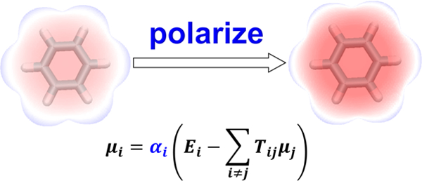
Graphical Abstract

1. Introduction

Polarizable force fields (FFs) play important roles in studying the structure, dynamics, and thermodynamics of many biomolecular systems due to their explicit treatment of electronic polarization effect.^1–4 They are also routinely applied in predicting the host-ligand binding affinities that are essential to the drug discovery process.^5–7 Interactive point dipole (IPD) models such as AMOEBA,⁸ AMBER,⁹ and SIBFA¹⁰ give each atom a point induced dipole, proportional to local electrical field strength and an atomic polarizability parameter α. Other means of estimating polarizability exist, e.g., fluctuating charges¹¹ and Drude oscillator models,^{4, 12} but those use their own parameters (albeit Drude models have been proven equivalent to IPD models after careful conversion¹²). The most widely used parameters are those of Thole¹³ and Swart,¹⁴ both of whom fit to modest sets of molecular polarizabilities (both experimental and computational) to obtain physically reasonable atomic polarizability values for the most common elements in organic chemistry.

While effective, these polarizability parameters leave room for improvement. Firstly, per-element atomic polarizabilities ignore the chemical environment that atoms are exposed to. For example, the current AMOEBA model uses element-based polarizability parameters supplemented with aromatic carbon and hydrogen types.¹⁵ Upon examining many organic molecular clusters, significant many-body polarization errors in this model were eliminated by the introduction of carbonyl-specific carbon and oxygen types.¹⁶ Secondly, polarizability parameters were often derived based on a small number of relatively small molecules. For example, in the original paper of Thole,¹³ about 20 molecules were employed. The polarizability parameters in the polarizable AMBER FF were derived initially based on 41 small molecules. In their later development, Wang and co-workers increased the number of molecules in training set to several hundreds.^17–18 Thirdly, the polarizability parameters have been mostly fitted to experimental or ab initio molecular polarizabilities. Reliance on a single source of data may cause over/underfitting of the model, especially when the data set is small.

Electrostatic potential (ESP) has been widely used by the FF developer community to obtain permanent charges¹⁹ and higher-order moments (such as dipole and quadrupole).⁸ Utilizing electrostatic potential responses to derive atomic polarizability parameters has also been demonstrated but without widespread adoption. For example, Kaminski et al. applied a series of electrostatic perturbations to the target molecules with dipoles (represented by two charges) at various locations around the molecule.^20–21 The atomic polarizability was then fitted to reproduce the ESP response upon perturbation. Elking et al. used a similar approach with a probe charge to derive atomic polarizabilities for their Gaussian induced dipole polarization model.²² Their results show that the ESP probing procedure outperforms the generic atom type-based molecular polarizability fitting. Although different in representation of polarizability effect, the polarizable Drude model by Mackerell and co-workers ²³ also uses a series of perturbed ESP maps to determine the polarizability parameters.

Here in this work, we combine both approaches, deriving Thole-style polarizability parameters by fitting against both molecular polarizabilities and ESP responses. For six elements (C, H, O, N, S, Cl) we are able to take advantage of 7211 molecular polarizabilities previously calculated at the LR-CCSD/d-aug-cc-pVDZ level.²⁴ This is supplemented with an additional set of over 300 molecules, including charged molecules and other heavy elements (F, Cl, Br, I, P), with molecular polarizabilities and ESP responses calculated at the MP2/aug-cc-pVTZ level.

By fitting to both sets of data (molecular polarizabilities and ESP responses), we: 1) avoid possible over/underfitting by solely targeting either set of data, and 2) examine the robustness of the model and transferability of the derived parameters by cross-validating on two sets of data. The current element-based atom types have been split to better reflect any given atom’s chemical environment, with the new types defined by SMARTS strings. Our results indicate that both individual sets of atomic polarizability parameters, as well as a hybrid model based on both data sets, can be used interchangeably to describe the molecular polarizability and ESP responses. The final set of parameters (based on the hybrid model) shows notable improvement over the current AMOEBA model, with the mean percentage molecular polarizability error being reduced from 9.3% to 2.5% and the RMS error from 1.24 ų to 0.40 ų for over 7200 molecules. Meanwhile, the RMS error of ESP responses has been reduced by 27%.

2. Method

2.1. Dipole interaction model

In the AMOEBA and AMOEBA+ models, an induced point dipole is introduced on the polarizable atom according to the electric field felt by that atom. Atomic polarization is obtained via an interactive induction model based on Thole’s damped interaction scheme.¹³

$${\mu }_i={\alpha }_i\left(E_i-\sum _{i\ne j}{T}_{ij}{\mu }_j\right)$$ Eq. 1

Where α_i is the atomic polarizability, E_i is the field felt by site i due to the multipole moments (charge, dipole and quadrupole) on other sites, and T_ij is the dipole field tensor (see e.g. Ref. ⁸). This interactive induction scheme requires that an induced dipole produced at any atom i will further induce other polarizable sites. The induced dipole on each polarizable atom is solved iteratively to obtain the converged induced dipole. It is worth mentioning that the dipole interaction matrix is damped to avoid the so-called polarization catastrophe²⁵ at very short interatomic distances. With a universal damping factor of 0.39 (with the exception of some metal cations²⁶), together with element-based isotropic atomic polarizability parameters, this model remains simple and shows reasonable transferability to describe the molecular polarizability of small organic molecules.¹⁵

2.2. Fitting targets: molecular polarizability and ESP responses

Molecular polarizability is a by-molecule description of how electron distribution changes in response to an external electric field. Experimental measurements exist for many molecules, as well as computational methods to estimate polarizability from quantum mechanical (QM) calculations.²⁷ The primary shortcoming is that there is no unique mapping of atomic polarizabilities to molecular polarizability, a problem aggravated when examining large molecules with many atoms contributing to overall polarizability.

Molecular electrostatic potential (ESP) has widely been used to optimize charges^28–29 and multipoles.^30–33 This is the energy a probe charge would feel at a given point in a fixed electrical field, such as that created by a molecule’s charge distribution. As such, it is often used as a proxy for electrostatic intermolecular interactions, with charges and multipoles fit to reproduce ESP on a grid surrounding the molecule.

Polarization can be thought of as the response of a molecule’s electron distribution (and thus its ESP) in response to an external electric field, such as that of another molecule. We add a small probe charge (+0.125 e) located at 4.3 Å away from the atom of interest, and permit the molecule’s electron distribution to relax to the presence of this probe charge, and re-calculate ESP. We note here that the combination of +0.125 e charge and 4.3 Å distance can provide large enough electronic response for later numerical fitting, and small enough to still result in linear polarization. The change in ESP from polarization is then the non-additivity in ESP between the probe-molecule system and its components (probe and unpolarized molecule) (Eq. 2). We then fit both to these $\mathrm{\Delta }{\phi }_{pol}$ values (ESP responses) and molecular polarizabilities up to quadrupole. An illustration of this approach is provided in Figure 1 using molecular surface of a benzene molecule colored by ESP values.

Figure 1.

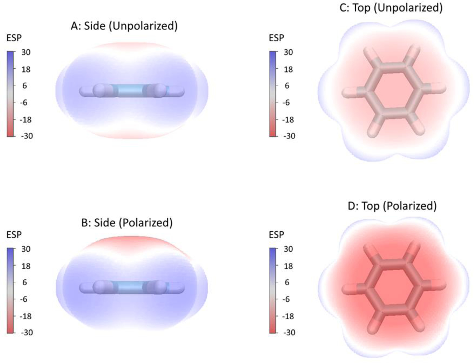
Molecular surface of benzene colored by electrostatic potential (ESP) in kcal/mol/e. (A,C) Unpolarized ESP surface and (B,D) Polarized ESP surface by the addition of a +1 electron charge above the ring (probe charge ESP not directly included). Calculations were performed at the MP2/aug-cc-pVTZ level using Gaussian 16 software.

$$\mathrm{\Delta }{\phi }_{pol}={\phi }_{Mol+pro}-{\phi }_{Mol}-{\phi }_{Pro}$$ Eq. 2

This approach has two advantages. First, the probe charge is a highly localized electrical disturbance: a dipole or other multipole would be even more strongly localized, but this is not explored in this work. Second, multiple probe locations can be used in independent calculations to probe near multiple locations of interest, e.g. near every non-redundant atom in the system.

2.3. Molecular databases

2.3.1. Molecular polarizability database

The molecular polarizability database includes a training set for parametrization and a validation set for validating the derived parameters. The training set contains 773 molecules in total, of which 700 molecules were chosen from the QM7b dataset according to chemical diversity, and the additional 73 molecules were constructed to expand the element coverage to F, Cl, Br, and I. The molecules in the QM7b set contain up to 7 heavy atoms (i.e., C, N, O, S, and Cl) with various levels of hybridization. The molecular polarizability for the 73 molecules was calculated at the MP2/aug-cc-pvtz level of theory. For the 700 molecules selected from QM7b set, the molecular polarizability data calculated at LR-CCSD/d-aug-cc-pVDZ level of theory was taken from Wilkins et al.²⁴ We show in the Results section that the differences between LR-CCSD/d-aug-cc-pVDZ and MP2/aug-cc-pvtz polarizabilities are within the uncertainty of our polarization model. The remaining 6511 molecules in the QM7b dataset were used as the validation set. Additionally, 422 molecules whose experimental molecular polarizabilities are available were added, of which less than 10% overlap with the QM7b set. Structures of these molecules were retrieved from PubChem API by molecular names provided in the publication of Bosque and Sales.³⁴ Structure optimization was performed using the Gaussian 09 or 16 software package³⁵ at MP2/6–31G* ³⁶ level of theory; MP2/6–311G* was used for iodine-containing molecules.

2.3.2. ESP probing database

We constructed a set of molecules for ESP probing. Due to the computational cost, a minimal set of molecules that cover all the atom types of the molecular polarizability set was selected. In total, 316 probing structures were generated for 37 small molecules, with each molecule being probed at several different locations outside of the van der Waals sphere by an external charge (+0.125 e). The ESP of these probe structures was evaluated at MP2/aug-cc-pvtz³⁷ level; The def2-tzvppd ^38–39 basis set was used for iodine-containing molecules. This basis set was obtained from the basis set exchange library.⁴⁰

2.3.3. Charged molecule database

Like the neutral molecules described above, we also constructed molecular polarizability and ESP probing datasets for charged molecules commonly encountered in (bio)chemistry. In total, we performed QM polarizability calculations for 70 molecules with either positive or negative charges, of which 27 molecules were used to generate the ESP probing data. Polarizability and ESP were calculated at the same level as the neutral molecules.

3. Results and discussion

3.1. Atom types for atomic polarizability

String-based specifications are widely used in cheminformatics and computational chemistry as molecular descriptors. Here we adopt SMARTS patterns⁴¹ to define atom types for the atoms in neutral molecules. Every atom matching a given atom type shares one atomic polarizability parameter. In total, we found that 34 atom types can cover the chemistry of over 7600 molecules (both QM and experimental datasets) used in this work. Whereas current AMOEBA polarizability types are generally limited to one aliphatic and one aromatic type (see Supporting Information, SI, Table S1), the current set includes multiple aliphatic types for many elements. The exact SMARTS patterns are listed in Table S2. For charged molecules, the atom types were defined based on the connectivity of the atoms. A detailed illustration of the atom types for the charged molecules is shown in Figure S1.

3.2. Comparison of CCSD and MP2 polarizability

To check whether the literature LR-CCSD/d-aug-cc-pVDZ level²⁴ was consistent with our own MP2/aug-cc-pVTZ level, we randomly selected 52 molecules from the QM7b database for comparison. Molecular polarizabilities were re-calculated at MP2/aug-cc-pVTZ level, using the QM7b geometry. The result shows that difference between these two levels of QM theory is only 0.05 ų on average for the isotropic molecular polarizability (Table S3), which is within the uncertainty of a classical polarizability model. This suggests that we can safely use two levels of QM molecular polarizabilities as the fitting target.

3.3. Atomic polarizability derived from fitting molecular polarizability

As described above, the atomic polarizability was first derived by fitting the QM molecular polarizability on the training set data. The resulted atomic polarizability parameters (denoted as fit-polar set) are listed in Table 1. This fit-polar set represents several changes compared to the current parameters of the AMOEBA model (Table S1). For example, the aromatic carbon is increased from 1.75 to 2.11 ų; the sp hybridized carbon is now 2.28 ų; similarly, nitrogen on aromatic systems also increases from 1.07 to 1.65 ų). However, many other polarizability parameters show only small changes versus the current AMOEBA model.

Table 1.

Atomic polarizabilities (in ų) obtained from fitting against molecular polarizabilities (fit-polar) and electrostatic potential responses (fit-esp) respectively. The final parameters are the result of averaging fit-polar and fit-esp sets.

Index	Atom type	Short description a	fit-polar	fit-esp	final
1	HW	Water H	0.43000	0.43190	0.42830 b
2	Har	H on aromatic and double bonded atoms	0.45938	0.40413	0.43175
3	Hnonpol	H on carbon atoms	0.47085	0.48982	0.48034
4	Hpolar	H on N, O, S, and halogens	0.47167	0.44294	0.45730
5	Car	Aromatic and double bonded C	2.11333	2.01569	2.06451
6	Cch4	Methane C	1.33467	1.34778	1.34123
7	Cnonpol	Nonpolar C	1.45458	1.37539	1.41499
8	Cpolar	Polar C	1.65038	1.58890	1.61964
9	Csp	Triple bonded C	2.27642	2.12827	2.20235
10	Nnh3	Ammonia N	1.07512	1.23636	1.15574
11	Nar	Aromatic N	1.64607	1.75761	1.70184
12	Nnonpol	N on C atoms	1.23564	1.13368	1.18466
13	Npolar	N on non-carbon atoms	1.44144	1.44604	1.44374
14	Nsp	Triple bonded N	1.15924	1.15674	1.15799
15	Nsp2	Double bonded N	1.19623	1.29033	1.24328
16	OW	Water O	0.97102	0.97393	0.97635 b
17	Oar	Aromatic O	0.83226	0.83226	0.83226
18	Ononpol	O on carbon atoms	0.81831	0.80617	0.81224
19	Opolar	O on other atoms	0.85184	0.86322	0.85753
20	Ohacid	O of acid (with H)	0.81831	0.84635	0.83233
21	Osp2c	O on carbonyl	0.85551	0.97202	0.91377
22	O-sulf	O single bonded S	0.83413	0.85888	0.84651
23	O=sulf	O double bonded S	0.83394	0.88365	0.85880
24	Sar	Aromatic S	3.27951	3.13221	3.20586
25	Snonpol	S on carbon atoms	3.54925	3.26305	3.40615
26	Spolar	S on other atoms	2.99663	2.99151	2.99407
27	Fnonar	Nonaromatic F	0.36896	0.32725	0.34810
28	Far	Aromatic F	0.29050	0.32680	0.30865
29	Clar	Aromatic Cl	2.58795	2.54576	2.56686
30	Clnonar	Nonaromatic Cl	2.36596	2.30821	2.33709
31	Brar	Aromatic Br	4.20104	4.06331	4.13218
32	Brnonar	Nonaromatic Br	3.57711	3.47471	3.52591
33	Iar	Aromatic I	5.48163	5.48163	5.48163
34	Inonar	Nonaromatic I	5.42354	5.42354	5.42354

^a.Refer to Table S2 for the full description and SMART patterns

^b.Final atomic polarizability parameters of water (atom type: HW and OW) were made consistent with the optimized values using both gas and liquid water properties.⁵¹

The performance of this set of parameters (fit-polar) is summarized in Table 2. The statistics are calculated on the three polarizability eigenvalues (denoted as α_ii in Table 2) and the isotropic molecular polarizabilities (denoted as α_iso in Table 2). For the training set, the Root Mean Square Error (RMSE) and Unsigned Mean Percentage Error (UMPE, defined in Eq. 3) are 0.85 ų and 4.7%, respectively, on the three eigenvalues α_ii, and 0.41 ų and 2.8%, respectively, on the isotropic polarizability α_iso. This performance quality is well maintained (Table 2) on the much larger validation set, which demonstrates a robust, transferable model unlikely to be suffering from overfitting problems.

Table 2.

Performance of the fit-polar set of parameters on the training and validation polarizability sets. Root mean square error (RMSE, in ų) and unsigned mean percentage error (UMPE, defined in Eq. 3) are reported.

Statistics a,b	Training set (773 molecules)	Validation set (6511 molecules)
RMSE (αii)	0.85	0.78
UMPE (αii)	4.7%	4.4%
RMSE (αiso)	0.41	0.39
UMPE (αiso)	2.8%	2.6%

^a.α_ii: statistics based on three eigenvalues, where $i=x,y,z$.

^b.α_iso: statistics based on the isotropic polarizabilities, i.e., $\frac{1}{3}\left({\alpha }_{xx}+{\alpha }_{yy}+{\alpha }_{zz}\right)$.

$$\text{UMPE}\left(\alpha \right)=\frac{1}{N}\sum _N\frac{\left|\alpha -{\alpha }_{ref}\right|}{{\alpha }_{ref}}*100\%$$ Eq. 3

Where N loops over the number of molecules and α is the molecular polarizability (either α_ii or α_iso).

3.4. Atomic polarizability derived from fitting electrostatic potential

Atomic polarizability parameters were also derived from fitting the ESP responses as described in the Methods section. As seen in Table 1 (fit-esp set), generally, these parameters are slightly smaller than their fit-polar counterparts. Exceptionally, for several nitrogen and oxygen types, the fit-esp set of atomic polarizability parameters become bigger than the fit-polar set. This can easily be attributed to the lone pair of nitrogen and oxygen atoms in these molecules. Fitting to electrostatic potential tends to increase the polarizability to capture the polarization due to external field along the direction of the lone pair.

The performance of this set of parameters has been summarized in Table 3. The RMS error of ESP responses is 0.0326 kcal/mol/e. We directly apply this set of parameters to the polarizability dataset and find the resulting parameters are approximately as effective as the fit-polar set (Table 3).

Table 3.

Performance of the fit-polar, fit-esp, final and the current AMOEBA sets of polarizability parameters on the ESP and molecular polarizability sets. Root mean square error (RMSE, in kcal/mol/e for ESP and in ų for polarizability) and unsigned mean percentage error (UMPE, defined in Eq. 3) are reported.

Parameters	ESP set (316 probing structures)		Polarizability set a,b (7284 molecules)
fit-polar	RMSE	0.0347	RMSE (αii)	0.79
			UMPE (αii)	4.5%
			RMSE (αiso)	0.39
			UMPE (αiso)	2.6%
fit-esp	RMSE	0.0326	RMSE (αii)	0.81
			UMPE (αii)	4.2%
			RMSE (αiso)	0.43
			UMPE (αiso)	2.6%
final	RMSE	0.0333	RMSE (αii)	0.79
			UMPE (αii)	4.2%
			RMSE (αiso)	0.40
			UMPE (αiso)	2.5%
AMOEBA	RMSE	0.0451	RMSE (αii)	1.54
			UMPE (αii)	8.8%
			RMSE (αiso)	1.24
			UMPE (αiso)	9.3%

^a.α_ii: statistics based on three eigenvalues, where $i=x,y,z$.

^b.α_iso: statistics based on the isotropic polarizabilities, i.e., $\frac{1}{3}\left({\alpha }_{xx}+{\alpha }_{yy}+{\alpha }_{zz}\right)$.

3.5. Finalization of atomic polarizability

As described above, two sets of atomic polarizability parameters have been derived by fitting to either molecular polarizability or the change of ESP due to an external field. Results show that the two sets of parameters have very similar quality metrics (Table 3), which is partly due to very similar parameters for most polarizability types. For the atoms with lone pair electrons such as oxygen and nitrogen, the atomic polarizability must be bigger to capture the polarization of ESP in the direction of lone pairs. These results suggest that the ESP information should not be excluded in the derivation of atomic polarizability, as ESP captures these outliers where molecular polarizability does not. Our final polarizability parameters are a simple average of the two sets of parameters (denorted as final set in Table 1).

The testing results on the whole molecular polarizability and ESP databases are listed in Table 3. As expected, the averaged parameters maintain performance very similar to the component fit-polar and fit-esp sets. In addition, all sets of parameters outperform the current AMOEBA model. The current AMOEBA gives an RMS error of 1.24 ų for the mean polarizability of 7284 molecules in the polarizability set, which is reduced to 0.40 ų in this study with updated atomic polarizabilities. Nearly 4-fold improvement can be seen from the unsigned mean percentage error (9.3% vs. 2.5%, Table 3, Figures 2 and 3). The correlation coefficient (R²) for the mean molecular polarizability by this work improves from 0.74 to 0.92. As seen from Table 3 and Figure 3, a higher RMS error is obtained when checking the three eigenvalues of the molecular polarizability. Specifically, large errors present for large molecules such as those with highly conjugated rings and long chains. For these systems, neither the current nor the updated set of parameters result as good performance as for the small molecules. This is well expected and acceptable given that AMOEBA adopts the simple isotropic atomic polarizability model¹³ and a limited number of atom types are employed in this work. Further improvements may require the use of anisotropic atomic polarizabilities⁴² and finer atom type definitions.

Figure 2.

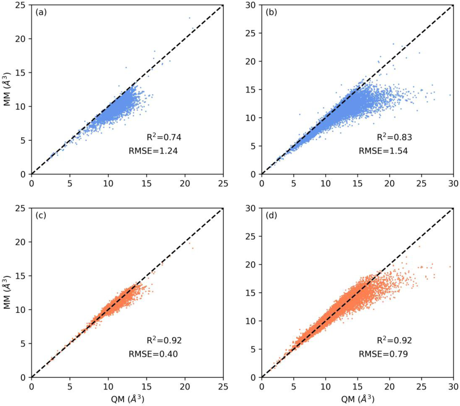
Correlation between QM and MM molecular polarizabilities. The MM model values were calculated with two sets of parameters (blue: current AMOEBA; orange: this work). Both the isotropic molecular polarizability (a) and (c), and three eigenvalues (b) and (d) are plotted. Black dotted lines represent perfect correlation. Correlation coefficient (R²) and RMSE values (in ų) are reported.

Figure 3.

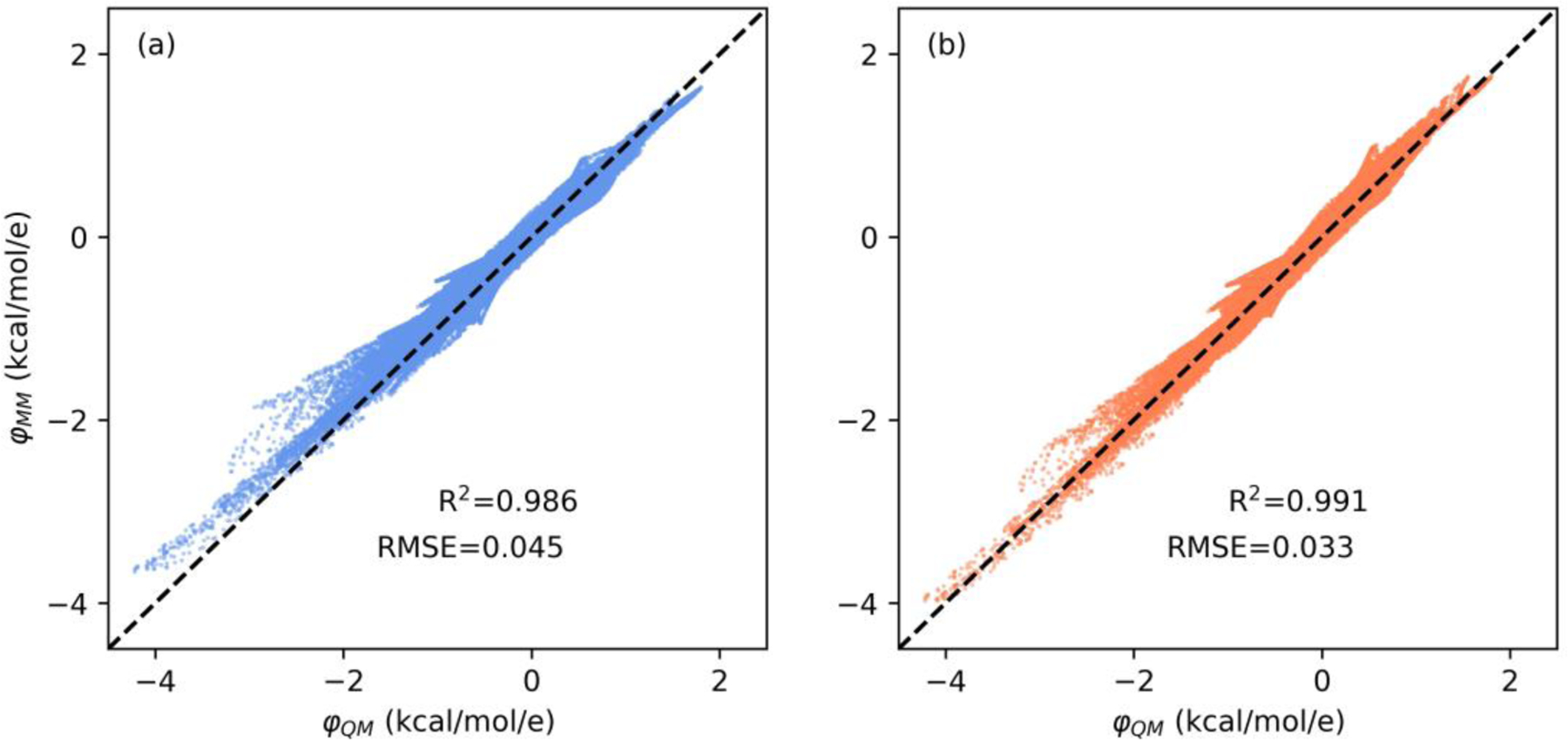
Correlation between the QM and MM electrostatic potential changes due to external field (i.e. ESP responses). The MM values were calculated with two sets of parameters: (a) the current AMOEBA, and (b) this work. Black dotted lines represent perfect correlation. Correlation coefficient (R²) and RMS error (in kcal/mol/e) values are reported.

In addition, the final set of parameters have been tested on several gas molecules as special cases (Table S4) and 422 organic molecules with experimental molecular polarizability data (Table S5). The result shows that one can directly apply these parameters without defining new atom types for the gas molecules. For the organic molecules, the RMSE and UMPE are 0.49 ų and 2.9%, respectively. The level of accuracy is similar to the QM set with over 7200 molecules, indicating the transferability of the derived atomic polarizability parameters.

It is believed that the atomic polarizability reflects the spheric “volume” of an atom, not unsurprising given that polarizability parameters are defined in units of volume.⁴³ Correlating the polarizability parameters with atomic and covalent radii suggests polarizability is better correlated with atomic radii (Figure 4). Particularly, polarizability for fluorine is 0.33 ų on average, smaller than that of hydrogen (0.45 ų). This trend is in line with the atomic radii of two atoms (0.42 Å for fluorine vs. 0.53 Å for hydrogen). Polarizability for the heavy aromatic atom types is usually higher than non-aromatic ones (e.g., C, N, Cl, Br, and I), which is in line with our chemical intuition that the electrons are more delocalized in the aromatic than non-aromatic systems. Atoms with type “Xpolar” have higher polarizability than those with “Xnonpol” (where X = C, N and O), which is consistent with chemistry that one atom connecting to electronegative atoms (N and O) is more polarizable than the one that connects to a carbon. These results suggest that the polarizability parameters we derived here are physically meaningful, as higher polarizability correlates with larger, more delocalized electron densities.

Figure 4.

Correlation between the final atomic polarizability parameters and atomic radius (orange circles) or covalent radius (blue triangles). Polarizability parameters are averaged over atom types for each element. Solid lines are the linear fit of the data. Atomic and covalent radii are taken from Ref. 49 and 50, respectively.

3.6. Effect of polarizability on the many-body energy

Non-additive many-body interactions are responsible for various condensed phase properties. It has been of interest to examine the agreement of many-body interaction energy by polarizable models and high-level quantum chemical calculations.^{16, 44–45} Here we calculate the 3-body energy by AMOEBA model with the current and the final set of polarizability parameters and compare them with the high-quality benchmark data obtained at CCSD(T)/CBS level of theory for the 3B-69 dataset.⁴⁶ Our results show that the AMOEBA model with the current element-based polarizability parameters captures the 3-body energy quite well with an RMS error of 0.30 kcal/mol (Table S6). The agreement can be slightly improved with an RMS error of 0.26 kcal/mol when the final set of polarizability parameters are used. These parameters will be further examined in MD simulations of condensed phase in the future.

3.7. Atomic polarizability for charged molecules

Following the same procedure of deriving parameters for neutral molecules, atomic polarizability parameters for common charged molecules have been generated. Due to the formal charge, it is sometimes difficult to use SMARTS strings to define the atom types of these molecules. In this work, we developed a program to enumerate the possible charged fragments to assign the atom types. The parameters and performance for charged molecules are provided in Table S7 and S8, respectively. For the charged molecules, an RMSE of 0.52 ų and UMPE of 3.1% for the isotropic polarizability are obtained with the final set of parameters. The slight reduction in fit quality (compared with the neutral set) may partially be explained by the difficulty in fitting the significantly larger absolute polarizability values in charged groups, particularly negatively charged groups with diffuse electron clouds.

4. Conclusion

We have derived three sets of atomic polarizability parameters for use with interactive point dipole models. One set is from direct fitting to the molecular polarizability calculated from high-level quantum chemistry calculations. The second set is from fitting the electrostatic potential change due to an external electric field introduced by a dummy partial charge. The final set is obtained by averaging these values, which fortunately are in close correspondence. Our results clearly show that two sets of approaches to deriving atomic polarizability parameters are closely matched, though the ESP approach is more effective in capturing polarization in the direction of the lone pairs of atoms such as nitrogen and oxygen atoms. With the newly derived atomic polarizability parameters, we show that for the QM set with over 7200 molecules, the RMS isotropic molecular polarizability error is reduced from 1.24 ų (current AMOEBA model) to 0.40 ų. This level of accuracy is achieved through introducing additional polarizability types to Thole’s interactive induction scheme to consider both element and local electronic environment of the atoms. It is worth mentioning that the universal damping factor (0.39) determined by AMOEBA model ⁸ remains the same in this work. Testing of the final parameters on the available experimental polarizability set (422 molecules) results in an RMS error of 0.49 ų, indicating the good transferability of the derived set of atomic polarizability parameters. Using the same procedure, we have also derived the atomic polarizability parameters for 70 molecular ions, which expands the applicability of the polarizability model.

A Python program was developed to assign polarizability parameters from a SMARTS string, available on Github.⁴⁷ The final set of atomic polarizability parameters has also been incorporated into the PolType2 automation tool ⁴⁸ for AMOEBA-family FF development. The parameters derived in this work will be used in future AMOEBA⁸ and AMOEBA+ ³³ force fields, and can easily be used in other Thole-type polarization models, and with slightly more effort, in Drude oscillator models.¹²