A penalization approach to random-effects meta-analysis

Summary

Systematic reviews and meta-analyses are principal tools to synthesize evidence from multiple independent sources in many research fields. The assessment of heterogeneity among collected studies is a critical step when performing a meta-analysis, given its influence on model selection and conclusions about treatment effects. A common-effect (CE) model is conventionally used when the studies are deemed homogeneous, while a random-effects (RE) model is used for heterogeneous studies. However, both models have limitations. For example, the CE model produces excessively conservative confidence intervals with low coverage probabilities when the collected studies have heterogeneous treatment effects. The RE model, on the other hand, assigns higher weights to small studies compared to the CE model. In the presence of small-study effects or publication bias, the over-weighted small studies from a RE model can lead to substantially biased overall treatment effect estimates. In addition, outlying studies may exaggerate between-study heterogeneity. This article introduces penalization methods as a compromise between the CE and RE models. The proposed methods are motivated by the penalized likelihood approach, which is widely used in the current literature to control model complexity and reduce variances of parameter estimates. We compare the existing and proposed methods with simulated data and several case studies to illustrate the benefits of the penalization methods.

1 |. INTRODUCTION

Meta-analysis is a set of statistical methods for synthesizing evidence from a collection of multiple independent studies on a common scientific question. The application of meta-analysis has become a powerful tool in many scientific areas.^1,2,3,4 Though not always the case, conventionally, meta-analyses are implemented via either the common-effect (CE) or random-effects (RE) model.^5,6,7 The CE model assumes that each study shares a common true effect size; i.e., all studies are homogeneous. However, in practice, studies frequently differ in terms of study and patient characteristics, such as patient selection and baseline disease severity, among others.^8,9 In such situations, the RE model is used to account for systematic heterogeneity between studies.

To select an appropriate meta-analytic model, it is critical to accurately measure the heterogeneity among the collected studies. Many methods have been proposed to detect and measure such heterogeneity. A classic assessment of heterogeneity is the Q test.^10,11 It has low statistical power when the number of studies in a meta-analysis is small, and we cannot depend entirely on the Q test for selecting the CE or RE model.^12,2 In addition, the Q statistic is influenced by the number of studies, while the between-study variance depends on the scale of measurement. Several alternative methods, such as the I² and R_I statistics, have been proposed to quantify heterogeneity.^{12,13,14,15,16} Despite their widespread use in applied meta-analyses, these methods are subject to several important limitations. For example, the I² and R_I statistics should not be used as an absolute measure.^17,18,19,20 As the studies’ sample sizes increase, these measures would approach 100%. This issue may be addressed by the between-study coefficient of variation, CV_B, proposed by Takkouche et al.^12,18; it is the ratio of the between-study standard deviation (SD) estimate divided by the random-effect meta-estimate. Recent literature advocates reporting prediction intervals for a future study alongside conventional confidence intervals (CIs) of overall treatment effects to properly describe heterogeneity. Such intervals incorporate the between-study variance and represent the range of future study results.^21,22,23,24

The aforementioned approaches are based on either the CE or RE model. The CE model produces CIs with poor coverage probabilities when studies have heterogeneous effect sizes.²⁵ On the other hand, the estimate of the overall effect size produced by the RE model may be more biased compared to that of the CE model in the presence of publication bias or small-study effects.²⁶ Alternative methods, which are neither the conventional CE nor RE model, have been proposed.^26,27,28,29 These methods use the CE model to yield a point estimate, obtaining robustness to publication bias, and use the RE model to compute its CI for maintaining a nominal coverage probability.

We propose a novel penalized method to naturally balance between the CE model and RE model. The benefit of penalized likelihood has been extensively studied and applied in high-dimensional data analysis to control model complexity and reduce variances of parameter estimates.^30,31 In the context of linear regression, when the penalty on regression coefficients increases, estimates of small coefficients shrink toward 0, removing nuisance variables and achieving variable selection. This article considers penalty terms for the between-study variance in a meta-analysis to select an optimal estimate. When no penalty is applied to the between-study variance, the proposed method is identical to the RE model. When the penalty is large enough, the estimated between-study variance shrinks toward 0, and the proposed method reduces to the CE model. Therefore, the new method pursues a trade-off between the conventional CE and RE models. It is useful in the presence of outlying studies that may lead to an overestimation of between-study variance.

This article is organized as follows. Section 2 presents four meta-analyses with and without potential outlying studies. Section 3 presents a brief review of conventional methods to assess heterogeneity, introduces and illustrates the penalization methods, and provides loss functions for selecting an optimal estimate. In Section 4, we evaluate the performance of the proposed and existing methods, and Section 5 applies these methods to the four examples of meta-analyses presented in Section 2. Section 6 closes with a brief discussion.

2 |. EXAMPLES

This section presents four real meta-analyses, all of which are publicly available in the Cochrane Library. The first meta-analysis, consisting of 21 studies, was reported by Bohren et al.³² to investigate the effects of continuous, one-to-one intrapartum support on spontaneous vaginal births, compared with usual care. The second meta-analysis was reported by Storebø et al.³³ to assess the effect of methylphenidate on serious adverse events for children and adolescents with attention deficit hyperactivity disorder; it included a total of 20 studies. The third meta-analysis, also consisting of 20 studies, was reported by Carless et al.³⁴ to assess the efficacy of platelet-rich-plasmapheresis in reducing peri-operative allogeneic red blood cell transfusion in cardiac surgery. The fourth meta-analysis, consisting of 53 studies, was conducted by Bjelakovic et al.³⁵ to assess beneficial and harmful effects of vitamin D supplementation for the prevention of mortality in healthy adults and adults in a stable phase of disease. The second meta-analysis measured treatment effects using risk ratios (RRs); the remaining three meta-analyses all used odds ratios (ORs). Both RRs and ORs were analyzed on a logarithmic scale.

Figure 1 presents forest plots of these four meta-analyses, which present their study-specific observed effect sizes and their 95% CIs. They suggest high between-study variability among studies, both in magnitude and direction. For example, in the first meta-analysis, study 18 has a wide 95% CI, which does not overlap with the CIs of the overall OR produced by both the CE and RE models. Similarly, in the second meta-analysis, the 95% CI of study 16 does not overlap with the CIs of the overall RR produced by both the CE and RE models. The fourth meta-analysis perhaps contains the most heterogeneous studies among the four case studies; more than 10 studies’ CIs do not overlap with the CIs of the overall OR produced by both the CE and RE models.

FIGURE 1.

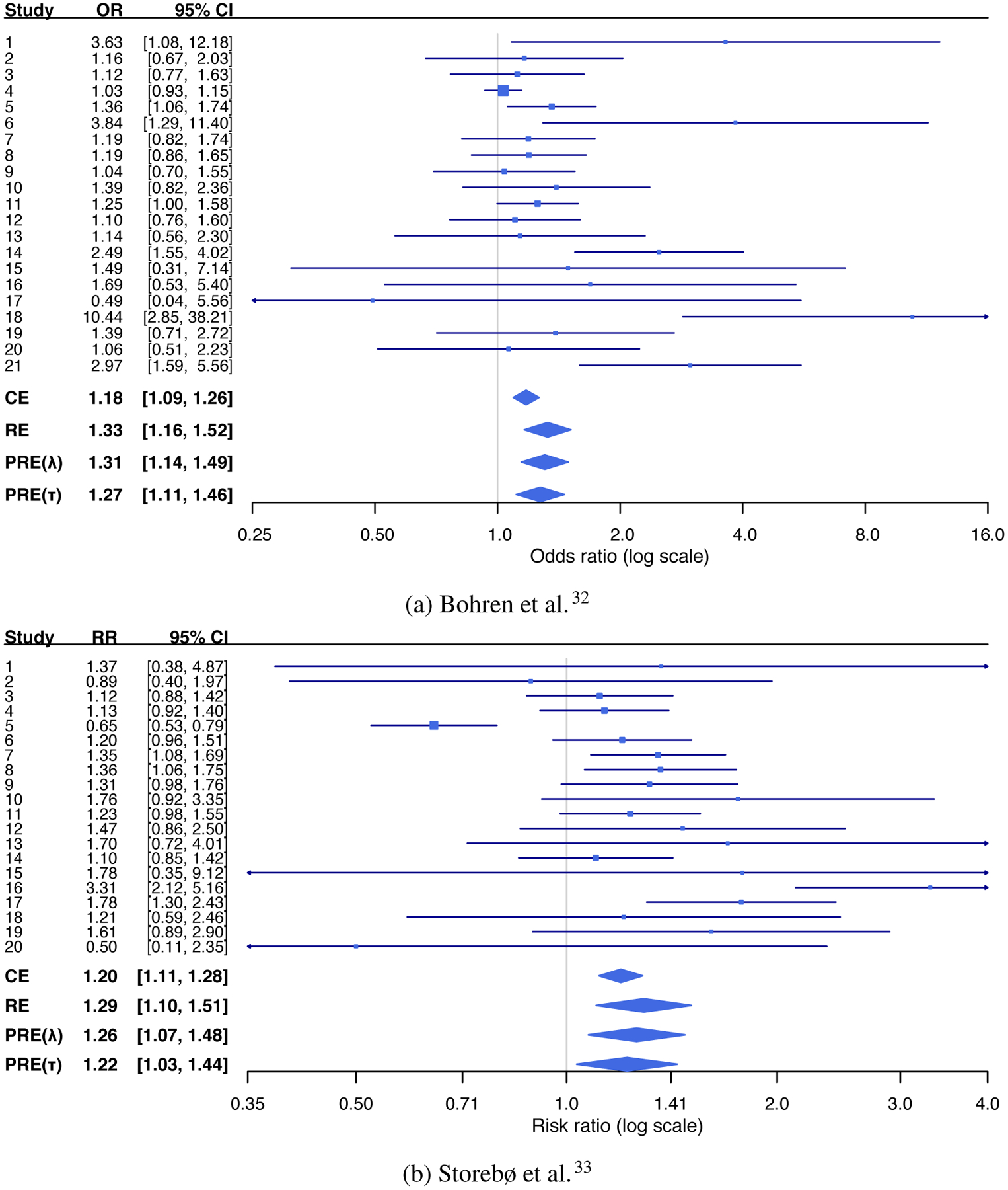
Forest plots of the four examples of meta-analyses.

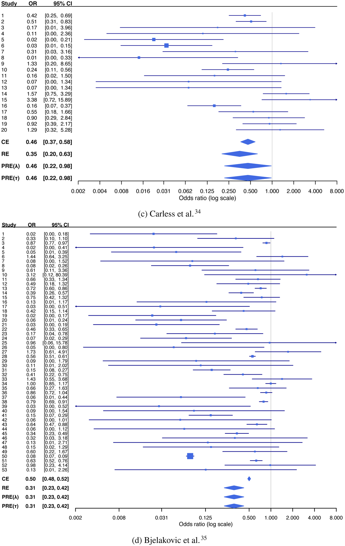
To detect potential outliers, we apply diagnostic procedures to the four meta-analyses under both CE and RE settings.^36,37 These procedures are based on the study-specific standardized residuals, which are expected to be approximately normally distributed when no outliers are present. Studies with standardized residuals larger than 3 in absolute magnitude may be considered outliers. Figure 2 shows plots of standardized residuals of the four meta-analyses. In Figure 2(a), the standardized residual of study 4 is less than −3 under both CE and RE settings; study 18’s standardized residual is greater than 3 under both settings. These two studies might cause the between-study variance to be overestimated. The p-value of the Q test is 0.119 after excluding studies 4 and 18, whereas the p-value is 0.001 in the original dataset. In Figure 2(b), the standardized residual of study 5 is less than −3 under both CE and RE settings; study 16’s standardized residual is greater than 3 under both settings. The p-value of the Q test is 0.697 after excluding studies 5 and 16, whereas the p-value is far less than 0.001 in the original dataset. Figure 2(c) indicates two outliers identified under the CE setting but no outliers under the RE setting in the third meta-analysis. Figure 2(d) indicates eight outliers identified under the CE setting but no outliers under the RE setting.

FIGURE 2.

Plots of study-specific standardized residuals of the four examples of meta-analyses under the common-effect (denoted by filled triangles) and random-effects (denoted by unfilled dots) settings. The plus signs represent truncated standardized residuals whose absolute values are greater than 5.

3 |. METHODS

3.1 |. Existing methods

Suppose a meta-analysis collects n independent studies. Let μ_i be the true effect size in study i (i = 1, …, n). Each study reports an estimate of the effect size and its sample variance, denoted by y_i and $s_i^2$, respectively. These data are commonly modeled as $y_i~N\left({\mu }_i,s_i^2\right)$. Although $s_i^2$ is subject to sampling error, it is usually treated as a fixed, known value. This assumption is generally valid if each study’s sample size is large. If study-specific true effect sizes are assumed ${\mu }_i\stackrel{\text{ iid }}{~}N\left(\mu ,{\tau }^2\right)$, this is the RE model, where μ is the overall effect size and τ² is the between-study variance. If τ² = 0 and thus μ_i = μ for all studies, this implies that studies are homogeneous and the RE model is reduced to the CE model.

The Q statistic is widely used to test for the homogeneity among the studies (i.e., H₀ : τ² = 0). Specifically, $Q={\sum }_{i=1}^n{w}_i{\left(y_i-\overline{y}\right)}^2$, and it approximately follows a ${\chi }_{n-1}^2$ distribution under the null hypothesis. Here, $w_i=1/s_i^2$ and $\overline{y}={\sum }_{i=1}^n{w}_i{y}_i/{\sum }_{i=1}^n{w}_i$. If the studies are assumed to be heterogeneous, it is critical to estimate the between-study variance τ². Various estimators of τ² are available. A popular choice is the method-of-moments (MOM) estimator.¹⁰ The MOM estimator performs well when τ² is small, but it can underestimate the true heterogeneity when τ² is large and the number of studies is small, leading to substantial bias.^38,39,40 Several alternative estimators, such as those based on the maximum likelihood (ML) and the restricted maximum likelihood (REML), may be suitable alternative choices.^41,42

3.2 |. Penalizing the between-study variance

We propose a new approach to estimating the overall effect size in a meta-analysis by penalizing the between-study variance when the heterogeneity is overestimated. Marginally, the RE model yields $y_i~N\left(\mu ,s_i^2+{\tau }^2\right)$, and its log-likelihood is

$$\ell \left(\mu ,{\tau }^2\right)=-\frac{1}{2}\sum _{i=1}^n\left[\text{log}\left(s_i^2+{\tau }^2\right)+\frac{{\left(y_i-\mu \right)}^2}{s_i^2+{\tau }^2}\right]+C,$$

where C is a constant. The ML estimates of μ and τ² can be obtained by maximizing ℓ(μ, τ²), or equivalently,

$$\left({\widehat{\mu }}_{\text{ML}},{\widehat{\tau }}_{\text{ML}}^2\right)=\underset{\mu ,{\tau }^2\ge 0}{\text{arg}\text{min}}\sum _{i=1}^n\left[\text{log}\left(s_i^2+{\tau }^2\right)+\frac{{\left(y_i-\mu \right)}^2}{s_i^2+{\tau }^2}\right].$$ (1)

In the past two decades, penalization methods have been rapidly developed for variable selection in high-dimensional data analysis to control model complexity and reduce variances of parameter estimates. Such methods aim at removing nuisance variables by applying various penalty functions to shrink their regression coefficients toward 0. In the context of mixed-effects models, Bondell et al.⁴³ use penalization methods in linear models for simultaneous selecting fixed and random effects; Ibrahim et al.⁴⁴ extend them to generalized linear models.

Borrowing the idea from the penalization methods, we employ a penalty term on the between-study variance τ² in the setting of meta-analysis. The penalty term increases with τ². Specifically, we consider the following optimization problem:

$$\left(\widehat{\mu }(\lambda ),{\widehat{\tau }}^2(\lambda )\right)=\underset{\mu ,{\tau }^2\ge 0}{\text{arg}\text{min}}\left\{\sum _{i=1}^n\left[\text{log}\left(s_i^2+{\tau }^2\right)+\frac{{\left(y_i-\mu \right)}^2}{s_i^2+{\tau }^2}\right]+\lambda p\left({\tau }^2\right)\right\},$$ (2)

where p(τ²) is a penalty function for τ² and λ ≥ 0 is a tuning parameter that controls the penalty strength. Generally, the penalty function should have the minimum value at τ² = 0, thus the estimate ${\widehat{\tau }}^2(\lambda )$ shrinks toward 0 when λ is large. Different penalty functions may be used, which in turn may result in different estimates. Regardless of the choice of the penalty function, the estimated between-study variance is expected to have a decreasing trend as λ increases. Unlike the penalty function used for variable selection, we aim to apply the penalty function in a meta-analysis to reduce the overestimation of heterogeneity. In this sense, the choice of the penalty function for a meta-analysis might play a less critical role as in the context of variable selection; see more details in Section 3.4. This article primarily considers p(τ²) = τ² to illustrate the penalization methods.

Using the technique of profile likelihood by taking the target function’s derivative in Equation (2) with respect to μ for a given τ²,⁴⁵ the optimization is achieved at

$$\tilde{\mu }\left({\tau }^2\right)=\frac{{\sum }_{i=1}^n{y}_i/\left(s_i^2+{\tau }^2\right)}{{\sum }_{i=1}^{n}1/\left(s_i^2+{\tau }^2\right)}.$$

The bivariate optimization problem is reduced to a univariate minimization problem:

$$\begin{gathered} {\widehat{\tau }}^2(\lambda )=\underset{{\tau }^2\ge 0}{\text{arg}\text{min}}\left\{\sum _{i=1}^n\left[\text{log}\left(s_i^2+{\tau }^2\right)+\frac{{\left(y_i-\tilde{\mu }\left({\tau }^2\right)\right)}^2}{s_i^2+{\tau }^2}\right]+\lambda p\left({\tau }^2\right)\right\}; \\ \widehat{\mu }(\lambda )=\tilde{\mu }\left({\widehat{\tau }}^2(\lambda )\right)=\frac{{\sum }_{i=1}^n{y}_i/\left(s_i^2+{\widehat{\tau }}^2(\lambda )\right)}{{\sum }_{i=1}^{n}1/\left(s_i^2+{\widehat{\tau }}^2(\lambda )\right)}. \end{gathered}$$ (3)

When λ = 0, the minimization problem in Equation (2) is equivalent to that in Equation (1), so the penalized-likelihood method is identical to the conventional RE model. By contrast, it can be shown that a sufficiently large λ produces the estimated between-study variance as 0, leading to the conventional CE model; see Appendix A.1. Therefore, a moderate tuning parameter λ corresponds to a trade-off between the CE and RE models.

3.3 |. Selection of the tuning parameter λ

As different tuning parameters lead to different estimates of $\widehat{\mu }(\lambda )$ and ${\widehat{\tau }}^2(\lambda )$, it is important to select the optimal λ among a set of candidate values. We perform the cross-validation process and construct a loss function of λ to measure the performance of specific λ values. The λ corresponding to the smallest loss is considered optimal.

Because λ ∈ [0, +∞) does not have an upper bound in theory, meta-analysts may only consider a finite number of candidate values, calculate their respective loss functions, and select the corresponding optimal λ. If the range of candidate values is too narrow, the true optimal λ may be beyond the constructed range and thus is missed by the cross-validation. On the other hand, if the range is too wide, all candidate values may have large gaps, producing the possibility that the optimal λ is within a certain gap and away from the selected candidate values. Therefore, to implement the cross-validation in practice, a reasonable range of potential λ values is required. Appendix A.1 provides a threshold, denoted by λ_max, based on the penalty function p(τ²) = τ². For all λ > λ_max, the estimated between-study variance is 0. Consequently, we may select a certain number of candidate values (say, 100) from the range [0, λ_max] for the tuning parameter.

For a set of candidate tuning parameters, the leave-one-study-out (i.e., n-fold) cross-validation is used to obtain the loss function, defined as

$$L(\lambda )={\left[\frac{1}{n}\sum _{i=1}^n\frac{{\left(y_i-{\widehat{\mu }}_{(-i)}(\lambda )\right)}^2}{s_i^2+{\tau }^2+\text{Var}\left({\widehat{\mu }}_{(-i)}(\lambda )\right)}\right]}^{1/2}.$$ (4)

The subscript (−i) indicates that study i is removed. The loss function is essentially the square root of the average of study-specific squared standardized residuals. In each element of the summation, the numerator represents study i’s residual. The overall effect size is estimated using all studies except study i; if study i is a potential outlier, this procedure removes its potential impact on the overall effect size estimate. The denominator in Equation (4) is the sum of two variance components: the marginal variance of y_i and the variance of ${\widehat{\mu }}_{(-i)}(\lambda )$. The two variance components are based on study i and the remaining n − 1 studies accordingly; they are statistically independent. Because each study’s standardized residual approximately follows the standard normal distribution under the true model, the loss function is expected to be close to 1.

More specifically, for a given λ and using all data except that from study i, the estimated between-study variance, ${\widehat{\tau }}_{(-i)}^2(\lambda )$, can be obtained from Equation (3), so the overall effect size is estimated as:

$${\widehat{\mu }}_{(-i)}(\lambda )=\frac{{\sum }_{j\ne i}{y}_j/\left(s_j^2+{\widehat{\tau }}_{(-i)}^2(\lambda )\right)}{{\sum }_{j\ne i}1/\left(s_j^2+{\widehat{\tau }}_{(-i)}^2(\lambda )\right)}.$$

To standardize the study-specific residuals and obtain the loss function in Equation (4), we also need the variance of the estimated overall effect size, excluding study i:

$$\text{Var}\left({\widehat{\mu }}_{(-i)}(\lambda )\right)=\frac{{\sum }_{j\ne i}\left(s_j^2+{\tau }^2\right)/{\left(s_j^2+{\widehat{\tau }}_{(-i)}^2(\lambda )\right)}^2}{{\left[{\sum }_{j\ne i}1/\left(s_j^2+{\widehat{\tau }}_{(-i)}^2(\lambda )\right)\right]}^2}.$$ (5)

The loss function in Equation (4) depends on the true value of τ², which needs to be properly estimated in practice. Three options may be used for τ², including ${\widehat{\tau }}^2=0$ under the CE model, ${\widehat{\tau }}^2={\widehat{\tau }}_{(-i)}^2(\lambda )$ using the penalized between-study variance estimate, and ${\widehat{\tau }}^2={\widehat{\tau }}_{\text{RE}(-i)}^2$ under the RE model.

The first option of ${\widehat{\tau }}^2=0$ may not be practical because the studies in many meta-analyses are expected to be heterogeneous; it is not advisable to simply ignore ${\widehat{\tau }}^2$ in the loss function. If we used the second option of ${\widehat{\tau }}^2={\widehat{\tau }}_{(-i)}^2(\lambda )$, the variance in Equation (5) is estimated as

$$\widehat{\text{Var}}\left({\widehat{\mu }}_{(-i)}(\lambda )\right)={\left[\sum _{j\ne i}1/\left(s_j^2+{\widehat{\tau }}_{(-i)}^2(\lambda )\right)\right]}^{-1},$$ (6)

which leads to the loss function

$$\widehat{L}(\lambda )={\left\{\frac{1}{n}\sum _{i=1}^n\frac{{\left(y_i-{\widehat{\mu }}_{(-i)}(\lambda )\right)}^2}{s_i^2+{\widehat{\tau }}_{(-i)}^2(\lambda )+{\left[{\sum }_{j\ne i}1/\left(s_j^2+{\widehat{\tau }}_{(-i)}^2(\lambda )\right)\right]}^{-1}}\right\}}^{1/2}.$$ (7)

This loss function might also not be a suitable choice. Its denominator increases as ${\widehat{\tau }}_{(-i)}^2(\lambda )$ increases, so the loss function shrinks toward 0. Therefore, this loss function may favor a choice of λ that leads to large values of ${\widehat{\tau }}_{(-i)}^2(\lambda )$.

Consequently, we may prefer the third option of ${\widehat{\tau }}^2={\widehat{\tau }}_{\text{RE}(-i)}^2$ to construct the loss function, due to the conservative quality of the RE model. There are many options to compute the RE estimate of τ². This article uses the ML estimator for consistency with the convention of penalization methods. Using data without study i, the ML estimator is

$${\widehat{\tau }}_{\text{RE}(-i)}^2=\underset{{\tau }^2\ge 0}{\text{arg}\text{min}}\sum _{j\ne i}\left[\text{log}\left(s_j^2+{\tau }^2\right)+\frac{{\left(y_j-{\tilde{\mu }}_{(-i)}\left({\tau }^2\right)\right)}^2}{s_j^2+{\tau }^2}\right],$$

where ${\tilde{\mu }}_{(-i)}\left({\tau }^2\right)=\left[{\sum }_{j\ne i}{y}_j/\left(s_j^2+{\tau }^2\right)\right]/\left[{\sum }_{j\ne i}1/\left(s_j^2+{\tau }^2\right)\right]$.

Unlike the second option of ${\widehat{\tau }}^2={\widehat{\tau }}_{(-i)}^2(\lambda )$, the estimate ${\widehat{\tau }}_{\text{RE}(-i)}^2$ does not depend on λ. As a result, the loss function bypasses a trivial decreasing trend with respect to the estimated between-study variance. Specifically, using the estimated between-study variance under the RE model yields the loss function as follows:

$$\widehat{L}(\lambda )={\left\{\frac{1}{n}\sum _{i=1}^n\frac{{\left(y_i-{\widehat{\mu }}_{(-i)}(\lambda )\right)}^2}{s_i^2+{\widehat{\tau }}_{\text{RE}(-i)}^2+\frac{{\sum }_{j\ne i}\left(s_j^2+{\widehat{\tau }}_{\text{RE}(-i)}^2\right)/{\left(s_j^2+{\widehat{\tau }}_{(-i)}^2(\lambda )\right)}^2}{{\left[{\sum }_{j\ne i}1/\left(s_j^2+{\widehat{\tau }}_{(-i)}^2(\lambda )\right)\right]}^2}}\right\}}^{1/2}.$$ (8)

3.4 |. Tuning the between-study standard deviation

The above procedures focus on tuning the parameter λ to control the penalty strength for the between-study variance. As mentioned earlier, though λ ∈ [0, +∞), the range of the candidate values may effectively be restricted to the bounded set λ ∈ [0, λ_max]. Nevertheless, the relationship between the tuning parameter λ and the resulting between-study variance is unclear and may lack interpretability. For example, when performing the cross-validation described in Section 3.3, withdrawing studies from the meta-analysis could lead to different ${\widehat{\tau }}_{(-i)}^2(\lambda )$ estimates. Tuning λ also requires a considerable amount of computation time if the number of studies n in a meta-analysis is large. For each candidate value of λ, the optimization in Equation (3) needs to be implemented for each i in the cross-validation process to obtain ${\widehat{\mu }}_{(-i)}(\lambda )$ and ${\widehat{\tau }}_{(-i)}^2(\lambda )$.

Alternatively, for the purpose of shrinking the potentially overestimated between-study heterogeneity, we may directly treat the between-study SD, τ, as the tuning parameter. A set of candidate values of τ are considered, and the value that produces the minimum loss function is selected. Compared with tuning λ from the perspective of penalized likelihood, tuning τ may be more straightforward and intuitive from the practical perspective of meta-analyses. By doing so, the computation time could also be greatly reduced as the candidate values for τ can be directly applied to calculate the loss function without performing the optimization as in Equation (3). In addition, the candidate values for τ can be naturally chosen from [0, ${\widehat{\tau }}_{\text{RE}}$], with the lower and upper bounds corresponding to the CE and RE models, respectively. To distinguish these candidate values from the true between-study SD, we introduce the notation of τ_t, where the subscript “t” denotes tuning.

The loss functions with respect to each τ_t can be similarly defined as in Section 3.3. Specifically, by performing leave-one-study-out cross-validation and tuning τ, the loss function corresponding to Equation (8) is

$$\widehat{L}\left({\tau }_{\text{t}}\right)={\left\{\frac{1}{n}\sum _{i=1}^n\frac{{\left(y_i-{\widehat{\mu }}_{(-i)}\left({\tau }_{\text{t}}\right)\right)}^2}{s_i^2+{\widehat{\tau }}_{\text{RE}(-i)}^2+\frac{{\sum }_{j\ne i}\left(s_j^2+{\widehat{\tau }}_{\text{RE}\left(-i\right)}^2\right)/{\left(s_j^2+{\tau }_{\text{t}}^2\right)}^2}{[{\sum }_{j\ne i}1/\left(s_j^2+{\tau }_{\text{t}}^2\right){]}^2}}\right\}}^{1/2},$$ (9)

where the overall effect size estimate (excluding study i) is

$${\widehat{\mu }}_{(-i)}\left({\tau }_{\text{t}}\right)=\frac{{\sum }_{j\ne i}{y}_j/\left(s_j^2+{\tau }_{\text{t}}^2\right)}{{\sum }_{j\ne i}1/\left(s_j^2+{\tau }_{\text{t}}^2\right)}.$$

Similar to the loss function by tuning λ, the tuning parameter τ_t is used primarily for weighting the overall effect size; the RE estimate, ${\widehat{\tau }}_{\text{RE}(-i)}^2$, is used to derive the variance of study-specific residuals for standardization. One may argue that the tuning parameter τ_t may also be used to derive the residuals’ variances, leading to the following loss function that corresponds to Equation (7) for tuning λ:

$$\widehat{L}\left({\tau }_{\text{t}}\right)={\left\{\frac{1}{n}\sum _{i=1}^n\frac{{\left(y_i-{\widehat{\mu }}_{(-i)}\left({\tau }_{\text{t}}\right)\right)}^2}{s_i^2+{\tau }_{\text{t}}^2+{\left[{\sum }_{j\ne i}1/\left(s_j^2+{\tau }_{\text{t}}^2\right)\right]}^{-1}}\right\}}^{\frac{1}{2}}.$$ (10)

Again, this loss function may not be proper due to the following reasons. As τ_t increases toward +∞, the denominator in Equation (10) also increases toward +∞, while the numerator is bounded because ${\widehat{\mu }}_{(-i)}\left({\tau }_{\text{t}}\right)$ converges to the arithmetic mean of y_j (j ≠ i). Consequently, it is trivial to find an extremely large τ_t that has a fairly small loss. On the other hand, for the loss function in Equation (9), Appendix A.2 shows that it does not have a trivial trend as τ_t changes; as a result, our analyses will use this loss function.

3.5 |. Illustration

Sections 3.2–3.4 described the new methods to penalize exaggerated heterogeneity; two optional tuning parameters are available for this method, namely λ and τ. Loss functions for λ and τ are based on Equations (8) and (9), respectively. The overall effect size estimator of the penalization method is

$$\widehat{\mu }=\frac{{\sum }_{i=1}^n{y}_i/\left(s_i^2+{\widehat{\tau }}^2\right)}{{\sum }_{i=1}^{n}1/\left(s_i^2+{\widehat{\tau }}^2\right)}.$$

We propose to estimate its variance as

$$\widehat{\text{Var}}(\widehat{\mu })=\frac{{\sum }_{i=1}^n\left(s_i^2+{\widehat{\tau }}_{\text{RE}}^2\right)/{\left(s_i^2+{\widehat{\tau }}^2\right)}^2}{{\left[{\sum }_{i=1}^{n}1/\left(s_i^2+{\widehat{\tau }}^2\right)\right]}^2},$$

where $\widehat{\tau }=\widehat{\tau }(\lambda )$ for tuning λ and $\widehat{\tau }={\tau }_{\text{t}}$ for tuning τ. In other words, the RE model is used to estimate τ² for the study-specific variances to produce CIs with satisfactory coverage probabilities (detailed below), while the τ² estimated by the penalization method, i.e., ${\widehat{\tau }}^2(\lambda )$ or ${\tau }_{\text{t}}^2$, is used to weight the study-specific variances.

Given a statistical significance level α, a Wald-type (1 − α)% CI of the overall effect size can be readily constructed for $\widehat{\mu }$ based on the equations above. The standard error (SE) of the RE model may be too small to account for potential outlying studies. Appendix A.3 shows that the SE of the overall effect size estimate of the penalization method by tuning λ or τ could be greater than that of the RE model. The corresponding CIs of the penalization methods may consequently have better coverage probabilities compared to those under the RE model, especially in the presence of outlying studies.

Recall that Section 3.4 presented the rationale for tuning λ from the perspective of penalized likelihood may be achieved by tuning τ, which may be more intuitive and computationally efficient from the perspective of meta-analysis. Using the first meta-analysis in Section 2, we illustrate the relationship among tuning λ, tuning τ, and their losses.

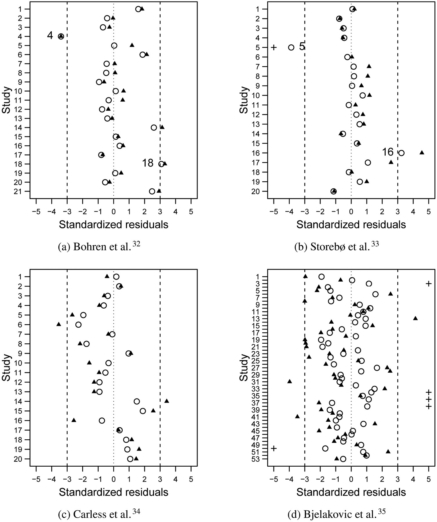
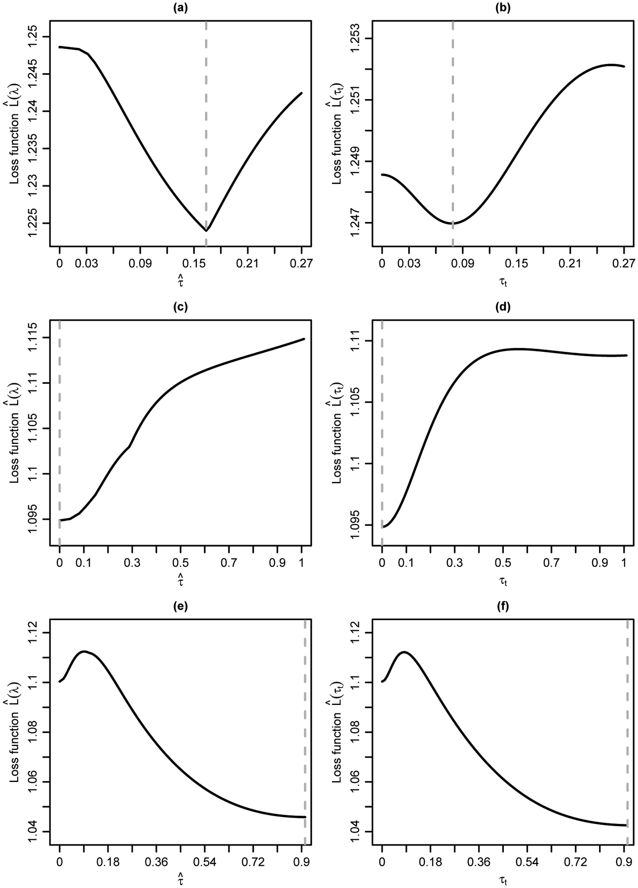
Figures 3(a)–3(c) show results of the penalization method by tuning λ. The transformation log(λ + 1) is used in these plots to better visualize the tuning parameter. In Figure 3(a), the estimated between-study SD $\widehat{\tau }$ shrinks toward 0 as λ increases. When λ is larger than a user-specified threshold, $\widehat{\tau }=0$. This trend is consistent with our theoretical results provided in Appendix A.1. Because there is a monotone relationship between λ and $\widehat{\tau }$ in this example, the loss function in terms of λ, shown in Figure 3(b), has a similar trend to that in terms of $\widehat{\tau }$ in Figure 3(c). The left/right tail of the loss function of λ is mapped to the right/left tail of $\widehat{\tau }$, with the optimal value of λ corresponding to that of $\widehat{\tau }$.

FIGURE 3.

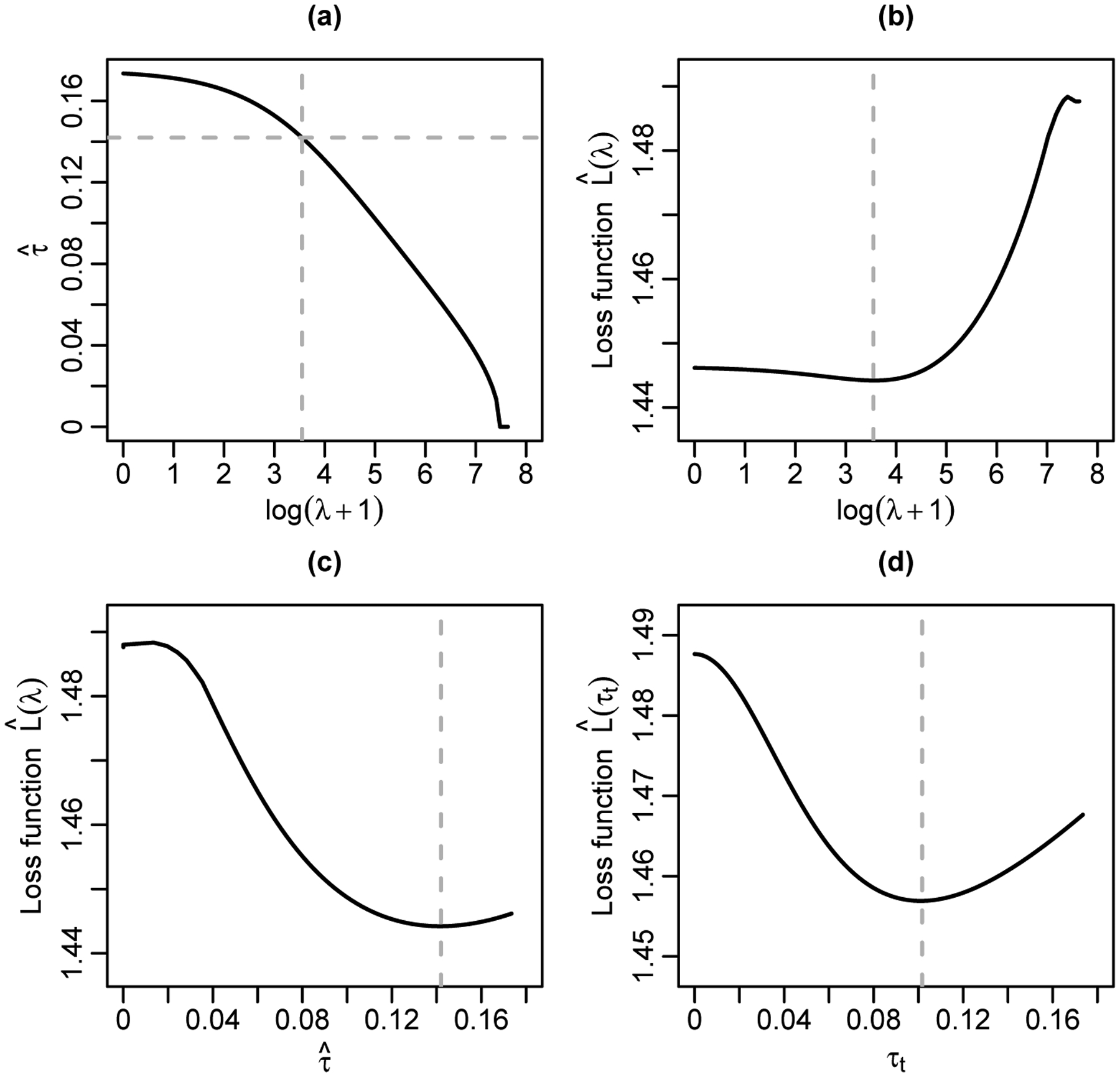
Illustration of the penalization methods using the meta-analysis by Bohren et al.³² (a) The estimated between-study standard deviation against the tuning parameter λ for the penalized likelihood. (b) The loss function against the tuning parameter λ. (c) The loss function against the estimated between-study standard deviation by tuning λ. (d) The loss function against the tuning parameter τ_t. Each vertical dashed line in panels (b)–(d) represents the optimal value that minimizes the loss function; the horizontal and vertical dashed lines in panel (a) correspond to the optimal values from panels (b) and (c).

Figure 3(d) shows the loss function by tuning τ. Compared with Figure 3(c), the loss function changes when tuning τ instead of λ, but the general trend is similar. As τ_t increases, the loss decreases to a minimum, followed by an increase. The optimal τ_t = 0.102, achieved by the loss function in Figure 3(d), is smaller than the estimated between-study SD of 0.142 that corresponds to the optimal λ when tuning λ in Figure 3(c).

4 |. SIMULATION STUDY

4.1 |. Simulation settings

We conducted a simulation study to compare the performance of the aforementioned approaches: the conventional CE and RE models; the penalization method by tuning λ; and the penalization method by tuning τ. Statistical performance was evaluated in terms of bias, mean squared error (MSE), and coverage probability of 95% CI. For each scenario described below, 5,000 replicates of meta-analyses were independently simulated.

The number of studies in each simulated meta-analysis was fixed as n = 30, and the within-study SE s_i was drawn from U(0.1, 1). Without loss of generality, the true overall effect size was μ = 0. The between-study SD was set to τ = 0, 0.5, 1, or 2. The true study-specific effect sizes were drawn from ${\mu }_i\stackrel{\text{ iid }}{~}N\left(\mu ,{\tau }^2\right)$, and the observed effect sizes were drawn from $y_i~N\left({\mu }_i,s_i^2\right)$.

Among the 30 studies in each simulated meta-analysis, m studies were modified to be outliers, and the number of outliers m was set to be 0, 1, …, or 6. Note that the marginal SD of y_i is $\sqrt{s_i^2+{\tau }^2}$ and the upper bound of $s_i^2$ was 1; we added a discrepancy of $3\sqrt{1^2+{\tau }^2}$ to those m studies, creating m outliers. With these seven choices of m, the proportion of outliers ranged from 0% to 20%. The penalization methods and the conventional CE and RE models were applied to each simulated meta-analysis to estimate the overall effect size and its 95% CI.

We additionally conducted more simulation studies to investigate the performance of the penalization methods under a broader range of settings, including meta-analyses with low to moderate heterogeneity but without outliers and meta-analyses with random effects following scaled t₅ distributions. See the details in Appendix B.

4.2 |. Simulation results

Table 1 presents the simulation results. When τ = 0 and m = 0, the CE model was the true model. In this scenario, the 95% CI coverage probability was fairly close to the nominal level, while all four methods produced the estimated overall effect size with nearly the same biases and MSEs. As m increased, due to the impact of the outlying studies, the CE model produced larger biases and MSEs than the RE model, as well as lower 95% CI coverage probabilities. The penalization methods, both by tuning λ and by tuning τ, performed better than the RE model with noticeably smaller biases and MSEs and higher 95% CI coverage probabilities. When τ = 0.5, each set of simulated studies in a meta-analysis were heterogeneous. As expected, in these instances, the RE model outperformed the CE model with respect to MSEs. When m was not large (e.g., 1 or 2), the RE model also slightly outperformed the penalization methods with smaller MSEs. As m increased, biases and MSEs produced by the penalization methods became smaller than those by the CE and RE models.

TABLE 1.

Biases, mean squared errors (MSEs), and 95% confidence interval coverage probabilities (CPs) in percentage for simulated meta-analyses using the four methods: common-effect model (CE); random-effects model (RE); penalization method for the random-effects model by tuning λ (PRE-λ); and penalization method for the random-effects model by tuning the between-study standard deviation (PRE-τ).

No. of outliers	CE			RE			PRE-λ			PRE-τ
	Bias	MSE	CP	Bias	MSE	CP	Bias	MSE	CP	Bias	MSE	CP
τ = 0:
0	0.001	0.004	95.1	0.002	0.004	95.7	0.001	0.004	95.9	0.001	0.004	95.8
1	0.103	0.040	70.2	0.081	0.015	95.7	0.064	0.011	97.2	0.077	0.015	96.0
2	0.205	0.094	45.8	0.184	0.045	90.4	0.149	0.036	95.7	0.176	0.045	92.0
3	0.309	0.169	25.9	0.294	0.098	77.2	0.244	0.081	89.8	0.272	0.092	84.5
4	0.409	0.259	13.2	0.399	0.170	54.2	0.345	0.147	80.2	0.361	0.154	76.2
5	0.507	0.365	5.8	0.501	0.262	28.7	0.451	0.237	68.9	0.459	0.241	67.2
6	0.608	0.493	2.3	0.603	0.374	10.3	0.557	0.349	59.5	0.561	0.350	58.5
τ = 0.5:
0	−0.003	0.031	49.9	−0.001	0.016	92.7	−0.002	0.020	94.2	−0.002	0.019	94.3
1	0.107	0.071	40.4	0.105	0.029	94.2	0.103	0.037	96.3	0.106	0.037	96.5
2	0.217	0.131	32.0	0.218	0.066	89.5	0.199	0.071	94.9	0.202	0.071	94.9
3	0.331	0.221	22.8	0.333	0.130	78.7	0.300	0.127	90.1	0.302	0.127	90.3
4	0.443	0.333	15.7	0.446	0.218	60.2	0.406	0.208	82.5	0.406	0.207	82.8
5	0.555	0.466	10.1	0.559	0.331	39.0	0.518	0.317	72.5	0.518	0.315	73.3
6	0.666	0.621	5.9	0.671	0.470	19.5	0.630	0.450	63.1	0.630	0.448	64.2
τ = 1:
0	−0.006	0.115	28.1	0.001	0.043	93.5	−0.002	0.057	96.5	−0.002	0.057	96.5
1	0.133	0.177	24.1	0.141	0.064	93.8	0.138	0.089	97.4	0.136	0.087	97.7
2	0.272	0.272	20.0	0.283	0.124	88.9	0.266	0.149	94.9	0.264	0.146	95.5
3	0.417	0.414	16.3	0.425	0.225	79.8	0.398	0.244	91.0	0.396	0.241	91.6
4	0.558	0.593	11.8	0.567	0.366	65.4	0.532	0.378	85.0	0.530	0.373	85.9
5	0.700	0.804	8.5	0.709	0.547	47.2	0.672	0.552	76.9	0.669	0.547	78.0
6	0.840	1.051	6.0	0.851	0.768	29.3	0.811	0.764	67.9	0.807	0.757	69.4
τ = 2:
0	−0.013	0.448	14.4	0.003	0.144	93.8	−0.001	0.207	97.3	−0.002	0.205	97.3
1	0.208	0.603	12.9	0.227	0.195	93.5	0.216	0.279	97.4	0.213	0.276	97.6
2	0.428	0.839	10.6	0.451	0.347	88.9	0.429	0.439	95.5	0.423	0.432	95.8
3	0.656	1.190	9.4	0.675	0.599	80.9	0.643	0.690	91.9	0.638	0.682	92.4
4	0.879	1.638	7.3	0.898	0.951	69.2	0.856	1.032	87.0	0.848	1.016	88.0
5	1.103	2.162	5.7	1.122	1.403	53.3	1.076	1.469	80.4	1.070	1.452	81.4
6	1.326	2.778	4.3	1.346	1.955	36.0	1.299	2.014	71.8	1.294	1.994	72.9

When the between-study heterogeneity was increased to τ = 1, the MSE produced by the RE model was generally smaller than those by the penalization methods. Nevertheless, the penalization methods generally outperformed both the CE and RE models with respect to biases and 95% CI coverage probabilities. When τ = 2 (i.e., substantial heterogeneity among the simulated studies within a meta-analysis), the CE model performed poorly; its MSEs were much larger than those for other methods, and its 95% CI coverage probabilities were roughly 10%. The RE model continued to have smaller MSEs than the penalization methods, possibly due to the variability of selecting the optimal tuning parameters when performing the penalization methods via the cross-validation procedure. Despite this, the coverage probabilities of the penalization methods were much higher than those for the RE model. Although biases and MSEs between the RE model and the penalization methods were close when τ and m were large (e.g., τ = 1, m = 6), subtle differences indicated that, compared with the RE model, the overall effect size estimates of the penalization methods were less biased and their SEs were larger. Therefore, the coverage probabilities of the penalization methods were noticeably higher than that of the RE model in all simulation scenarios. Results for the penalization methods by tuning λ were generally similar to those when tuning τ. Except when studies in the meta-analysis were truly homogeneous (i.e., τ = 0), tuning λ performed slightly better than tuning τ.

The penalization methods produced the estimated overall effect sizes with generally small biases and MSEs. This is due to the penalization methods incorporating features from both the CE and RE models by achieving a compromise between these two meta-analytic models. When τ was large, it dominated the discrepancies among studies, diminishing the impact of outlying studies. Consequently, the RE model might be favorable in such cases and generally produced smaller MSEs than the penalization methods. In addition, because the penalization methods used different weighting schemes than the CE and RE models, which reduced the influence of outliers on the variance of the estimated overall effect size, the respective 95% CI can be considered conservative, and its coverage probability was higher than those for both the CE and RE models.

5 |. EMPIRICAL DATA ANALYSES

We applied the proposed method to the four examples in Section 2 to further illustrate the real-world performance of the penalization methods. Because the performance of the penalization methods may depend on the between-study distribution in meta-analyses, we examined the normality assumption for the four examples; Appendix C presents the details. Table 2 presents the summary results of the four examples.

TABLE 2.

Summary results of the four examples.

Meta-analysis	No. of studies	I2 (95% CI)	No. of outliers		Overall effect size (95% CI)
			CE	RE	CE	RE	PRE-λ	PRE-τ
Bohren et al.32	21	57% (28%, 93%)	3	2	1.18 (1.09, 1.26)	1.33 (1.16, 1.52)	1.31 (1.14, 1.49)	1.27 (1.11, 1.46)
Storebø et al.33	20	73% (47%, 88%)	2	2	1.20 (1.11, 1.28)	1.29 (1.10, 1.51)	1.26 (1.07, 1.48)	1.22 (1.03, 1.44)
Carless et al.34	20	69% (58%, 92%)	2	0	0.46 (0.37, 0.58)	0.35 (0.20, 0.63)	0.46 (0.22, 0.98)	0.46 (0.22, 0.98)
Bjelakovic et al.35	53	96% (94%, 98%)	8	0	0.50 (0.48, 0.52)	0.31 (0.23, 0.42)	0.31 (0.23, 0.42)	0.31 (0.23, 0.42)

For the meta-analysis by Bohren et al.,³² the CE model estimated the overall OR as 1.18 with 95% CI (1.09, 1.26), and the RE model estimated it as 1.33 with 95% CI (1.16, 1.52) and ${\widehat{\tau }}_{\text{RE}}=0.17$. The I² statistic was 57% with 95% CI (28%, 93%),^46,39 implying moderate or substantial heterogeneity.^47,2 Figures 3(c) and 3(d) have shown loss functions for the penalization methods. Losses were minimized between 0 and ${\widehat{\tau }}_{\text{RE}}$, thus the penalization methods favored neither the CE nor RE models. When tuning λ, the overall OR estimate was 1.31 with 95% CI (1.14, 1.49). When tuning τ, the overall OR estimate was 1.27 with 95% CI (1.11, 1.46).

For the meta-analysis reported by Storebø et al.,³³ the CE model estimated the overall RR as 1.20 with 95% CI (1.11, 1.28), and the RE model estimated it as 1.29 with 95% CI (1.10, 1.51) and ${\widehat{\tau }}_{\text{RE}}=0.27$. The I² statistic was 73% with 95% CI (47%, 88%), indicating substantial heterogeneity. Figures 4(a) and 4(b) show the loss functions for the penalization methods by tuning λ and τ, respectively. Similar to the first example, losses were minimized between 0 and ${\widehat{\tau }}_{\text{RE}}$, and the penalization methods favored neither the CE nor RE models. When tuning λ, the overall RR was estimated as 1.26 with 95% CI (1.07, 1.48) and $\widehat{\tau }=0.16$. When tuning τ, the penalization for the between-study variance was heavier. The overall RR estimate was 1.22 with 95% CI (1.03, 1.44) and τ_t = 0.08.

FIGURE 4.

Loss functions for the meta-analyses by Storebø et al.³³ (upper panels), by Carless et al.³⁴ (middle panels), and by Bjelakovic et al.³⁵ (lower panels). The left panels show the loss functions by tuning λ against the estimated between-study standard deviation; the right panels show the loss functions by tuning τ against τ_t. Each vertical dashed line represents the optimal value that yields the minimum loss.

For the meta-analysis by Carless et al.,³⁴ the CE model yielded the estimated overall OR of 0.46 with 95% CI (0.37, 0.58). The RE model yielded a smaller OR estimate 0.35 with 95% CI (0.20, 0.63) and ${\widehat{\tau }}_{\text{RE}}=1.01$. The RE model seemed to be preferred based on Figure 2(c) because there were no outliers under the RE setting. However, Figures 4(c) and 4(d) present the loss functions of the penalization methods by tuning both λ and τ, respectively, where the minimum losses were achieved at $\widehat{\tau }=0$ and τ_t = 0, both corresponding to the CE model. These might not be consistent with the result of I² = 69% with 95% CI (58%, 92%), which implied substantial heterogeneity. The inconsistency was likely due to the impact of outlying studies on I².¹⁵ Additionally, the penalization methods estimated the overall OR as 0.46 with a 95% CI (0.22, 0.98). The point estimate was identical to the CE estimate because the optimal between-study SD used for weighting was 0. However, the 95% CI was wider than that of the CE model because the penalization methods incorporated the RE setting to construct the CI.

Last, for the meta-analysis by Bjelakovic et al.,³⁵ the CE model estimated the overall OR as 0.50 with 95% CI (0.48, 0.52), and the RE model estimated it as 0.31 with 95% CI (0.23, 0.42) and ${\widehat{\tau }}_{\text{RE}}=0.91$. The I² statistic was 96% with 95% CI (94%, 98%), indicating considerable heterogeneity. Figures 4(e) and 4(f) show loss functions. In contrary to the third example above, losses were minimized at ${\widehat{\tau }}_{\text{RE}}$ for both penalization methods, so the RE model was favored. The estimated overall ORs of the penalization methods were identical to that of the RE model, namely 0.31 with 95% CI (0.23, 0.42). This identical conclusion was consistent with the implication from Figure 2(d), where the CE setting led to many outliers but the RE setting did not lead to an outlier.

6 |. DISCUSSION

We have proposed penalization methods to estimate the overall effect size and its 95% CI in a meta-analysis. Simulation studies have shown that the penalization methods generally produced estimates with less biases and smaller MSEs and higher 95% CI coverage probabilities than the conventional CE and RE models in the presence of outliers. In practice, outliers frequently appear in meta-analyses and may have a substantial impact on meta-analytic results.¹⁵ It is inappropriate to simply remove outliers from meta-analyses without solid justification (e.g., evident errors and poor study designs), because such removal may lead to research waste and possible selection bias. The penalization methods provide a novel way to reduce the impact of outliers in meta-analyses by penalizing potentially overestimated heterogeneity and achieving a compromise between the CE and RE models.

Although Section 3.5 and the simulation results showed that the penalization method of tuning λ performs similarly to the penalization method of tuning τ, this may not always be true. When the tuning parameter is λ, from Equations (3) and (8), a single value of estimated τ may correspond to multiple loss values (e.g., all values of λ > λ_max lead to $\widehat{\tau }=0$, but they could have different loss values). Nevertheless, there is a deterministic relationship between τ_t and the corresponding loss from Equation (9). Appendix D provides two additional examples, in which different conclusions could be obtained by tuning different parameters. Specifically, in one example, tuning λ yields an estimate between the CE and RE estimates, while tuning τ yields the CE estimate. In another example, tuning λ yields the RE estimate, while tuning τ yields an estimate between the CE and RE estimates.

The penalization methods may have several limitations. First, they are motivated to deal with the issue when between-study heterogeneity is overestimated (e.g., due to outliers). However, the between-study heterogeneity can be underestimated in some cases. For example, in the presence of publication bias or small-study effects, studies with unfavorable results in a certain direction may be suppressed, leading to a narrower range of study results and thus underestimated heterogeneity compared to a “complete” set of studies.^48,49 As a future project, we may extend the penalization methods to handle this problem of underestimated heterogeneity by choosing the tuning parameter τ_t from a wider range of candidate values than [0, ${\widehat{\tau }}_{\text{RE}}$]. Second, the penalization methods were built on the ML estimation. The ML performance, however, has been shown to be slightly inferior to some alternative estimators.^39,40 The penalization methods may be extended to other estimation procedures, such as REML. It will be interesting to explore more robust heterogeneity estimators that could improve the penalization methods. Third, as in many conventional meta-analysis methods, this article treats within-study sample variances as fixed, known values, while they are subject to sampling error in practice and may affect meta-analytic results.⁵⁰ One option would be to extend the penalization methods using generalized linear mixed models for binary outcome measures.^51,52

In addition, this article has focused on the conventional univariate meta-analysis. However, advanced methods have been developed to simultaneously analyze multivariate outcomes and multiple treatments to improve the effect size estimates and allow indirect comparisons.^{53,54,55,56,57} The penalization methods may also be extended to multivariate meta-analyses by tuning the between-study variances of the multiple endpoints. Moreover, we developed the penalization methods under the framework of frequentist meta-analyses. From the Bayesian perspective, penalizing the between-study variance is equivalent to assigning a prior distribution to the variance component τ² or τ. Meta-analysts may use informative priors based on external evidence to aid the estimation of the between-study variance, which may be particularly helpful for meta-analyses with a relatively small number of studies.^58,59

References

- 1.Gurevitch J, Koricheva J, Nakagawa S, Stewart G Meta-analysis and the science of research synthesis. Nature. 2018;555(7695):175–182. [DOI] [PubMed] [Google Scholar]
- 2.Higgins JPT, Thomas J, Chandler J, et al. Cochrane Handbook for Systematic Reviews of Interventions. Chichester, UK: John Wiley & Sons; 2nd ed.2019. [Google Scholar]
- 3.Niforatos JD, Weaver M, Johansen ME Assessment of publication trends of systematic reviews and randomized clinical trials, 1995 to 2017. JAMA Internal Medicine. 2019;179(11):1593–1594. [DOI] [PMC free article] [PubMed] [Google Scholar]
- 4.Lin L, Chu H Meta-analysis of proportions using generalized linear mixed models. Epidemiology. 2020;31(5):713–717. [DOI] [PMC free article] [PubMed] [Google Scholar]
- 5.Bender R, Friede T, Koch A, et al. Methods for evidence synthesis in the case of very few studies. Research Synthesis Methods. 2018;9(3):382–392. [DOI] [PMC free article] [PubMed] [Google Scholar]
- 6.Borenstein M, Hedges LV, Higgins JPT, Rothstein HR A basic introduction to fixed-effect and random-effects models for meta-analysis. Research Synthesis Methods. 2010;1(2):97–111. [DOI] [PubMed] [Google Scholar]
- 7.Serghiou S, Goodman SN Random-effects meta-analysis: summarizing evidence with caveats. JAMA. 2019;321(3):301–302. [DOI] [PubMed] [Google Scholar]
- 8.Thompson SG Why sources of heterogeneity in meta-analysis should be investigated. BMJ. 1994;309(6965):1351–1355. [DOI] [PMC free article] [PubMed] [Google Scholar]
- 9.Spiegelman D, Khudyakov P, Wang M, Vanderweele TJ Evaluating public health interventions: 7. Let the subject matter choose the effect measure: ratio, difference, or something else entirely. American Journal of Public Health. 2018;108(1):73–76. [DOI] [PMC free article] [PubMed] [Google Scholar]
- 10.DerSimonian R, Laird N Meta-analysis in clinical trials. Controlled Clinical Trials. 1986;7(3):177–188. [DOI] [PubMed] [Google Scholar]
- 11.Whitehead A, Whitehead J A general parametric approach to the meta-analysis of randomized clinical trials. Statistics in Medicine. 1991;10(11):1665–1677. [DOI] [PubMed] [Google Scholar]
- 12.Takkouche B, Cadarso-Suarez C, Spiegelman D Evaluation of old and new tests of heterogeneity in epidemiologic meta-analysis. American Journal of Epidemiology. 1999;150(2):206–215. [DOI] [PubMed] [Google Scholar]
- 13.Higgins JPT, Thompson SG Quantifying heterogeneity in a meta-analysis. Statistics in Medicine. 2002;21(11):1539–1558. [DOI] [PubMed] [Google Scholar]
- 14.Lin L, Chu H, Hodges JS Alternative measures of between-study heterogeneity in meta-analysis: reducing the impact of outlying studies. Biometrics. 2017;73(1):156–166. [DOI] [PMC free article] [PubMed] [Google Scholar]
- 15.Ma X, Lin L, Qu Z, Zhu M, Chu H Performance of between-study heterogeneity measures in the Cochrane Library. Epidemiology. 2018;29(6):821–824. [DOI] [PMC free article] [PubMed] [Google Scholar]
- 16.Lin L Comparison of four heterogeneity measures for meta-analysis. Journal of Evaluation in Clinical Practice. 2020;26(1):376–384. [DOI] [PubMed] [Google Scholar]
- 17.Rücker G, Schwarzer G, Carpenter JR, Schumacher M Undue reliance on I2 in assessing heterogeneity may mislead. BMC Medical Research Methodology. 2008;8(1):79. [DOI] [PMC free article] [PubMed] [Google Scholar]
- 18.Takkouche B, Khudyakov P, Costa-Bouzas J, Spiegelman D Confidence intervals for heterogeneity measures in meta-analysis. American Journal of Epidemiology. 2013;178(6):993–1004. [DOI] [PMC free article] [PubMed] [Google Scholar]
- 19.Hoaglin DC Misunderstandings about Q and ‘Cochran’s Q test’ in meta-analysis. Statistics in Medicine. 2016;35(4):485–495. [DOI] [PubMed] [Google Scholar]
- 20.Borenstein M, Higgins JPT, Hedges LV, Rothstein HR Basics of meta-analysis: I2 is not an absolute measure of heterogeneity. Research Synthesis Methods. 2017;8(1):5–18. [DOI] [PubMed] [Google Scholar]
- 21.Higgins JPT, Thompson SG, Spiegelhalter DJ A re-evaluation of random-effects meta-analysis. Journal of the Royal Statistical Society: Series A (Statistics in Society). 2009;172(1):137–159. [DOI] [PMC free article] [PubMed] [Google Scholar]
- 22.Riley RD, Higgins JPT, Deeks JJ Interpretation of random effects meta-analyses. BMJ. 2011;342:d549. [DOI] [PubMed] [Google Scholar]
- 23.IntHout J, Ioannidis JPA, Rovers MM, Goeman JJ Plea for routinely presenting prediction intervals in meta-analysis. BMJ Open. 2016;6(7):e010247. [DOI] [PMC free article] [PubMed] [Google Scholar]
- 24.Lin L Use of prediction intervals in network meta-analysis. JAMA Network Open. 2019;2(8):e199735. [DOI] [PMC free article] [PubMed] [Google Scholar]
- 25.Hedges LV, Vevea JL Fixed- and random-effects models in meta-analysis. Psychological Methods. 1998;3(4):486–504. [Google Scholar]
- 26.Henmi M, Copas JB Confidence intervals for random effects meta-analysis and robustness to publication bias. Statistics in Medicine. 2010;29(29):2969–2983. [DOI] [PubMed] [Google Scholar]
- 27.Stanley TD, Doucouliagos H Neither fixed nor random: weighted least squares meta-analysis. Statistics in Medicine. 2015;34(13):2116–2127. [DOI] [PubMed] [Google Scholar]
- 28.Doi SAR, Barendregt JJ, Khan S, Thalib L, Williams GM Advances in the meta-analysis of heterogeneous clinical trials I: the inverse variance heterogeneity model. Contemporary Clinical Trials. 2015;45:130–138. [DOI] [PubMed] [Google Scholar]
- 29.Lin L, Aloe AM Evaluation of various estimators for standardized mean difference in meta-analysis. Statistics in Medicine. 2021;40(2):403–426. [DOI] [PMC free article] [PubMed] [Google Scholar]
- 30.Tibshirani R Regression shrinkage and selection via the lasso. Journal of the Royal Statistical Society. Series B (Methodological). 1996;58(1):267–288. [Google Scholar]
- 31.Heinze G, Wallisch C, Dunkler D Variable selection – a review and recommendations for the practicing statistician. Biometrical Journal. 2018;60(3):431–449. [DOI] [PMC free article] [PubMed] [Google Scholar]
- 32.Bohren MA, Hofmeyr GJ, Sakala C, Fukuzawa RK, Cuthbert A Continuous support for women during childbirth. Cochrane Database of Systematic Reviews. 2017;7:Art. No.: CD003766. [DOI] [PMC free article] [PubMed] [Google Scholar]
- 33.Storebø OJ, Ramstad E, Krogh HB, et al. Methylphenidate for children and adolescents with attention deficit hyperactivity disorder (ADHD). Cochrane Database of Systematic Reviews. 2015;11:Art. No.: CD009885. [DOI] [PMC free article] [PubMed] [Google Scholar]
- 34.Carless PA, Rubens FD, Anthony DM, O’Connell D, Henry DA Platelet-rich-plasmapheresis for minimising peri-operative allogeneic blood transfusion. Cochrane Database of Systematic Reviews. 2011;3:Art. No.: CD004172. [DOI] [PubMed] [Google Scholar]
- 35.Bjelakovic G, Gluud LL, Nikolova D, et al. Vitamin D supplementation for prevention of mortality in adults. Cochrane Database of Systematic Reviews. 2014;1:Art. No.: CD007470. [DOI] [PMC free article] [PubMed] [Google Scholar]
- 36.Hedges LV, Olkin I Statistical Method for Meta-Analysis. Orlando, FL: Academic Press; 1985. [Google Scholar]
- 37.Viechtbauer W, Cheung MWL Outlier and influence diagnostics for meta-analysis. Research Synthesis Methods. 2010;1(2):112–125. [DOI] [PubMed] [Google Scholar]
- 38.Cornell JE, Mulrow CD, Localio R, et al. Random-effects meta-analysis of inconsistent effects: a time for change. Annals of Internal Medicine. 2014;160(4):267–270. [DOI] [PubMed] [Google Scholar]
- 39.Veroniki AA, Jackson D, Viechtbauer W, et al. Methods to estimate the between-study variance and its uncertainty in meta-analysis. Research Synthesis Methods. 2016;7(1):55–79. [DOI] [PMC free article] [PubMed] [Google Scholar]
- 40.Langan D, Higgins JPT, Jackson D, et al. A comparison of heterogeneity variance estimators in simulated random-effects meta-analyses. Research Synthesis Methods. 2019;10(1):83–98. [DOI] [PubMed] [Google Scholar]
- 41.Normand SLT Meta-analysis: formulating, evaluating, combining, and reporting. Statistics in Medicine. 1999;18(3):321–359. [DOI] [PubMed] [Google Scholar]
- 42.Jackson D, Bowden J, Baker R How does the DerSimonian and Laird procedure for random effects meta-analysis compare with its more efficient but harder to compute counterparts?. Journal of Statistical Planning and Inference. 2010;140(4):961–970. [Google Scholar]
- 43.Bondell HD, Krishna A, Ghosh SK Joint variable selection for fixed and random effects in linear mixed-effects models. Biometrics. 2010;66(4):1069–1077. [DOI] [PMC free article] [PubMed] [Google Scholar]
- 44.Ibrahim JG, Zhu H, Garcia RI, Guo R Fixed and random effects selection in mixed effects models. Biometrics. 2011;67(2):495–503. [DOI] [PMC free article] [PubMed] [Google Scholar]
- 45.Cole SR, Chu H, Greenland S Maximum likelihood, profile likelihood, and penalized likelihood: a primer. American Journal of Epidemiology. 2014;179(2):252–260. [DOI] [PMC free article] [PubMed] [Google Scholar]
- 46.Viechtbauer W Confidence intervals for the amount of heterogeneity in meta-analysis. Statistics in Medicine. 2007;26(1):37–52. [DOI] [PubMed] [Google Scholar]
- 47.Higgins JPT, Thompson SG, Deeks JJ, Altman DG Measuring inconsistency in meta-analyses. BMJ. 2003;327(7414):557–560. [DOI] [PMC free article] [PubMed] [Google Scholar]
- 48.Turner EH, Matthews AM, Linardatos E, Tell RA, Rosenthal R Selective publication of antidepressant trials and its influence on apparent efficacy. New England Journal of Medicine. 2008;358(3):252–260. [DOI] [PubMed] [Google Scholar]
- 49.Lin L, Chu H Quantifying publication bias in meta-analysis. Biometrics. 2018;74(3):785–794. [DOI] [PMC free article] [PubMed] [Google Scholar]
- 50.Lin L Bias caused by sampling error in meta-analysis with small sample sizes. PLOS ONE. 2018;13(9):e0204056. [DOI] [PMC free article] [PubMed] [Google Scholar]
- 51.Chu H, Nie L, Chen Y, Huang Y, Sun W Bivariate random effects models for meta-analysis of comparative studies with binary outcomes: methods for the absolute risk difference and relative risk. Statistical Methods in Medical Research. 2012;21(6):621–633. [DOI] [PMC free article] [PubMed] [Google Scholar]
- 52.Jackson D, Law M, Stijnen T, Viechtbauer W, White IR A comparison of seven random-effects models for meta-analyses that estimate the summary odds ratio. Statistics in Medicine. 2018;37(7):1059–1085. [DOI] [PMC free article] [PubMed] [Google Scholar]
- 53.Ritz J, Demidenko E, Spiegelman D Multivariate meta-analysis for data consortia, individual patient meta-analysis, and pooling projects. Journal of Statistical Planning and Inference. 2008;138(7):1919–1933. [Google Scholar]
- 54.Jackson D, Riley R, White IR Multivariate meta-analysis: potential and promise. Statistics in Medicine. 2011;30(20):2481–2498. [DOI] [PMC free article] [PubMed] [Google Scholar]
- 55.Zhang J, Carlin BP, Neaton JD, et al. Network meta-analysis of randomized clinical trials: reporting the proper summaries. Clinical Trials. 2014;11(2):246–262. [DOI] [PMC free article] [PubMed] [Google Scholar]
- 56.Hong H, Chu H, Zhang J, Carlin BP A Bayesian missing data framework for generalized multiple outcome mixed treatment comparisons. Research synthesis methods. 2016;7(1):6–22. [DOI] [PMC free article] [PubMed] [Google Scholar]
- 57.Riley RD, Jackson D, Salanti G, et al. Multivariate and network meta-analysis of multiple outcomes and multiple treatments: rationale, concepts, and examples. BMJ. 2017;358:j3932. [DOI] [PMC free article] [PubMed] [Google Scholar]
- 58.Turner RM, Davey J, Clarke MJ, Thompson SG, Higgins JPT Predicting the extent of heterogeneity in meta-analysis, using empirical data from the Cochrane Database of Systematic Reviews. International Journal of Epidemiology. 2012;41(3):818–827. [DOI] [PMC free article] [PubMed] [Google Scholar]
- 59.Rosenberger KJ, Xing A, Murad MH, Chu H, Lin L Prior choices of between-study heterogeneity in contemporary Bayesian network meta-analyses: an empirical study. Journal of General Internal Medicine. 2021;36(4):1049–1057. [DOI] [PMC free article] [PubMed] [Google Scholar]
Associated Data
This section collects any data citations, data availability statements, or supplementary materials included in this article.