Abstract
Statistical shape modeling (SSM) is widely used in biology and medicine as a new generation of morphometric approaches for the quantitative analysis of anatomical shapes. Technological advancements of in vivo imaging have led to the development of open-source computational tools that automate the modeling of anatomical shapes and their population-level variability. However, little work has been done on the evaluation and validation of such tools in clinical applications that rely on morphometric quantifications. Here, we systematically assess the outcome of widely used, state-of-the-art SSM tools, namely ShapeWorks, Deformetrica, and SPHARM-PDM. We use both quantitative and qualitative metrics to evaluate shape models from different tools. We propose validation frameworks for anatomical landmark/measurement inference and lesion screening. We also present a lesion screening method to objectively characterize subtle abnormal shape changes with respect to learned population-level statistics of controls. Results demonstrate that SSM tools display different levels of consistencies, where ShapeWorks and Deformetrica models are more consistent compared to models from SPHARM-PDM due to the groupwise approach of estimating surface correspondences. Furthermore, ShapeWorks and Deformetrica shape models are found to capture clinically relevant population-level variability compared to SPHARM-PDM models.
Keywords: Statistical shape models, Population analysis, Correspondence optimization, Surface parameterization, Algorithm evaluation and validation, Landmark inference, Lesion screening
1. Introduction
Shape is the geometric information that remains when all the global geometrical properties are factored out, such as translation, orientation, and size (Mardia and Dryden, 1989). Since the pioneering work of D’Arcy Thompson (Thomson, 1917), morphometrics or shape analysis has evolved into an indispensable quantitative tool in medical and biological sciences to study shapes. Shape analysis has several applications in archaeology (Woods et al., 2017), medical imaging (Joskowicz, 2018; Heimann and Meinzer, 2009), computer-aided design (Joskowicz, 2018; Zadpoor and Weinans, 2015; Kozic et al., 2010), and biomechanics (Bredbenner et al., 2014; Nicolella and Bredbenner, 2012).
Statistical shape modeling (SSM) is the application of mathematics, statistics, and computing to parse the shape into some quantitative representation that will facilitate testing of biologically relevant hypotheses. SSM can help answer various questions about the population under study. Among the many examples, SSM can answer whether a specific bone can be used to classify a group of species in evolutionary biology (Dominguez and Crowder, 2012), how a gene mutation contributes to skeletal development (Twigg et al., 2009), the shape changes of brain structures in patients with depression and schizophrenia (Styner et al., 2006; Zhao et al., 2008; Davies et al., 2003), and the extent of bone deformation due to genetic diseases that can cause a specific type of cancer (Liu et al., 2015; Cates et al., 2017b). The quantitative, population-level analysis of anatomical shapes can also assist in different clinical applications, including disease diagnosis (Kohara et al., 2011), optimal implant design and selection (Goparaju et al., 2018), anatomy reconstruction and segmentation (Gollmer et al., 2014) from medical images for computer-aided surgery (Zachow, 2015), and preoperative and postoperative surgical planning (Rodriguez-Florez et al., 2017; Markelj et al., 2012; Zheng et al., 2009). These advancements in biomedical and clinical applications that benefit from SSM have the potential to make clinical-decision making more objective.
Computational tools for shape modeling define an anatomical mapping among shapes to enable quantifying subtle shape differences and performing shape statistics. That is, the shapes that differ in a manner that is typical of the shape variability in the population are considered similar compared to the shapes that differ in atypical ways. For example, extra bone growth on a femur that is indicative of a pathology differs from a control femur in an atypical way. A growing consensus in the field is that such a metric should be adapted to the specific population under investigation, which entails finding correspondences across an ensemble of shapes (Srivastava et al., 2005; Kulis et al., 2013). Manually defined landmarks, defined consistently on each shape instance have been the most popular choice for a light-weight shape representation that is suitable for statistical analysis and visual communication of the results (Zachow, 2015; Sarkalkan et al., 2014). However, manual annotation is tedious, time-consuming, and expert-driven (hence subjective). Manual annotation is prohibitive for three-dimensional (3D) shapes, especially with large shape ensembles. SSM is an important shift from manually defined anatomical homologies to computationally derived correspondence shape models. Finding correspondences across an ensemble of shapes can be posed as an optimization problem leading to the development of various open-source SSM tools.
The scientific premise of existing correspondence techniques falls in two broad categories, pairwise and groupwise (Oguz et al., 2015). The pairwise approach treats each shape instance independently and estimates correspondences by mapping the subject to a predefined atlas or template (e.g., SPHARM-PDM (Styner et al., 2006)). The groupwise approach, on the other hand, estimates point correspondences by considering the variability in the entire cohort of shapes to quantify the quality of correspondences (e.g., ShapeWorks (Cates et al., 2017a), Minimum Description Length - MDL (Davies, 2002), Deformetrica (Durrleman et al., 2014)). Hence, groupwise methods learn a population-specific metric in a way that does not penalize natural variability and therefore can capture the underlying parameters in an anatomical shape space. Other publicly available tools, e.g., FreeSurfer (Fischl et al., 1999), Brain Voyager (Goebel et al., 2006), FSL (Jenkinson et al., 2012), and SPM (Ashburner and John, 2012), provide shape modeling capabilities, but they are tailored to specific anatomies or limited topologies. Shape analysis tools, such as R shapes package (Dryden, 2018) and MorphoJ (Klingenberg, 2011), require point correspondences, defined manually or automatically via an SSM tool, for the input shapes to perform statistical analysis.
Better understanding of the consequences of different SSM tools for the final analysis is critical for the careful choice of the tool to be deployed for a clinical application. This study is thus motivated by the potential role of SSM in clinical scenarios that (1) are driven by anatomical measurements, which could be automated by relating patient-level anatomy to population-level morphometrics, and (2) entail pathology screening, which could be informed by population-level statistics of controls. In this paper, we significantly extend the preliminary analysis presented in (Goparaju et al., 2018) to expand the clinical application under analysis. In particular, we demonstrate the significance of evaluation and validation of SSM tools in the context of clinical applications, such as implant design and selection, motion tracking, surgical planning, and screening of bony lesions. Here, we consider a representative set of open-source, widely used SSM tools that support shape modeling of general anatomies; namely ShapeWorks (Cates et al., 2017a), Deformetrica (Durrleman et al., 2014), and SPHARM-PDM (Styner et al., 2006) (recently incorporated into SlicerSALT (Vicory et al., 2018)). We propose evaluation and validation frameworks for anatomical landmark/measurement inference and lesion screening. We also present a lesion screening method to provide an objective characterization of subtle abnormal shape changes with respect to learned population-level statistics of controls.
2. Related work
Open-source SSM tools rely on different modeling approaches and assumptions to establish surface correspondences. However, evaluating shape models is a nontrivial task due to the lack of ground-truth correspondences. Shape models can be intrinsically evaluated using quantitative metrics that reflect the correspondence quality (Davies, 2002). However, such metrics have been criticized since relevant shape information may be lost while still obtaining excellent evaluation measures (Ericsson and Karlsson, 2007). Hence, there is an unmet need to benchmark SSM tools via extrinsic validation metrics that signify the impact of shape models in clinical applications.
(Ericsson and Karlsson, 2007) relied on manually picked landmarks to validate the computationally derived correspondences. (Munsell et al., 2008) developed a similar approach to benchmark correspondence optimization techniques using synthetic shapes. These two approaches require ground-truth correspondences to evaluate shape models, which is not trivial, and is instead prohibitive, for non-synthetic 3D shapes (e.g., anatomies). Furthermore, (Munsell et al., 2008) conducted experiments for 2D shapes. Extending these techniques to 3D shapes would not be feasible, given the complexity of medical and biological shapes. These evaluation studies have theoretical grounds, yet have not considered real-world applications.
Very few studies have evaluated SSM tools in the context of biomedical applications. SSM tools have been evaluated in nonclinical applications such as image segmentation to quantify the influence of a shape model on the image segmentation accuracy (Gollmer et al., 2014). (Gao et al., 2014) proposed a framework for the generation of synthetic, ground-truth correspondences via a shape-deformation synthesis approach to compare shape models from SPHARM-MAT, SPHARM-PDM, ShapeWorks, and tensor-based morphometry (TBM). This study focused on shapes with simple geometric complexity and simulated pathologies. The comparison of the shape models found inconsistencies and disagreement among the different tools. However, little work has been done in the evaluation and validation of SSM tools in clinical applications. Hence, a systematic evaluation and validation framework that enables assessment of shape models from different tools can assist in SSM tool selection in clinical scenarios.
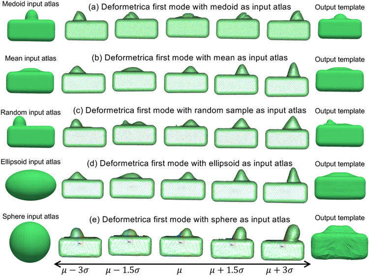
To demonstrate the need for and significance of SSM tool assessment, we performed a proof-of-concept experiment on an ensemble of 3D shapes of boxes with a moving bump, where computationally derived point correspondences were obtained using ShapeWorks (Cates et al., 2017a), Deformetrica (Durrleman et al., 2014), and SPHARM-PDM (Styner et al., 2006). This example is interesting because we would, in principle, expect an SSM tool to discover a single mode of variability, which is the moving bump, by generating surface correspondences that respect the natural shape variability in the population. However, different tools have yielded different results (Goparaju et al., 2018). ShapeWorks (Cates et al., 2017a), which adopts a groupwise approach, correctly discovered the underlying population variability and generated shape more faithful to those described by the training set, even out to three standard deviations. This proof-of-concept motivates the need to perform a systematic evaluation and validation of these SSM tools as related to application-specific clinical needs.
3. Background
Here, we give an overview of the SSM tools considered for the performance analysis and provide the clinical scenarios that can benefit from such analysis.
3.1. Statistical shape modeling (SSM) tools
A shape model provides both a detailed 3D geometrical representation of the average anatomy of a given population and a representation of the population-level geometric variability of the anatomy, in the form of a collection of principal modes of variation. SSM tools for point-based models automate the point-correspondence estimation of an ensemble of shapes via an optimization problem that quantifies the notion of correspondences. Once correspondences are obtained in a common coordinate system where rigid or similarity transformations are factored out, principal component analysis (PCA) can be performed to identify the dominant modes of variation in the shape space. Here, we overview the shape modeling approach pertaining to each of the considered SSM tools.
3.1.1. ShapeWorks
ShapeWorks is a groupwise particle-based shape modeling (PSM) method (Cates et al., 2017a, 2007) that is not constrained to any specific topology, handles open surfaces, and does not rely on any surface parameterizations. The PSM formulation details can be found in Appendix A.1. The scientific and clinical utility of ShapeWorks has been demonstrated in a range of applications, including neuroscience (Datar et al., 2013; Oguz et al., 2009), biological phenotyping (Jones et al., 2013; Cates et al., 2017b), orthopaedics (Harris et al., 2013; Jacxsens et al., 2019; Atkins et al., 2017b), and cardiology (Bieging et al., 2018b,a).
3.1.2. Deformetrica
Deformetrica is a groupwise correspondence method that is based on the large deformation diffeomorphic metric mapping (LDDMM) framework (Durrleman et al., 2014). This SSM tool is not constrained to any specific topology and supports open surfaces, but it requires an initial atlas that defines the topology of the shape class under study to estimate the template complex . Correspondences are not explicitly optimized; rather diffeomorphic deformations enable the correspondence establishment between the template complex and each input shape. The template complex captures the common characteristics of the shapes, and the deformations capture the variability in the shapes, as shown in Fig. 1(b). The technical details of Deformetrica can be found in Appendix A.2. Applications of Deformetrica include quantitative assessment of craniofacial surgery (Rodriguez-Florez et al.), classification of patients with Alzheimers disease (Routier et al., 2014), and cranioplasty surgical planning (Rodriguez-Florez et al., 2017).
Fig. 1.
SSM tools: (a) Shapeworks (Cates et al., 2017a) considers two random variables defining the configuration space and shape space. The configuration is a collection of M point correspondences on a shape, which is mapped to a single point in the dM–dimensional shape space; (b) Deformetrica (Durrleman et al., 2014) estimates a template from the set of input shapes and an initial atlas by generating point correspondences on the input shapes based on deformations; and (c) SPHARM-PDM (Styner et al., 2006) maps each input shape to a unit sphere through an area-preserving and distortion-minimizing objective using spherical harmonic basis functions, where color indicates correspondences between the sphere and the individual samples.
3.1.3. SPHARM-PDM
SPHARM-PDM is a pairwise parameterization-based correspondence method (Styner et al., 2006) that is restricted to anatomies with spherical topologies. The spherical parameterization is obtained by mapping each shape to a unit sphere through an area-preserving and distortion-minimizing objective using spherical harmonic (SPHARM) basis functions, as shown in Fig. 1(c). The SPHARM description is obtained from the surface mesh and its spherical parameterization, which are then aligned using a first-order ellipsoid from the SPHARM coefficients to establish correspondences across shapes. The technical details of SPHARM-PDM can be found in Appendix A.3. Applications of SPHARM-PDM include boundary and medical shape analysis of the hippocampus in schizophrenia (Styner et al., 2004), orthognathic surgical displacement analysis (Paniagua et al., 2011), and quantification of temporomandibular joint osteoarthritis.
3.2. Clinical applications
Clinical applications, such as implant design and selection, surgical planning, bone resection, and bone grafting, require patient-specific anatomical representation, which can be automatically estimated by relating patient-specific anatomical shape to the learned population-level morphometrics. Such automation reduces manual and subjective clinical decisions (Kohara et al., 2011; Rodriguez-Florez et al., 2017). In this paper, we consider a representative set of clinical needs that would benefit from SSM-informed decisions.
3.2.1. Implant design and selection – LAA closure
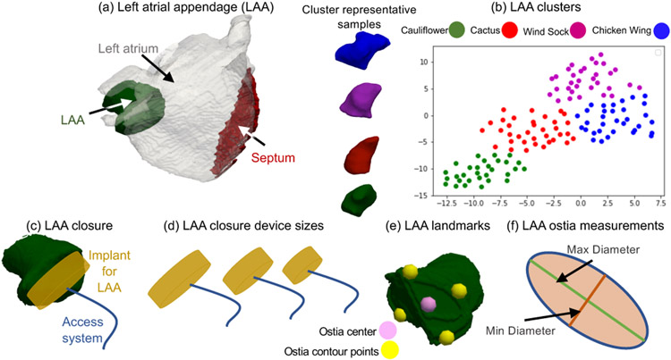
The left atrial appendage (LAA) is a small sack-like structure in the human heart. In atrial fibrillation (AF) patients, blood clots can form due to irregular heartbeat . LAA can be one of the sources for thrombus formation and may be responsible in circulating the blood clots through the body, causing stroke in AF patients (Regazzoli et al., 2015). To reduce the risk of stroke, clinicians occlude the appendage using a closure device (i.e., an implant) (Fig. 2(a)) (Regazzoli et al., 2015). LAA morphology is complex and categorized into four types (Wang et al., 2010): cauliflower, chicken wing, wind sock, and cactus (Fig. 2(b)), and hence closure implants are available in various sizes (Fig. 2(d)) (Romero et al., 2014). A clinician typically selects an appropriate device size by examining the patient-specific LAA morphology (Wang et al., 2010). Nonetheless, such examination entails significant manual effort for marking relevant anatomical landmarks and measurements, and thereby could lead to subjective and error-prone decisions. Inappropriate device selection would lead to an incomplete LAA closure that is worse than no closure (Regazzoli et al., 2015). SSM could thus provide an automated approach for developing less subjective categorizations of LAA morphology and anatomical measurements that can be used for more objective clinical decisions regarding suitability for LAA closure. SSM could further assist in designing more accurate, representative implant sizes for different LAA morphologies.
Fig. 2.
LAA Anatomy. (a) LAA is a sack-like structure in the human heart; (b) LAA morphology is categorized into four types: chicken wing, wind sock, cactus, and cauliflower (Wang et al., 2010). A 2D projection of the clustered LAA shapes from signed distance transform images using t-distributed stochastic neighbor embedding (t-SNE); (c) LAA closure is performed using an implant device through interatrial septum using an access system; (d) LAA closure device sizes available; (e) LAA ostia landmarks estimated to measure LAA ostia; and (f) LAA ostia measurements computed from the landmarks by fitting an ellipse.
3.2.2. Surgical planning – Total shoulder arthroplasty
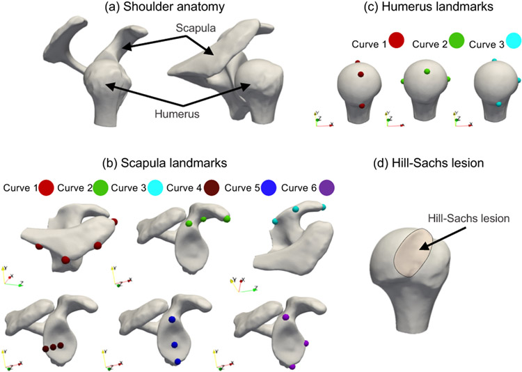
The scapula is part of the shoulder girdle and has shallow concave glenoid upon which the quasi-spherical humeral head articulates (Fig. 3(a)). The glenohumeral joint can be impaired and worn as seen in osteoarthritis. In these cases, joint replacement with a prosthetic implant, the anatomic total shoulder arthroplasty (aTSA), can reduce pain and restore the normal function of the shoulder joint. In aTSA, restoration of the glenohumeral joint to a nonpathologic state aims to obtain balanced forces on the glenoid and prosthetic components to maintain joint stability and improve the overall shoulder function. Because of the large anatomic variability of the glenoid (De Wilde et al., 2010), no consensus exists on which anatomical references should be used intraoperatively to restore the native glenoid. The inferior section of the glenoid has been found to be the most consistent, and was therefore proposed as a reference. The landmarks defining the native glenoid (Fig. 3(b) bottom row) are manually defined on the glenoid and are expert-driven, and thereby their identification can be subjective and error-prone. A patient-specific landmark inference of the scapula can be automated using SSM by relating subject-specific metrics to population-level metrics. Hence, SSM could assist in the restoration of the glenoid plane by providing an objective, automated solution for estimation of landmarks.
Fig. 3.
The human shoulder in SSM applications. (a) The cup-like glenoid of the scapula is the articulating surface for the ball-like humeral head; (b) scapula landmarks obtained for six curves for landmarks inference; (c) humerus landmarks obtained for three curves for landmarks inference; and (d) A Hill-Sachs lesion is formed in the humeral head via compression against the glenoid rim during a shoulder dislocation.
3.2.3. Surgical planning – Reverse total shoulder arthroplasty
Reverse shoulder arthroplasty is a good treatment option in shoulder pathology with dysfunction of the rotator cuff muscles (Saltzman et al., 2010), including cuff tear arthropathy, irreparable cuff tears, or proximal humerus fractures. In this surgical process, the ball-like structure (i.e., humerus) and socket-like structure (i.e., scapula) are interchanged, hence reversing the anatomy of the shoulder. By distalizing and medializing the glenohumeral center of rotation (COR), the lever arm of the deltoid muscle is increased so that it can take over shoulder function from the deficient rotator cuff. Lateralization of the humerus without changing the COR can also optimize muscle tension. On the other hand, too much COR lateralization or distalization can lead to bony impingement between the humerus and scapula, nerve lesions, or stress fractures of the scapula. This interplay amongst range of motion, implant stability, and avoidance of complications is determined by the design of the implant and the clinicians expertise. SSM could thus automate the inference of optimal COR and landmarks of the humerus to assist in better implant design and implant configuration selection. Furthermore, SSM could also improve the surgical process by objectively characterizing patient-level variability.
3.2.4. Bone grafting – Hill-Sachs lesion
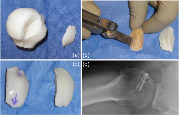
In cases of shoulder dislocation, the humeral head slips out of the shoulder socket and becomes compressed against the rim of the glenoid, which may lead to compression fractures on the humeral head, also known as a Hill-Sachs lesion (Fig. 3(d)). Large Hill-Sachs lesions have a high risk of recurrent shoulder instability, leading to impaired shoulder function and debilitating pain (Provencher et al., 2012). In cases of large Hills-Sachs lesions, bone grafting of the lesion has been suggested as a viable treatment option. The lesion characteristics are typically evaluated preoperatively on 2D CT-scans. During surgery, measurements are reevaluated using a ruler to choose the fresh frozen allograft that best fits into the defect. Translating this information into a 3D printed model (Fig. 4(a)) provides the surgeon with a hands-on template with which to properly template the allograft. Cuts on the allograft are made to shape the graft until it fits the lesion properly (Fig. 4(b)). This entire process is performed by trial and error and can vary based on the expertise of the clinician. SSM could assist in the systematic evaluation of the lesion, the lesion depth, and the objective characterization of the filling void to enable objective decisions for sizing and shaping the bone graft.
Fig. 4.
Hill-Sachs bone grafting. (a) A 3D printed model of a humeral head with a Hill-Sachs defect and a 3D model of the missing bone that fills the void; (b) Shaping a bony allograft to match the size, shape, and orientation of the 3D model; (c) The final graft (left) compared with the 3D template (right); and (d) Postoperative radiograph of the graft in the shoulder.
3.2.5. Bone resection - cam-type FAI lesion
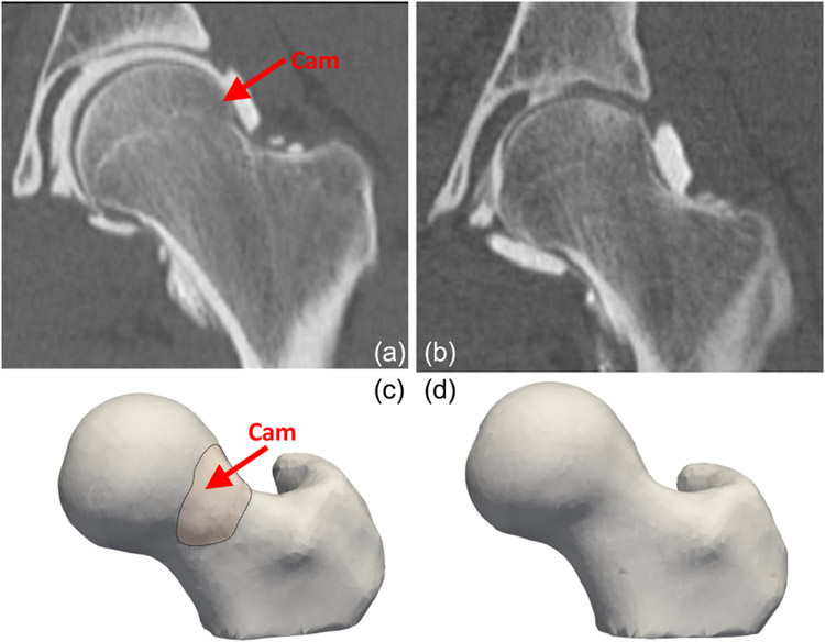
The hip is a ball-socket joint, with the femoral head acting as a ball, and the acetabulum, a component of the pelvis bone, acting as the socket. Femoroacetabular impingement (FAI) occurs when there is extra bone growth along one or both of the bones that form the hip joint (Fig. 5(a)), which thereby hampers smooth movement. Over time, this abnormal contact can cause damage to the labrum, which is a fibrocartilagenous tissue structure that surrounds the bony rim of the acetabulum. Patients with lesions on the femoral head and head-neck junction are diagnosed with cam-type FAI. Cam is a specific type of FAI in which the bone growth occurs to the femoral neck This lesion reduces the clearance between the femur and the pelvis since the femoral head does not remain round due to a formed bump (Fig. 5(c)). Cam-type morphology is believed to cause abnormal motion; notably, rotation of an aspherical femoral head within a relatively spherical socket likely causes the femur to lever-out, in turn leading to high shear stresses on cartilage and the acetabular labrum, leading to tears, fibrillation, and chronic inflammation. In cam-type FAI patients, the extra bone growth is removed through a surgical resection. Underestimating the resection depth can lead to revision surgery, whereas overestimating the resection depth can lead to hip fractures. Clinicians estimate the cam lesion and the resection depth through inspection of 2D radiographs and visual inspection at the time of surgery. However, these approaches are only semiquantitative, and may result in over or underestimation of the areal extent and magnitude of the deformity. SSM can automate the detection of the lesion and resection depth, resulting in fewer cases of revision hip arthroscopy.
Fig. 5.
Cam-type FAI lesion. (a) A CT scan of cam-type FAI femur (an extra bone growth on the femoral head); (b) A CT scan of a control femur; (c) A 3D segmented and preprocessed femur shape having cam-type FAI; and (d) A 3D segmented and preprocessed control femur.
4. Methods: Evaluating and validating SSM tools
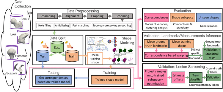
The assessment of an SSM tool is a multifaceted process where no single metric captures all performance aspects of the resulting shape models. Hence, we present systematic evaluation and validation frameworks (Fig. 6) to assess the point correspondences obtained from different SSM tools. The evaluation framework intrinsically assesses the quality of the shape model when the ground-truth correspondences are unavailable. The validation framework, on the other hand, is performed in the context of clinical applications where some ground-truth information, extrinsic to the shape model, is available. These frameworks can be applied to any SSM tool, beyond those considered here in this paper.
Fig. 6.
SSM evaluation and validation frameworks
4.1. Evaluation and validation frameworks: common steps
The common steps in the proposed evaluation and validation frameworks are as follows: (1) data collection; (2) data preprocessing; (3) data split; and (4) shape modeling. The data collection step entails segmenting anatomies-of-interest from the population under study and saving them as binary images for statistical analysis.
The data preprocessing step includes the following: closing small holes in the given segmentations; resampling volumes to have isotropic voxel spacing; antialiasing to remove the staircase effect on the image contours due to discretization (Whitaker, 2000); aligning center of mass; rigidly aligning shapes using the ensemble mediod as a reference and the advanced normalization tools (ANTs) (Avants et al., 2014) for registration; cropping using the largest bounding box that encapsulates all shape samples to remove the unnecessary background that can slow down the correspondence estimation; fast marching to convert segmentations to signed distance transforms; and topology-preserving smoothing. The preprocessed segmentations are then converted to the appropriate data type needed for each SSM tool.
The rigid registration step factors out only rotational and translational variations across the training samples, which are global geometric information that is not relevant to the shape modeling task. The reference shape for the rigid alignment was selected as a representative shape of the given shape ensemble using K-medoids clustering, assuming the ensemble belongs to one single cluster. Hence, the reference shape can be considered as the closest training sample to the average/mean shape of the ensemble. If registration is not performed prior to the shape modeling step, the resulting shape model would capture alignment differences as shape modes of variation and could dominate and hide the true factors of variations. Furthermore, training objectives for optimizing groupwise correspondences might not converge to useful population statistics. Different anatomies require different pre-alignment strategies. The goal is to remove misalignment prior to generating a correspondence model, but what that alignment is, depends on the data and the clinical application of interest.
The data split step involves creating training and test subsets. The training samples are used to train the shape model, and the testing samples are used for validation. Here, we use importance sampling to determine the training/testing splits, where a dataset is clustered and training/testing samples are selected from each cluster. The advantages of importance sampling are threefold. It obtains a sample population that best represents the entire population being studied, ensuring that each subgroup of interest is represented in the training dataset. It avoids too many experiments using cross-validation or bootstrapping, which are prohibitively expensive given the extent of analysis involved in this study. It also provides representative and viable comparisons across SSM tools in scenarios where the domain shift between training and testing data is minimal. However, the use of importance sampling could result in an optimistic estimation of the shape model performance. Hence, the presented results should not be considered as a baseline for the SSM tools in arbitrary training/testing scenarios.
Importance sampling is performed as a way of generating stratified samples. To this end, K-medoids clustering is performed to determine the training data. The input images to the k-medoids algorithm are signed distance transforms that are obtained from the data preprocessing step using fast marching. The k-medoids algorithm uses the squared Euclidean distance metric and the k-means++ (Arthur and Vassilvitskii, 2006) algorithm for choosing the initial mediod for each cluster. The choice of the number of clusters is the same for all datasets except for the LAA dataset. Based on the existing literature about the inherent clusters of the LAA morphology (Wang et al., 2010), we use 4 clusters of LAA and then randomly draw training and testing samples from each cluster based on the required percentage for the training/testing split. For the other datasets, we determined the number of clusters based on the percentage of the training samples we need. For example, if we need K samples of training data, k-medoids algorithm is run on the entire dataset with K clusters. If the training data consists of only controls, then only controls are provided as input to the k-medoids algorithm. The medoid of each cluster is then used as a training sample.
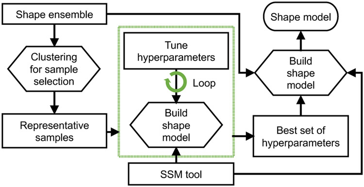
The shape modeling step estimates surface correspondences across the training samples using different SSM tools. Each tool (in particular, ShapeWorks and Deformetrica) has a set of algorithmic hyperparameters that need tuning. The hyperparameter tuning is performed on a representative subset of the training samples using K-mediods (Fig. 7). Evaluating the shape models with different sets of hyperparameters for the entire training data can easily become a prohibitively expensive and time-consuming process. Based on our experience with the SSM tools, not all hyperparameters can equally influence the resulting shape model. Hence, we considered those that typically impact the optimized shape models and used different combinations of these hyperparameters to build shape models for rapid evaluations. The tuning process is automated using bash scripts. This process is not needed for SPHARM because it follows a pairwise approach in generating point correspondences. The settings for SPHARM-PDM tool are the maximal degree for the SPHARM computation (spharmDegree) and the subdivision level for the icosahedron subdivisions (subdivLevel). subdivLevel of 10 and spharmDegree of 15 have been used to generate all the shape models. The models resulting from different hyperparameters parameters are compared qualitatively based on two criteria (since ground-truth correspondences are unavailable): (a) correspondence points are evenly spaced to cover the entire geometry; and (b) points are in good correspondence across the training data by inspecting their neighboring correspondences. The best set of hyperparameters is then used for training the shape model on the entire training subset. The trained shape models from SSM tools are used for both evaluation and validation.
Fig. 7.
Hyperparameters tuning. A representative subset is selected using clustering to generate the shape model in an efficient manner.
4.2. SSM evaluation
We use quantitative and qualitative metrics to evaluate shape models when ground-truth correspondences are not available.
4.2.1. Quantitative evaluation metrics
We adopt the quantitative metrics of compactness, generalization, and specificity (Davies et al., 2002) to assess different aspects of a shape model. These measures are functions of the number of modes of variation K ∈ {1,..., min(N, dM)} that are computed by PCA on correspondences, where N is the number of training shapes, d is the dimension of the configuration space, and M is the number of correspondences.
Compactness.
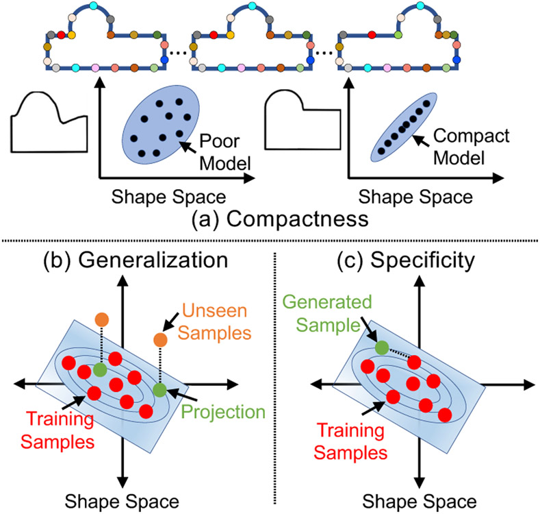
Although high-dimensional, the shape space can be parameterized by a low-dimensional subspace (defined by eigenvectors and associated eigenvalues) that explains the shape variability. A compactness measure echoes the Occam’s razor principle; “a simple explanation is more likely to be better than a complicated explanation.” Compactness can be computed as (Munsell et al., 2008), where K indicates the number of eigenvectors to explain the shape variability, and λj indicates the eigenvalue of the j–th mode. A compact shape model can thus explain a specific level of explained shape variance with fewer modes of variation, and the more compact a model is, the better (Fig. 8(a)).
Fig. 8.
Quantitative evaluation metrics. (a) A good shape model can encode the shape variability with fewer degrees of freedom; (b) a good shape model can spread between and around the training shapes to represent the unseen shapes; (c) a good shape model can generate plausible shapes.
Generalization
quantifies whether the probability density function learned by the shape model is able to spread between and around the given training shapes (Fig. 8(b)). We compute the generalization metric, denoted as G(K), using the left-out testing samples as follows: Consider a testing shape vector, , where n ∈ {1, …, Nts} and Nts is the number of testing samples, and a shape model that is obtained from the training shape vectors. Generalization can thus be quantified as , where εn(K) = ∥zn(K) − zn∥2 is the approximation error using the squared Euclidean distance when using the first K eigenvectors to represent the left-out shape instance. The generalization metric is monotonically decreasing with respect to the number of modes considered, provided the modes are of decreasing dominance. With more modes considered, the degrees of freedom of a shape model increase, and hence the capacity of the shape model increases. Thereby, the reconstructed samples will be more closer to the ground truth. A generalizable shape model can thus represent unseen shapes with a given level of error tolerance using fewer modes of variation.
Specificity
is the ability of the shape model to generate new, but valid, instances of shapes by constraining the variability in the shape space such that only legal/plausible shapes can be generated (Fig. 8(c)). Specificity can be quantified by randomly generating J (a large number of) samples z(K) from the shape space using the first K eigenvectors and eigenvalues, assuming a multivariate normal distribution, and computing the Euclidean distance to the closest training sample z′. Specificity is computed as (Munsell et al., 2008). The specificity metric is monotonically increasing with respect to the number of modes considered due to the increased intrinsic dimensionality of the shape space, where the expected distance between two shape samples is, with high probability, approximately twice the space dimensionality. Thereby, the generated samples tend to be farther away from the training data with the increased number of modes. A specific shape model can thus generate realistic shape samples within a given distance to training samples using fewer modes of variation.
It is worth noting that these metrics assume a multivariate Gaussian shape model, which is parameterized using PCA. PCA assumes linear correlations, and hence a very compact non-linear shape model might appear less compact through the lens of PCA. However, the specificity of such model will be penalized (i.e., higher values), since the assumed Gaussian model would generate shape samples from high-density regions in the shape space that are not faithful to the underlying shape distribution. Hence, these evaluation metrics should not be considered in isolation. To further justify the use of PCA for compactness evaluation, we conducted normality tests for all the shape models produced by the three SSM tools (see Appendix D for more details.) Furthermore, we computed compactness using kernel PCA to capture nonlinearities for all the shape models produced by the three SSM tools. We computed the compactness using the eigenvalue decomposition of the centralized kernel matrix. We did not observe significant changes in the compactness curves compared to using PCA (see Appendix E for more details).
4.2.2. Qualitative evaluation metrics
The qualitative assessment of shape models is performed using modes of variation and cluster analysis. The modes of variation may reflect clinically relevant variations/patterns. For instance, the anterior-posterior dilation of the left atrium shape is found to be statistically correlated with the severity of atrial fibrillation (Cates et al., 2014). Clustering is an approach to find groups in a population that are as distant as possible while ensuring the samples within a given group to be as similar as possible. Shape populations under analysis in clinical applications may exhibit natural clusters, different levels of illness, and disease progression. For instance, clustering analysis of the left atrium with different pulmonary veins branching might reveal clusters linked to atrial fibrillation pathology (Cates et al., 2014). A shape model is assessed by the ability to discover such hidden patterns in the shape class of interest.
Modes of variation:
PCA on the point correspondences generated by SSM provides a ranking on the uncorrelated modes of shape variation based on the amount of variance explained (quantified by eigenvalues) relative to the total variance. The modes that explain maximum shape variability are called dominant ones. For instance, size is a common dominant mode of variation (Fig. 9) in several anatomies, but in few studies, the size variation may be factored out for different purposes (e.g., if not considered as a biological factor). In clinical applications, the modes of variation encoded by a shape model can help to objectively characterize normal deformities (Harris et al., 2013; Jacxsens et al., 2019),, discover localized pathologies (i.e., abnormalities) in anatomies (Atkins et al., 2017a,b; Jacxsens et al., 2019), and identify the severity of a disease (Atkins et al., 2017b). Shape models are qualitatively assessed based on the ability to discover clinically relevant modes of variation in the shape class of interest.
Fig. 9.
Left atrium first dominant mode of variation encoding variability in the size of the left atrium in the population (superior and posterior views). Size is not factored out in the left atrium analysis as the left atrium shape (anterior-posterior dilation) is found to be statistically correlated with the severity of atrial fibrillation (Cates et al., 2014).
Cluster analysis:
Clustering can discover hidden patterns/groups in the data. In clinical applications, such patterns can assist in morphological classification (Goparaju et al., 2018), disease diagnosis (Khanmohammadi et al., 2017), and treatment planning (Soler et al., 2016). Here, clustering analysis is performed on the point correspondences to assess the ability of a shape model to discover natural clusters. The inherent number of clusters in a dataset is discovered using the elbow method (Hardy, 1994), which quantifies the percentage of variance explained as a function of the number of clusters found in the data. The first few clusters are expected to explain significant variance, but by adding more clusters, the marginal gain in the explained variance will drop, resulting in an elbow. The input shapes and the number of clusters are then provided as input to a clustering algorithm to assign the input shapes to clusters. For instance, using the elbow method, four clusters, corresponding to the LAA morphological classes, were found in the LAA shape ensemble (Fig. 2). Here, we used signed distance transform images to serve as a baseline, and the ground-truth cluster labels (i.e., morphology class) were obtained from a clinical expert. To qualitatively assess a shape model, the point correspondences are clustered to obtain SSM tool-specific clusters. The mean cluster shapes from the ground-truth labeling are then obtained to compare with the clustering results from each shape model. This qualitative assessment informs the performance of a shape model in discovering the inherent clusters in the input data.
4.3. SSM validation
We propose two validation frameworks, namely anatomical landmarks/measurement inference and lesion screening, respectively, where relevant ground-truth for the validation is obtained from clinical experts. The validation frameworks add two more steps to the steps outlined in Section 4, validation and statistical tests, which are detailed below for the two proposed frameworks.
4.3.1. Landmarks/measurements inference
SSMs can be used to automate the inference of patient-specific anatomical morphometrics such as anatomical landmarks and measurements by defining such morphometrics on the mean shape of a model and using the correspondences to map these morphometrics to the patient space. In this work, patient-specific anatomical landmark estimation is performed for the scapula and the humerus anatomies to assist motion tracking and surgery planning of shoulders. Moreover, estimating patient-specific anatomical measurements is performed for the LAA anatomy to assist in LAA closure device design and selection. The subjective decisions involved in these clinical applications can be reduced by leveraging SSM.
Given a pretrained shape model, landmark/measurements inference is performed as follows: Ground-truth landmarks are manually annotated by an expert or with guidance from an expert. The point correspondences for each test sample are then obtained using the shape model learned during the training process. For ShapeWorks, the mean training shape is provided as an initialization for each test sample, where the correspondence optimization is performed only on the test sample. For Deformetrica, a deterministic atlas method is used to generate the point correspondences for each test sample by providing the input atlas as the trained output template. For SPHARM-PDM, which follows a pairwise correspondence method, the correspondence generation is the same for train and test samples.
For ShapeWorks and Deformetrica, the patient-specific landmarks are warped from the subject space to the mean space using thin plate splines (TPS) (Bookstein, 1989) to compute the mean warped landmarks. For SPHARM-PDM, the landmarks on the mean shape are manually annotated as the tool does not provide correspondences in the subject space. Using correspondences of the mean shape and the patient-specific anatomy as control points, a TPS warp is built to define a mapping between the mean and patient space where the mean landmarks are warped to patient space to obtain patient-specific, SSM-predicted landmarks. The landmark predictions from the SPHARM-PDM are aligned to the patient space using a Procrustes fit (Gower, 1975). For the LAA population, which exhibits natural clustering, the ostium is manually annotated using ParaView (Ayachit, 2015) for every cluster mean shape, and the ostium is warped back to the individual samples belonging to the cluster using correspondences as control points for TPS fitting. Finally, the warped ostia shapes are used to compute the LAA ostia measurements (min and max diameters (Fig. 2)), which can be used for the implant design and selection process.
Validation entails comparing the SSM-predicted patient-specific landmarks (using Euclidean distance) and measurements (using absolute differences) against the ground-truth ones (Fig. 6). Statistical tests identify whether the landmarks/measurements inferred from the SSM tools are statistically equivalent to the ground-truth (i.e., manually annotated landmarks and measurements), which can assist in drawing conclusions about the relative performance of SSM tools in a clinical application. Specifically, these statistical tests indicate if the errors in SSM-based landmarks/measurements inference are significant, and thereby determine whether SSM can replace manual inputs.
Paired sample t-tests (Zar, 1999) are used to compare SSM-based landmarks/measurements versus the manually annotated ones. For measurements, which are scalars, the paired samples are tested using a univariate paired t-test. For landmarks, the paired samples are tested using both a univariate paired t-test for each of the 3 dimensions (X, Y, and Z) in the Euclidean space and using a 3D multivariate test. An insignificant result of testing the difference between SSM-based and ground truth landmarks (in each of the three dimensions) with enough statistical power will establish the equivalence of the SSM estimated landmarks with manually picked landmarks. Power here is the probability to reject the null hypothesis, i.e., the predicted and ground truth landmarks/measurements are not different, when the null hypothesis is not true. Since the validation hopes to accept the null hypothesis to establish statistical equivalence, the power to reject the null hypothesis needs to be high enough. Otherwise, accepting the null hypothesis could be due to the lack of power. In this study, we perform power analyses with at least 85% power for the two-sided tests at the 0.05 test level.
4.3.2. Lesion screening
Lesion screening localizes the abnormal changes in a subject-specific anatomy and classifies the subject’s anatomy as a control or a pathology based on the extent of the lesion. Applications for lesion screening considered here are the cam-type FAI lesion in femurs and the Hill-Sachs lesion in the humerus. In the cam-type FAI lesion, the extra bone growth that forms on the edge of the femoral neck is removed through a surgical resection (Atkins et al., 2017a) (Fig. 5). Hill-Sachs lesion is a compressive bone loss on the humerus head due to dislocation that is filled through a surgical allograft (Provencher et al., 2012) (Fig. 4). Accurate lesion extent identification is the key to the success of these surgeries (Atkins et al., 2017a).
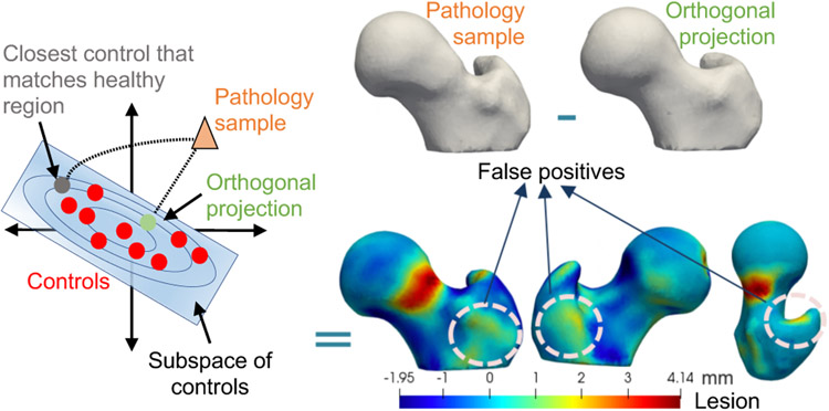
SSM can provide an objective characterization of a patient’s lesion extent by relating a patient-specific anatomy to the population-level shape statistics of controls. In particular, given a shape model trained on control subjects, a pathologic sample can be represented in the context of the controls population using its closed-form, orthogonal projection onto the PCA subspace of controls. The lesion can then be detected by quantifying the deviation of the pathologic shape from the shape reconstructed based on the model of controls. However, such deviation would result in false positives and fail to determine the accurate representation of the given pathology with respect to the controls’ model, primarily because the lesion is a localized abnormal shape change that is not explained by the controls’ statistics. If detected or known in advance, the lesion could be discarded, allowing only the healthy parts of the shape to predict the closest control shape to the given pathologic sample, similar to (Albrecht et al., 2013). In lesion screening, lesions are not known a priori, and hence representing a pathologic sample with respect to the controls’ statistics should down-weight the lesion in the projection of the pathologic shape to reduce false positives in the lesion identification process (Fig. 10).
Fig. 10.
Pathology sample projection onto controls’ subspace. Orthogonal projection of the pathology sample onto controls’ subspace falls to determine the accurate representation of the given pathology due to lesion being unsupported by the controls’ statistics. Hence, down-weighting the lesion in the projection of the pathology sample via an iterative optimization can help determine the closest control that matches the healthy region.
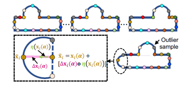
To reduce false positives, we formulate the projection onto the controls’ subspace as an optimization problem that simultaneously estimates the sample’s projection and identifies the anatomical regions not supported by the controls shape model. The optimization is formulated using a slack-variables-based approach. In particular, slack variables or surface offsets capture the pointwise differences in the surface normal direction between the pathology sample and the reconstruction of the pathology sample with respect to the controls statistics. Since we do not know in advance whether a sample is control or pathology, offsets should be minimal in the case of a control subject, and thereby the solution to this nonorthogonal projection should converge to that of the orthogonal projection. Furthermore, surface offsets should only be nonzero for those point correspondences that belong to the spatial support of the lesion. Hence, the nonorthogonal projection of a pathology sample to the closest control match is formulated as the solution of the following energy function that balances the trade-off between surface reconstruction based on a pre-trained shape model and a sparsity inducing regularization for the surface offsets.
| (1) |
where:
is a pathology sample represented as M–correspondence points for i ∈ {1, …, M}, and d = 3 for 3D shapes.
The controls PCA subspace is parameterized by Θ = {μ, U}, where is the mean shape and are the dominant K–eigenvectors, i.e., modes of variation, explaining 97% of the variability in the population.
is the orthogonal projection (i.e., shape parameters) of a pathology sample onto a controls PCA subspace.
denotes the reconstructed pathology correspondences from the controls PCA subspace, computed in closedform as x(α) = Uα + μ, with an orthogonal projection of shape parameters α.
represents the i–th reconstructed correspondence point. To avoid the clutter of notations, we removed the explicit dependency of the reconstructed correspondences on the pretrained shape model, i.e., xi(α) = xi(α∣Θ).
is the surface normal vectors for the correspondences on the pathology reconstruction and is the normal vector of the i–th correspondence xi(α).
is vector of surface offsets for the correspondence points on the pathology reconstruction. represents a vector of offsets with equal elements Δxi(α) for the i–th correspondence in the direction of surface normal η(xi(α)) on the shape x(α).
∘ denotes elementwise (i.e., Hadamard) product.
λ is the regularization parameter of the sparsity prior on the surface offsets to force zero offsets for regions/samples that are explained by the controls statistics.
The energy function in (1) is minimized using gradient-descent optimization. The derivation of the objective gradient and the algorithm for slack variables optimization are detailed in Appendix B. The gradients obtained are used to minimize the objective function in an iterative manner using an adaptive learning rate (see Algorithm 1 in Appendix B). The parameters that minimize the energy function in (1) are used to compute the closest control to the given pathology sample x(α), and the offsets Δx(α) indicate the extent of the lesion.
The offsets are used to validate the performance of the SSM tools in identifying the lesion. A qualitative assessment of shape models from SSM tools is performed as follows: (1) the group differences between the original controls, held-out samples, and the reconstructed controls with offsets are not expected to provide any significant differences because the shape model should explain controls variability; and (2) the group differences between the pathology and the reconstructed pathology samples with offsets are expected to inform differences localized to a particular region. The group differences are visualized, and the offset values are assessed across shape models.
The estimated offsets are also used in a pathology classification task (Fig. 6). A random train and test split is performed on the controls and pathology samples. The offsets of the training samples are fed to a multilayer perceptron classifier, with labels 0 and 1 indicating control and pathology, respectively. The accuracy of the classifier is then obtained by testing the model on the test, held-out samples, consisting of controls and pathology subjects. Multiple train-test splits are performed, and the average accuracy of the classifier is reported for each SSM tool.
5. Results
This section presents the evaluation and validation results of the considered SSM tools (Section 3.1) for a representative set of clinical applications (Section 3.2) that demonstrate common and important clinical utilities of shape modeling. The time and memory analysis for generating shape models using ShapeWorks and Deformetrica are detailed in Appendix C.
5.1. Experimental setup
Here, we cover datasets and training/testing splits for building shape models considered for the benchmark study.
5.1.1. Datasets
The segmented binary volumes of each of the following datasets were preprocessed as detailed in Section 4.
Left atrial appendage (LAA).
The population study was conducted on 130 LAA images that were retrospectively obtained from the AFib database at the University of Utah. The LAA dataset is representative of the AFib population (Navaravong et al., 2014). The MRI images were served with a single-handed segmentation by an expert. The ground-truth landmarks consisting of five points on the LAA ostium were manually annotated for each LAA sample using Corview (Marrek inc., Salt Lake City, UT), as shown in Fig. 2(f), and reviewed by a clinical expert.
Scapula.
CT scans and corresponding scapula segmentations of 31 cadaveric control scapulae and 54 scapulae of patients with shoulder instability were obtained from the coracoacromial morphology study in (Jacxsens et al., 2019). The results from the study provide support to conduct further research on all types of shoulder instability using CT scans. Furthermore, an explanation was provided in (Jacxsens et al., 2019) to justify and rule out any bias involved in the controls and pathology samples. The anatomical landmarks obtained for the scapulae participants under the coracoacromial morphology study were used here for the validation of the landmarks inference. The ground-truth landmarks were manually annotated for six curves, as shown in Fig. 3(b). A best-fit circle of the glenoid was used for the glenoid landmark annotation. The significance of such landmarks is as follows: Curve 1 landmarks represent the anatomy of acromion, curves 2 and 3 landmarks capture the coracoid process, curve 4 and 5 landmarks obtain the curvature of the concave articular surface of the glenoid, and curve 6 landmarks encode the anterior rim of the glenoid to address potential anterior defects. These landmarks are of interest to address both the glenoid and the coracoacromial anatomy to understand the pathoanatomy and pathomechanics of shoulder instability. The data as part of the coracoacromial morphology study (Jacxsens et al., 2019) were preprocessed as follows- The left scapulae shapes were mirrored to right scapulae shapes to ensure a consistent orientation of all the shapes in the cohort. Scapulae shapes were aligned to the glenoid-based coordinate system.
Humerus.
CT scans and humerus segmentations of 31 cadaveric control humeri and 54 humeri of patients with shoulder instability and a Hill-Sachs lesion were obtained as part of the study in (Jacxsens et al., 2019). The ground-truth landmarks were obtained for three anatomical curves, as shown in Fig. 3(c), which encode the morphological information of the humeral head. Information on the articular surface is encoded in curves 1 to 3 (Fig. 3(c)). The inference of these landmarks can help in surgical planning.
Femur.
The femurs data were collected through CT scans of 59 control and 37 FAI patients with cam-type lesions. These scans were obtained as part of the cortical bone thickness study (Atkins et al., 2017b). The demographics of all the patients were analyzed using the Wilcoxon rank sum test. The metrics between the sub-groups of male and female control and cam subjects were not signicantly different.
5.1.2. Train/test splits and shape modeling
We used importance sampling as detailed in section 4.1 to define random training/testing data splits for each dataset. For each random split, the training data were fed to each SSM tool to build the shape model. Since ShapeWorks and Deformetrica rely on a groupwise optimization approach, the point correspondences for each of the test samples were obtained by using the mean shape for initialization and fixing the correspondence of the training samples (i.e., the shape model). Due to its pairwise approach, the process of obtaining the correspondences for each test sample from SPHARM-PDM is the same as training. Specific details on the training/testing splits for each dataset are presented in the following paragraphs.
LAA.
Using the elbow method (Hardy, 1994), the number of clusters in the LAA dataset was identified as four, matching the LAA morphology classification reported in the literature (Wang et al., 2010). Seventy percent of the samples were selected using random sampling without replacement from each cluster to serve as training data. The remaining samples from each cluster were considered as testing data. Two such random train and test splits were sampled to perform the analysis.
Scapula.
Controls and pathology cohorts were used to generate two random splits. Split-1 had controls as training data and pathology samples as testing, whereas split-2 was constructed with pathology samples as training data and controls as testing data. The purpose of these splits is to assess the performance of SSM tools in inferring landmarks for both control and pathology subjects when trained using only the morphology of one of these groups. Testing samples of controls and pathology for split-1 and split-2, respectively, were randomly sampled without replacement using a 75%/25% train/test split to validate landmark inference on held-out samples from the same group considered to build the shape model of each split.
Humerus.
Two random splits, split-1 and split-2, were defined similarly to the scapula dataset.
Femur.
The data split for the femurs was random, and the split-1 and split-2 (similar to the scapula dataset) were used for evaluation. Split-1 alone was used for lesion screening.
5.2. Evaluation results
Evaluation of shape models is performed using quantitative and qualitative metrics detailed in Section 4.2. The compactness and specificity metrics are obtained using the training data. The generalization metric is computed as the ability of the shape model to represent held-out samples.
5.2.1. LAA shape models
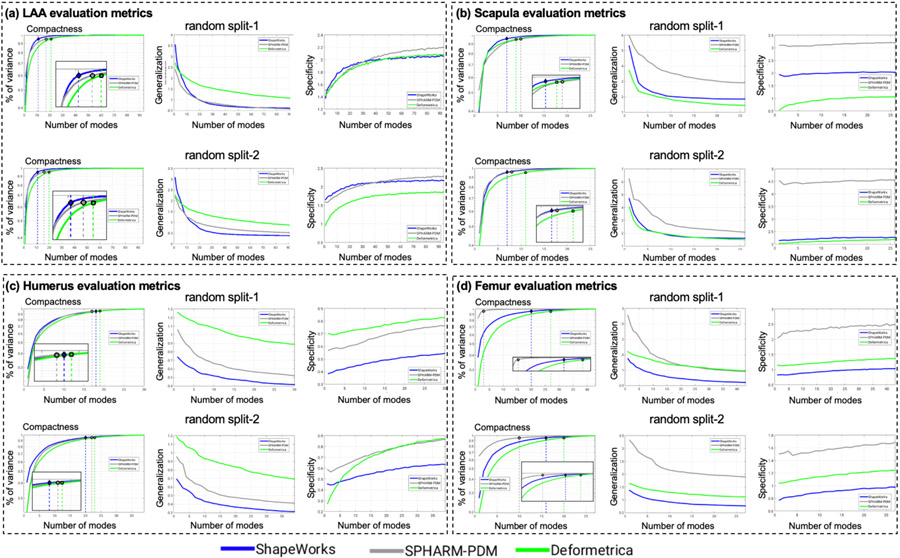
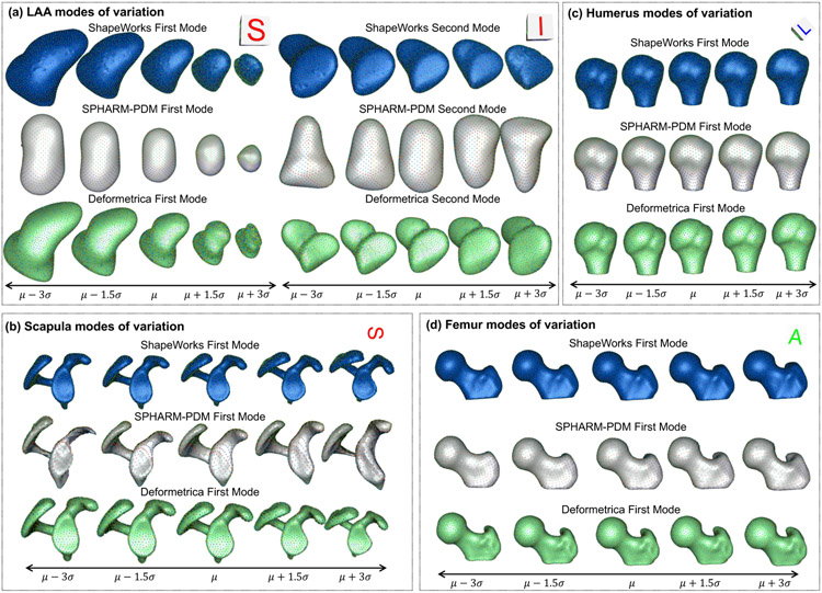
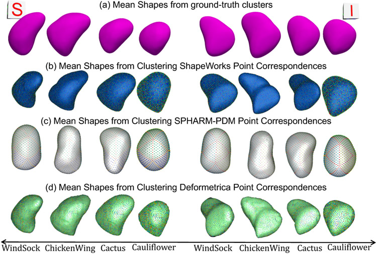
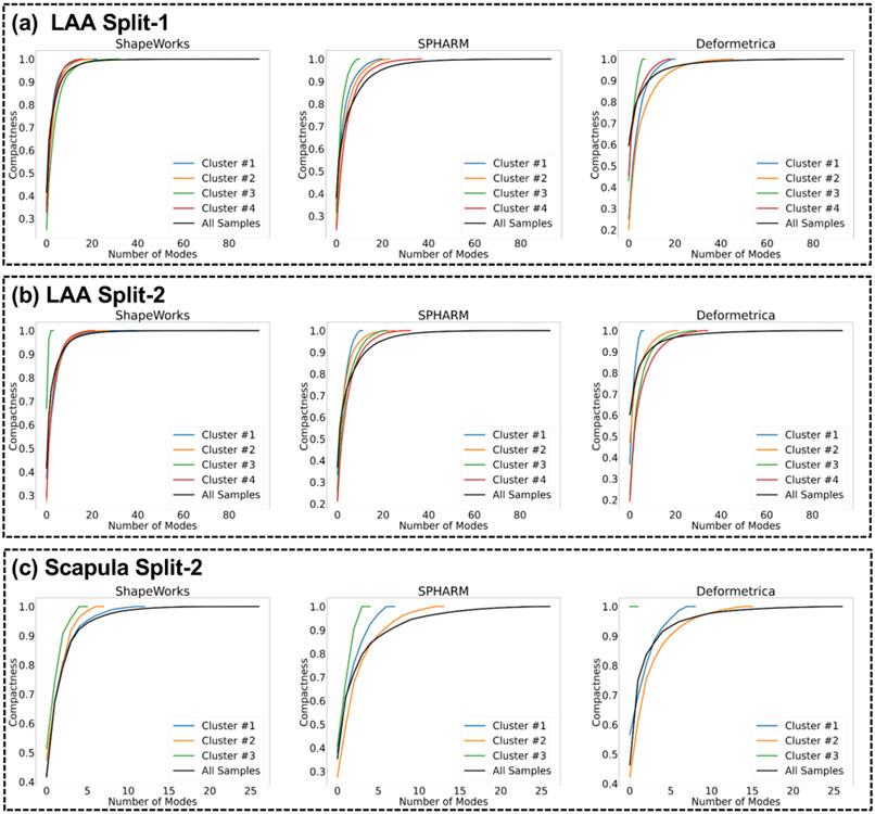
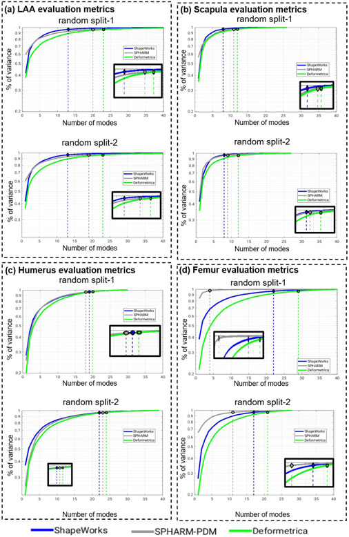
Fig. 12(a) shows the quantitative metrics (compactness, generalization, and specificity) of LAA shape models trained using the two random splits. ShapeWorks consistently produced a compact model compared to SPHARM-PDM and Deformetrica (first column). ShapeWorks generalization was comparable to SPHARM-PDM for split-1 with a better performance for split-2 and better than Deformetrica in estimating the shape representation of unseen samples (second column). Deformetrica outperformed ShapeWorks and SPHARM-PDM in the specificity measure for split-2 and with an increasing number of modes in split-1, ShapeWorks’ specificity became comparable to Deformetrica (third column). Fig. 13(a) demonstrates the first two dominant modes of variation from the entire dataset without any splits. ShapeWorks and Deformetrica models were able to discover clinically relevant modes of variation in the data, which are elongation of the appendage and ostia size. The SPHARM-PDM model could discover neither the representative shape nor the dominant modes of variation correctly. The clustering analysis was performed on all the samples without any training and testing splits. Four clusters were identified in the data using the elbow method. The ability of shape models to discover the natural clusters was assessed as follows: The signed distance transform (DT) images were clustered using K-means, and the mean shape from each cluster was obtained to serve as a baseline. The ground-truth cluster labels for all the input shapes were manually annotated and reviewed by a clinical expert. The point correspondences from each shape model were clustered, and the cluster centers discovered from each tool were qualitatively compared to the mean shapes of the ground-truth clusters. The results illustrated in Fig. 14 suggest that ShapeWorks and Deformetrica were able to discover the natural clusters in the data.
Fig. 12.
Compactness (higher is better), generalization (lower is better), and specificity (lower is better) computed for shape models of (a) LAA, (b) scapula, (c) humerus, and (d) femur random splits.
Fig. 13.
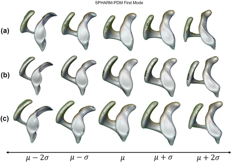
Shape modes of variation for (a) LAA, (b) scapula, (c) humerus, and (d) femur datasets. (a) Superior (S) and inferior (I) views are shown for LAA. (b) Superior (S) view is shown scapula. (c) Left (L) view is shown for humerus. (d) Anterior (A) view is show for femur.
Fig. 14.
Superior (S) and inferior (I) views of mean shapes from (a) ground-truth clusters, and k-means clustering of correspondences from (b) ShapeWorks (Cates et al., 2017a), (c) SPHARM-PDM (Styner et al., 2006), and (d) Deformetrica (Durrleman et al., 2014). Cluster centers from ShapeWorks and Deformetrica models closely align with the ground-truth cluster centers.
5.2.2. Scapula shape models
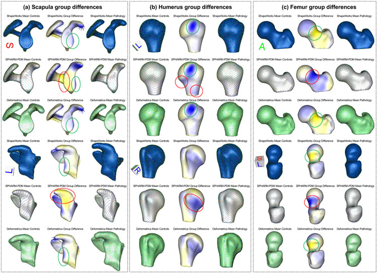
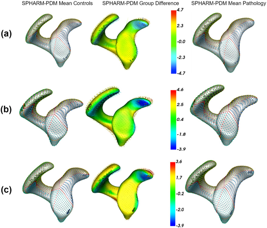
Fig. 12(b) shows the quantitative metrics of scapula shape models. ShapeWorks consistently produced a compact model compared to SPHARM-PDM and Deformetrica for the two random splits. The generalization of Deformetrica and ShapeWorks was comparable in modeling unseen samples, specifically with an increased number of modes, with a slightly better specificity in favor of Deformetrica for split-2 (second column). Deformetrica specificity was better than that of ShapeWorks and SPHARM-PDM in split-1. The Deformetrica and ShapeWorks specificity measure were comparable in split-2. However, Fig. 12(b) shows that SPHARM-PDM could not generalize well, and the samples generated by the shape model were not representative of the shape population in both splits. This performance is due to the complex morphology of the scapula compared to LAA. Fig. 13(b) shows the dominant modes of variation in the entire dataset for controls and pathology. ShapeWorks and Deformetrica were able to discover the clinically relevant mode of variation, which is the variation of the glenoid size due to an anterior glenoid defect in the pathology subjects in the population. However, SPHARM-PDM could neither produce a representative shape of the population nor encode a clinically relevant mode of variation. Furthermore, ShapeWorks and Deformetrica models were able to capture the clinically relevant group differences between the controls and pathology population (see Fig. 15(a)).
Fig. 15.
Mean controls, mean pathology, and group difference for (a) scapula, (b) humerus, and (c) femur anatomies. (a) Superior (S) and left (L) views are shown for scapula. (b) Left (L) and right (R) views are shown for humerus. (c) Anterior (A) and superior-left (S-L) views are shown for femur.
5.2.3. Humerus shape models
Fig. 12(c) shows the quantitative metrics of humerus shape models trained using the two random splits. SPHARM-PDM produced a compact model in split-1, and ShapeWorks produced a compact model in split-2. Nonetheless, the three SSM tools similarly struggle to find a compact representation for the humerus shape compared to the other anatomies under study. One might think that the humerus variability is nonlinear or multimodal, and hence computing compactness using PCA could result in a noncompact model. However, as we show in Appendix D, the three tools resulted in multivariate Gaussian distributions for the humerus training splits. One possible explanation is that the humerus anatomy has subtle localized shape variations that none of the SSM tools considered in this study were able to capture in a lower number of modes. Shapeworks outperformed both Deformetrica and SPHARM-PDM in generalizing well on held-out shapes and generating plausible and realistic shapes. The dominant modes of variation in the entire dataset were analyzed from the entire dataset consisting of controls and pathology. The first dominant mode of variation, which is the characterization Hill-Sachs lesion, as illustrated in Fig. 13(c), was identified correctly by all the models. Moreover, all the models were able to capture the clinically relevant group differences between the controls and pathology populations (see Fig. 15(b)). Nonetheless, models from SPHARM-PDM encoded differences that are not aligned with the underlying morphological characteristics of the Hill-Sachs lesion.
5.2.4. Femur shape models
Fig. 12(d) shows the quantitative metrics of femur shape models trained using the two random splits. SPHARM-PDM consistently produced a compact model compared to ShapeWorks and Deformetrica for the two random splits. The generalization of ShapeWorks was better than that of Deformetrica and SPHARM-PDM in modeling unseen samples. The specificity of ShapeWorks was better than that of Deformetrica and SPHARM in both splits. However, Fig. 12(d) shows that SPHARM-PDM could not generalize well, and the samples generated by the shape model were not representative of the shape population in both splits. The dominant modes of variation in the femur data were analyzed from the entire dataset consisting of controls and pathology. ShapeWorks and Deformetrica were able to discover the clinically relevant mode of variation, which is the extra bone growth in the femoral head (see Fig. 13(c)). However, SPHARM-PDM could not encode the clinically relevant mode of variation. ShapeWorks and Deformetrica models were also able to capture the clinically relevant group differences between the controls and pathology population (see Fig. 15(c)).
5.3. Validation results
The validation is conducted by comparing the ground-truth information with the predictions of the SSM tools.
5.3.1. Anatomical measurements inference – LAA
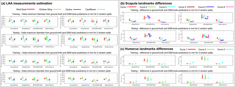
SSM tools were validated based on the accuracy of the LAA ostia measurement predictions. The ground-truth measurements were obtained, as shown in Fig. 2, where the landmarks on the LAA ostium were used to compute the ground-truth measurements of the LAA maximum and minimum diameters by fitting an ellipse to each LAA ostium. Fig. 16(a) shows the ground-truth measurements and SSM tool predictions for the LAA ostia maximum and minimum diameters for the training and testing samples. ShapeWorks and Deformetrica models predictions were closely aligned to the ground-truth compared to predictions from SPHARM-PDM models. LAA closure implant devices are available in increments of 2-4 mm (Akinapelli et al., 2015). Identifying a difference of 2 mm is clinically relevant for LAA closure implant design and selection. From Fig. 16(a), ShapeWorks and Deformetrica models predictions are mostly clinically relevant compared to predictions from SPHARM-PDM models.
Fig. 16.
Validation results of the (a) LAA ostia maximum and minimum diameter measurements, (b) scapula landmark differences, and (c) humerus landmark differences, from ground-truth and predictions of SSM tools in mm for the two random splits.
Statistical tests showed the equivalence of the predicted and ground measurements, based on Euclidean distances, for ShapeWorks and Deformetrica in split-1 for the maximum diameter (p = 0.569 and 0.210, respectively), and Deformetrica in split-2 (p = 0.436). When combining the splits with clusters, we found the equivalence for ShapeWorks, SPHARM-PDM, and Deformetrica (maximum diameter) for split-1-cluster-1, split-2-cluster-1, and split-2-cluster-2. In addition, when using Deformetrica, we found the equivalence (for maximum diameter) in all splits and cluster combinations except for split-1-cluster-4 (p = 0.037).
5.3.2. Anatomical landmarks estimation – scapula
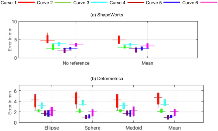
Fig. 16(b) shows the Euclidean distance between the ground-truth landmarks and landmarks inference from each SSM tool (average of the cumulative distances for the points/landmarks on each curve) for the six anatomical curves of scapula. We found smaller errors in the case of curves 4, 5, and 6 in the two random splits. The performance of the Deformetrica and ShapeWorks models is comparable and better than that of the SPHARM-PDM model. The measurement of the glenoid radius can be computed from the landmarks of curve 4. The glenoid radius was obtained from the ground-truth landmarks and inferred landmarks of the SSM tools.
In split-1, statistical tests showed the equivalence of the predicted and ground-truth measurements, based on the distances in Euclidean space, for the glenoid radius in ShapeWorks (p = 0.07 for no template for initialization and 0.09 for the mean template for initialization), for the distance between the apex of the coracoid process and anterolateral corner (ALC) of the acromion as well as the distance between apex of the coracoid process and the posterolateral comer (PLC) of the acromion in Deformetrica (p = 0.112 and 0.209, respectively, for the raw measurements; p = 0.416 and 0.140, respectively, for the ellipse atlas; p = 0.355 and 0.168, respectively, for the sphere atlas; p = 0.149 and 0.285 for the medoid atlas).
5.3.3. Anatomical landmarks estimation – humerus
The landmarks inference of Deformetrica and ShapeWorks was better than that of SPHARM-PDM, resulting in lower errors (see Fig. 16(c)). Curve 2 had lower errors compared to curves 1 and 3 in both test data predictions. The measurement humerus radius can be computed from the landmarks of curve 2. The humerus radius was obtained from the ground-truth landmarks and the inferred landmarks of the SSM tools. Statistical tests showed the equivalence of the predicted and ground truth measurements, based on Euclidean distances, for Deformetrica in split-1 for the humerus head radius (p = 0.09).
At present, orthopaedic companies size their shoulder implants in increments of 2-5 mm. Furthermore, shoulder instability has been observed with shape differences in the range of 2-5 mm (Jacxsens et al., 2019). Therefore, we believe that identifying a difference of 2 mm is clinically-relevant. From Fig. 16 (b) and (c), ShapeWorks and Deformetrica models predictions are mostly clinically relevant compared to predictions from SPHARM-PDM models, since they can predict shoulder joint measurements to the level of manufactured implants intended to replace them.
5.3.4. Lesion screening – femur and humerus
SSM tools were validated based on the lesion identification and the accuracy of the classification of the pathology. The lesion identification is qualitative because the ground-truth lesion is unavailable for the participants with pathology. The accuracy of classification of the pathology from shape models was obtained to quantify the performance.
Lesion identification:
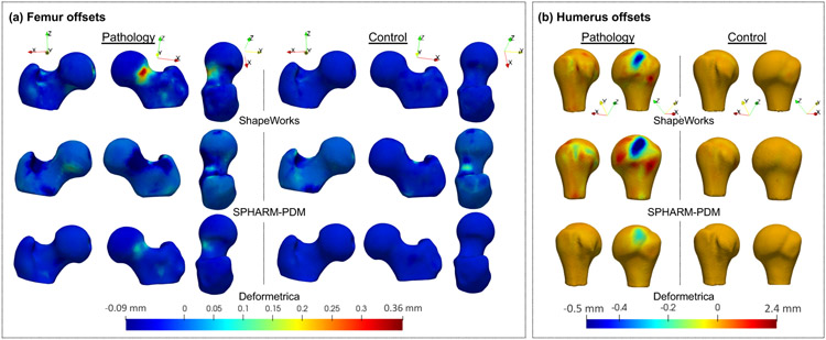
The slack variable optimization (Algorithm 1) resulted in the identification of the closest control to the pathology and captured the lesion in the slack variables or offsets in the normal direction of each correspondence point. The differences between the reconstruction and reconstruction with the offsets in the normal direction were visualized groupwise for all the control and pathology samples (see Fig. 17). The offsets for the controls did not signify a lesion, whereas the offsets for the pathology signified a lesion. For femurs, the lesion was correctly identified in the case pathological group differences by ShapeWorks and Deformetrica models (see Fig. 17(a)). For humeri, the lesion was correctly identified in the case of pathological group differences by all the models (see Fig. 17(b)). The SPHARM-PDM model captured false positives in the pathology differences compared to ShapeWorks and Deformetrica models (see Fig. 17(b)).
Fig. 17.
The group differences between the reconstructed samples and reconstructed samples with offsets. (a) Femur group differences for pathology (left) and controls (right). (b) Humerus group differences for pathology (left) and controls (right).
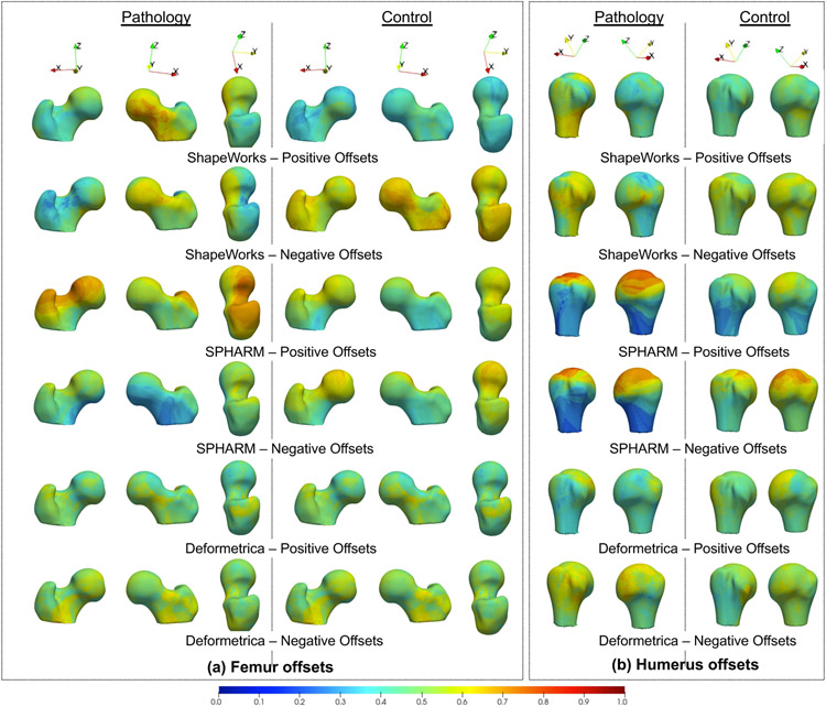
The lesion screening task must identify the spatial distribution of the estimated offsets on the anatomy’s surface. Here, we visualize the spatial trends of the estimated offsets using the held-out, unseen pathology and controls samples. Events of interest are positive offsets that reflect bone protrusions for femurs and negative offsets that reflect bone recession for humerus. We calculate the probability of a positive offset and a negative offset at each correspondence point for all the pathology and control held-out samples. The occurrence probabilities are calculated by counting the positive and negative offsets at a correspondence point and then dividing this count by the number of samples in the testing cohort (pathology or control). Both these probability values are then interpolated onto the mean mesh obtained from the shape model using the training data (i.e., controls seen). The results are presented in Fig. 18.
Fig. 18.
Positive and negative offset occurrence probability visualized on the mean training mesh for humerus and femur unseen pathology and controls
The positive and negative offset probabilities visualized for unseen femur and humerus controls in Fig. 18(a) (second column) and Fig. 18(b) (second column), respectively, mostly vary around 0.3 to 0.6 for ShapeWorks and Deformetrica in regions that are not spatially lesion-specific, indicating no prominent lesions detected across held-out control samples. SPHARM-PDM, on the other hand, shows higher probability values (around 0.8) for humerus controls, indicating increased false positives. Fig. 18(a) (first column) shows the offset probabilities for held-out femurs pathology, where ShapeWorks and SPHARM-PDM have higher positive offset probabilities as compared to Deformetrica. In contrast to Deformatrica, ShapeWorks results in positive offset probabilities that are better localized around the head-neck junction, which is the location for the cam-FAI protrusion. SPHARM-PDM, on the other hand, results in more positive than negative offsets. Nevertheless, the spatial distribution of positive offsets is distant from the cam-FAI lesion, resulting in higher false positives. Fig. 18(b) (first column) shows the offset probabilities for held-out humerus pathology, where ShapeWorks results in more spatially localized negative offsets compared to Deformetrica. SPHARM-PDM produces higher positive and negative offsets that are spatially less specific to the Hill-Sachs recession lesion.
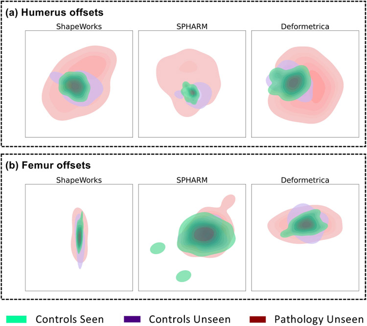
To analyze the high-dimensional distribution of the estimated offsets, we use t-Distributed Stochastic Neighbor Embedding (t-SNE) (Van der Maaten and Hinton, 2008) for dimensionality reduction. For each SSM tool, the offsets data, which is a scalar per correspondence point, from all three groups —pathology unseen, controls unseen, and controls seen— are pooled into a single data matrix. We then applied the t-SNE algorithm to map all the offsets to a 2D space to visualize the distributional differences between offsets estimated for pathology samples versus those estimated for controls. The 2D embedding obtained from t-SNE is then passed to a bivariate kernel density estimator, which determines the probability density of 2D embedding for the 3 groups. The visualizations of the embedding are shown in Fig. 19. The offsets for humerus across all tools show distinct clusters (Fig. 19(a)), indicating that the pathology and control offsets are discernible. This distinction is reflected in the classification results seen in Table 1(b), where the MLP classifier can better discriminate between the controls and pathology groups. The offsets for femurs do not show highly distinct clusters (Fig. 19(b)). SPHARM-PDM, in particular, shows overlapping densities for controls and pathology, which can be verified by the poor classification performance of SPHARM-PDM in Table 1(a) compared to ShapeWorks and Deformetrica.
Fig. 19.
Kernel density map of t-SNE clusters of all samples for (a) humerus offsets (b) femur offsets.
Table 1.
Pathology classification training performance from SSM tools
| (a) Femur pathology classification | ||||||
|---|---|---|---|---|---|---|
| Training performance | Testing performance | |||||
| Metrics ╲ SSM Tools | ShapeWorks | SPHARM-PDM | Deformetrica | ShapeWorks | SPHARM-PDM | Deformetrica |
| Accuracy (μ ± σ)% | 97.851 ± 0.025 | 77.851 ± 0.088 | 93.465 ± 0.03 | 83.167 ± 0.078 | 55.833 ± 0.085 | 83.833 ± 0.083 |
| FI Score (μ ± σ)% | 96.977 ± 0.033 | 60.681 ± 0.198 | 90.634 ± 0.043 | 81.125 ± 0.108 | 39.455 ± 0.203 | 80.89 ± 0.128 |
| AUC (μ ± σ) | 0.697 ± 0.109 | 0.378 ± 0.145 | 0.595 ± 0.278 | 0.613 ± 0.166 | 0.52 ± 0.298 | 0.57 ± 0.135 |
| (b) Humerus pathology classification | ||||||
| Training performance | Testing performance | |||||
| Metrics ╲ SSM Tools | ShapeWorks | SPHARM-PDM | Deformetrica | ShapeWorks | SPHARM-PDM | Deformetrica |
| Accuracy (μ ± σ)% | 98.73 ± 0.012 | 97.143 ± 0.019 | 93.651 ± 0.119 | 96 ± 0.033 | 95.333 ± 0.027 | 90.667 ± 0.122 |
| FI Score (μ ± σ)% | 98.912 ± 0.01 | 97.619 ± 0.015 | 92.824 ± 0.137 | 96.157 ± 0.029 | 95.108 ± 0.031 | 87.46 ± 0.188 |
| AUC (μ ± σ) | 0.829 ± 0.134 | 0.853 ± 0.07 | 0.796 ± 0.262 | 0.88 ± 0.102 | 0.822 ± 0.13 | 0.762 ± 0.349 |
Pathology classification:
The offsets obtained from the optimization process were fed to a multilayer perceptron with labels 0 and 1 indicating control and pathology, respectively. The dataset was randomly split into training and testing sets. The best set of hyperparameters (activation, hidden layers, number of units in each hidden layer, regularization, and solver) was found using three-fold cross validation on the training data of each SSM tool independently. The model was then trained using the training data with the best set of hyperparameters and used for the classification of pathology on the test data. The random train-test split, hyperparameter tuning, and testing were performed for several iterations to obtain the average predictions from the trained models. Classification performance metrics were obtained from the trained models on the training and testing data (see Table 1). In the case of the femur, the performance of ShapeWorks and Deformetrica trained models was comparable (see Table 1(a)). The standard deviation of metrics was low for ShapeWorks, indicating the minimal deviation of the results for different train-test splits. SPHARM-PDM results were inferior in the classification of pathology. In the case of the humerus, the performance of ShapeWorks trained model was better than that of Deformetrica and SPHARM-PDM (see Table 1(b)). SPHARM-PDM model performance was comparable to that of ShapeWorks. The standard deviation of metrics was relatively higher for Deformetrica-trained models. The larger generalization error of all the SSM tools for the femur data compared to the humerus data. This performance complies with the better clusterability of the offsets’ tSNE embedding for the humerus data compared to the femur data (see Fig. 19. This performance difference may be attributed to the differences in balance of classes in the two datasets. In particular, femurs had 37 pathology and 59 control samples, whereas humerus had 52 pathology and 41 control samples. The humerus data is more balanced than the femur. The imbalance in the dataset could be one possible reason for the inferior performance statistics.
6. Discussion
ShapeWorks produced shape models with consistent quantitative and qualitative performances in most of the experiments detailed in the results section. This consistency can be attributed to the underlying groupwise correspondence-based approach. For evaluation metrics, ShapeWorks resulted in compact models of the LAA, scapula, and humerus anatomies (see Fig. 12). ShapeWorks models generalized well for the LAA, scapula, humerus, and femur anatomies, and consistently generated plausible shapes of the scapula, humerus, and femur anatomies. ShapeWorks models were able to discover clinically relevant modes of variation, including the group differences for all the studied anatomies, and the natural clusters in LAA (see Fig. 14) and its validation outcomes were closely aligned to the ground-truth.
Deformetrica models were comparable to those of ShapeWorks in a few experiments due to the underlying groupwise deformation-based approach. However, Deformetrica results were not consistent throughout the experiments because of the impact of the input atlas that needs to serve as an initialization. A qualitative assessment of the performance of Deformetrica models with different atlases was performed on an ensemble of 3D shapes of boxes with a moving bump. The first mode of variation from the Deformetrica models with different input atlases (mean, medoid, random input, ellipsoid, and sphere) resulted in large variability in the first mode of variation (see Fig. 20). The ellipsoid and sphere atlases were scaled to match the input shapes. The variability displayed in the discovery of the moving bump informs the inconsistency in the Deformetrica models. When the medoid was provided as an input atlas to Deformetrica, the moving bump in the first mode of variation was closely aligned to the ground-truth. The modes of variation for the mean and ellipsoid input atlases were similar. A quantitative assessment of the performance of Deformetrica models with different atlases was performed on scapula landmarks inference task. The algorithm could not produce a good shape model when the input atlas was provided as an ellipse and sphere. Hence, the sphere and ellipsoid were deformed onto some subject as a preprocessing step. The deformed sphere and ellipsoid at an intermediate step of the deformation flow were then used as modified initial atlases. The Euclidean distance between the ground-truth and predicted landmarks from the Deformetrica models with different input atlases (ellipsoid, sphere, medoid, and mean) resulted in different levels of errors (see Fig. 21 (b)). ShapeWorks does not need an input atlas to generate point correspondences. To analyze the performance of ShapeWorks with an input atlas, the point correspondences of the training data were initialized to the mean training shape. The Euclidean distance between the ground-truth and predicted landmarks with no reference and mean shape initialization was compared (see Fig. 21 (a).).
Fig. 20.
Box bump mode of variation of Deformetrica with the input atlas as (a) the medoid, (b) the mean, (c) a random shape, (d) an ellipsoid, and (e) a sphere, producing different shape statistics.
Fig. 21.
Quantitative assessment (scapula landmarks inference task) of SSM tools with different input atlases on the unseen samples. (a) ShapeWorks with no reference and input initialization as a mean shape, (b) Deformetrica with input atlases as ellipse, sphere, medoid, and mean shapes.
SPHARM-PDM models mostly displayed inferior results compared to those of Deformetrica and ShapeWorks in the evaluation and validation experiments. This inferior performance can be attributed to the pairwise correspondence-based approach that does observe the entire cohort, where the correspondences from SPHARM-PDM are generated by mapping every input shape to a unit sphere. This spherical mapping can result in ambiguity in the mapping of the axes demonstrated in the LAA modes of variation (see Fig. 13(a)). In the case of evaluation metrics, SPHARM-PDM could not produce compact models of the anatomies LAA, scapula, and humerus (see Fig. 12). SPHARM-PDM models could not generalize adequately for the scapula, humerus, and femur anatomies, and could not generate plausible shapes for all the anatomies. The SPHARM-PDM models could not consistently discover clinically relevant modes of variation, including the group differences, and were unable to discover natural clusters in LAA (see Fig. 14). SPHARM-PDM validation outcomes were rarely aligned to the ground-truth.
In summary, the SSM tools produced different levels of consistency in the evaluation and validation process, which indicates the need for such an assessment in real-world clinical applications. Based on the overall results from all the experiments, we can infer that the groupwise correspondence technique can potentially learn the population-level variability compared to the pairwise correspondence method.
7. Conclusion and future work
The main contribution of this work is a systematic evaluation and validation of open-source statistical shape modeling (SSM) tools in the context of clinical applications, an area in which there has been little work (Gollmer et al., 2014).
7.1. Research contributions
In this paper, we have presented an evaluation and clinically driven validation framework to assess the performance of shape models from different open-source SSM tools. Quantifying the performance of shape models is a challenging task due to the lack of ground-truth correspondences. This problem has been addressed by considering qualitative and quantitative metrics to determine the utility of shape models in clinical applications. The evaluation of shape models is performed using quantitative metrics such as compactness, generalization, specificity (Davies et al., 2002), and qualitative metrics, including modes of variation and clustering analysis. The validation of shape models is performed based on the differences between ground-truth and SSM tool predictions of anatomical measurements and class. The evaluation and validation framework is tested on representative real-world clinical applications such as implant design and selection, motion tracking, surgical planning, bone resection, and bone grafting. Different tools produced different levels of consistencies, which highlights the importance of such an assessment. ShapeWorks (Cates et al., 2017a) and Deformetrica (Durrleman et al., 2014) models displayed better results in the clinical applications compared to SPHARM-PDM (Styner et al., 2006) models due to the underlying groupwise approach for establishing shape correspondences. Deformetrica models displayed inconsistencies in results due to the bias introduced by the input atlas used for initialization. SPHARM-PDM models were inferior in performance due to the underlying pairwise correspondence approach. The evaluation indicated that SPHARM-PDM models mostly were unable to produce compact models, generalize well to unseen shapes, and generate realistic shapes that retain the shape characteristics of the population under study. SPHARM-PDM models could not discover clinically relevant modes of variation and could not identify natural clusters in a morphology such as LAA, due to ambiguity in the mapping of the axes. The validation demonstrated that ShapeWorks and Deformetrica models were comparable in performance and outperformed SPHARM-PDM models.
7.2. Scientific impact
This research provides a direction to systematically assess different SSM tools available for clinical applications. The framework assists in selecting and deploying the right SSM tool to address a clinical need. The assessment of SSM tools can motivate further research and enhancement of the underlying optimization techniques involved in shape-modeling tools. Benchmarking the performance of shape models could motivate the development of a new class of shape-modeling tools and techniques, which could take the performance of SSM in real-world applications to another level. This study may also drive the development of a new set of tools to automate the end-to-end evaluation and validation of SSM tools, when given training and test data. The evaluation and validation framework proposed in this paper could easily be extended to other clinical situations or other classes of applications of SSM.
7.3. Limitations and future work
This research is confined to three open-source, widely used, state-of-the-art SSM tools applicable for general anatomies. However, the framework can be adapted to other SSM tools that work on general purpose anatomies or SSM tools that are tailored to specific anatomies. The performance results of the SSM tools discussed in this paper cannot be baselined for all the clinical applications or other clinical scenarios. The results from SSM tools can vary based on the various steps followed in the shape-modeling process, such as training data collection, data preprocessing, and parameter tuning for the shape models. The hyperparameter tuning process was performed for ShapeWorks and Deformetrica but not SPHARM-PDM due to its pairwise approach. High-quality training data can help improve the shape-modeling process. In the future, this study can be extended to other publicly available tools and clinical applications to benchmark SSM tools in different scenarios and to provide a blueprint for the development of computational methods, tools, and techniques for shape modeling.
Acknowledgements
This work was supported by Coherex Medical and the National Institutes of Health under grant numbers NIBIB-U24EB029011, NIAMS-R01AR076120, NHLBI-R01HL135568, NIBIB-R01EB016701, and NIGMS-P41GM103545. The content is solely the responsibility of the authors and does not necessarily represent the official views of the National Institutes of Health. This work was also partly funded by the European Research Council under grant number 678304, European Unions Horizon 2020 research and innovation program under grant number 666992, and program Investissements d’avenir under grant number ANR-10-IAIHU-06. The authors would like to thank the Division of Cardiovascular Medicine (data were collected under Nassir Marrouche, MD, oversight and currently managed by Brent Wilson, MD, PhD) and the Orthopaedic Research Laboratory (ORL) at the University of Utah for providing the MRI/CT scans and the corresponding segmentations of the left atrium appendage, femur, humerus and scapula, with a special thanks to Evgueni Kholmovski for assisting in MRI image acquisition. Authors acknowledge Christine Pickett and Riddhish Bhalodia for proof-reading the manuscript. The authors would also like to thank the anonymous reviewers for the time and expertise they have invested in their constructive reviews.
Appendix
Appendix A. SSM tools: technical details
Appendix A.1. ShapeWorks
PSM formulation treats each surface as a collection of interacting dynamic particles with mutually repelling forces to optimally cover, and therefore describe, the surface geometry. The correspondences are freely moving particles, yet they are constrained to lie on the surface, and their positions can be directly optimized. This particle-based representation avoids many of the problems inherent in parametric representations such as the limitation to specific topologies, processing steps necessary to construct parameterizations, and bias toward model initialization using initial atlases.
PSM optimization can be summarized as follows: Consider an ensemble of N shapes , each with its own set of M particles (i.e., correspondences) , where ordering implies correspondence among shapes. A correspondence lives in a d–dimensional space, i.e., , with d = 2 and 3 for 2D and 3D shapes, respectively. For groupwise modeling, a rigid or similarity transformation Tn is estimated to transform the particles in the n–th shape local coordinate system to the common coordinate system such that . This representation involves two types of random variables (Fig. 1(a)): a shape space variable and a particle position variable that encodes the distribution of particles on the n–th shape (configuration space). Correspondences are optimized by minimizing a combined shape correspondence and surface sampling objective function , where H is an entropy estimation assuming Gaussian shape distribution in the shape space and Euclidean particle-to-particle repulsion in the configuration space. This formulation favors a compact ensemble representation in shape space (first term) against a uniform distribution of particles on each surface for accurate shape representation (second term).
Appendix A.2. Deformetrica
The diffeomorphic multiobject template complex construction is performed using a Bayesian framework (Gori et al., 2017). The complex of a shape instance is modeled as a deformed template complex and a residual. The n–th shape complex is defined as Sn = ϕn(A) + ϵn, where ϕn(A) is the deformation on the template (A) specific to the n–th shape instance,, and ϵn is the residual. The variations in the shapes are modeled by these deformations, and each deformation is characterized by a set of parameters αn. The assumption here is that the parameters follow a Gaussian distribution, with a mean 0 and a covariance matrix Γα. The objective function is defined as estimating the template complex and covariance matrix by maximizing the joint posterior distribution of the shape complexes, i.e., . The maximization process is constrained by the requirement that the template complex should deform to match the shape complex, and the residual ϵn should be small.
Appendix A.3. SPHARM-PDM
SPHARM basis functions are defined with degree l and order k, , where θ ∈ [0; π], ϕ ∈ [0; 2π], and the associated Legendre polynomials. The surface of the n–th shape can be expressed using SPHARM basis functions by decomposing 3 coordinate functions that define the surface as xn(θ, ϕ) = (xn(θ, ϕ), yn(θ, ϕ), zn(θ, ϕ))T, and the surface would be of the form , where are 3D coefficient vectors due to the 3 coordinate functions. These coefficients are obtained using a least-squares method to fit the n–th shape surface. A correspondence point on the surface is given by a parameter vector (θm, ϕm), which represents the m–th location on the predefined sphere parameterization.
Appendix B. Slack variables-based optimization
| Algorithm 1 Nonorthogonal sample projection using slack- variables-based optimization | |
|---|---|
|
|
The energy function in (1) is minimized using gradient-descent optimization with an alternating coordinate descent on the parameters α and Δx(α). The L2 norm on the difference between the pathology sample and the reconstructed sample is minimized by encoding the differences attributed to the lesion variations not supported by the shape model in the surface/point offsets. The L1 regularization is used to induce sparsity on the offsets by allowing the differences to be captured only for the points not supported by the PCA subspace of the control (Fig. 11). The partial derivatives with respect to α are as follows:
| (B.1) |
Fig. 11.
Illustration of nonorthogonal sample projection optimization using slack variables (surface offsets). Box bump data with an outlier having a bump on the side. The offsets are captured for the points on the side bump alone as the side bump is not present in the rest of the samples.
Using the closed-form orthogonal reconstruction of a pathology from the PCA subspace, the vector representation of the gradient computation is given as
| (B.2) |
where . In an alternating coordinate descent, surface offsets Δx(α) are assumed to be fixed (i.e., lagging) with respect to α. The derivative computations of surface normals η with respect to α are approximated using finite differences across iteration (t) and (t − 1), with a vector representation written as
| (B.3) |
Gradients from (B.3) result in a matrix , which is summed with the gradients from (B.2) and multiplied with the vectorized form of , which is , resulting in a gradient.
For a given correspondence point offset, the partial derivatives of Δxi(α) are computed as follows:
| (B.4) |
where
| (B.5) |
L1 norm is a nondifferentiable penalty. Here, we use a smooth approximation to the L1 penalty consisting of the sum of the integral of 2 sigmoid functions defined by Schmidt (Schmidt et al., 2007), where β = 106 results in the approximation that is within a small-enough tolerance for the results produced by constrained optimization methods.
| (B.6) |
Hence, the gradient of the L1 norm approximation can be written as
| (B.7) |
Equations (B.5) and (B.7) are for a given point correspondence. Considering all the M points on a pathology reconstruction, (B.5) results in gradients in when converted from a flattened vector in to 3D points. Equation B.7 obtains gradients in . The gradient from (B.5) is multiplied by the converted to 3D points in and summed up across the resulting gradients of the dimensions in . These results are summed with the gradients from (B.5) to get the final gradients in .
Appendix C. Computational analysis
As discussed in section 4.3.1, ShapeWorks and Deformetrica use groupwise correspondence approaches to learn a population-specific atlas (i.e., mean shape) from the training samples. The mean shape can then be used to estimate the surface correspondences for the testing samples. This process can be performed in parallel for each testing sample. On the other hand, SPHARM-PDM uses a pairwise correspondence and allows correspondence estimation in parallel for individual data samples, including both training and testing samples. As SPHARM-PDM allows parallel computation on an as-needed basis, we compare only the computational performance involved in the training process for ShapeWorks v6.0 and Deformetrica v4.3.0.
For the computational performance analysis, we compare the time and memory utilization of ShapeWorks and Deformetrica for the training process of the 4 datasets and their corresponding two train/test data splits. All the experiments were run serially on a dedicated machine with the following configuration: OpenSUSE Leap 15.2, 16 CPU Intel(R) Core(TM) i7-9800X CPU @ 3.80GHz,x86_64 architecture. The results are consolidated in Table Appendix C.1.
ShapeWorks requires less time as compared to Deformetrica for the training process of the same dataset size. Whereas, Deformetrica, on average, has lower memory utilization. Nevertheless, ShapeWorks scales well for large datasets,which this can be observed by comparing the memory utilization for the LAA dataset.
Appendix D. Normality assumption of the shape models
PCA assumes linear correlations, and hence a multivariate Gaussian shape model. Gaussianity could be a simplifying assumption when using PCA to compute a model’s compactness. Specifically, a very compact non-Gaussian model (e.g., nonlinear, multimodal) might appear less compact through the lens of PCA. Here, we report the results of statistical normality tests on all the shape models to justify the use of PCA for computing the compactness metric in 4.2.
The null hypothesis is the data follows multivariate normal (i.e., Gaussian) distribution. A necessary but not sufficient condition for a multivariate distribution to be normal is that all marginals have to be univariate normal (Small, 1980). Two important properties of a dM–dimensional multivariate random variable Z with a multivariate normal distribution are:
All dimension subsets of the vector Z have a normal distribution.
Linear combinations of Z are normally distributed.
Considering the properties mentioned above and the computational efficiency of performing univariate tests, we test the normality hypothesis by conducting a Shapiro-Wilk (Shapiro and Wilk, 1965) normality test for each dimension in a shape model, with a total of dM–univariate normality tests for each shape model. For each dimension, if the p-value is > 0.05, we can accept the null hypothesis, and hence this dimension comes from a univariate normal distribution. For a shape model, if more than half dimensions of a model are univariate normals, then we deem the shape model as a multivariate normal distribution.
Table Appendix C.1.
Computational performance benchmarking results for the training process of ShapeWorks v6.0 and Deformetrica v4.3.0. Lower memory/time is bolded.
| Dataset ╲ SSM Tools | Time (hours) | Memory (gigabytes, GB) | Training Sample Size | ||
|---|---|---|---|---|---|
| ShapeWorks | Deformetrica | ShapeWorks | Deformetrica | ||
| Humerus Split-1 | 0.62 | 3.80 | 1.80 | 0.78 | 30 |
| Humerus Split-2 | 0.85 | 4.77 | 1.80 | 0.89 | 39 |
| Scapula Split-1 | 0.92 | 2.22 | 1.39 | 0.81 | 26 |
| Scapula Split-2 | 0.92 | 4.95 | 1.80 | 0.83 | 27 |
| Femur Split-1 | 0.92 | 1.67 | 3.96 | 0.81 | 44 |
| Femur Split-2 | 0.63 | 0.88 | 2.68 | 0.90 | 44 |
| LAA Split-1 | 2.60 | 15.36 | 1.34 | 1.90 | 94 |
| LAA Split-2 | 2.55 | 10.37 | 1.36 | 1.90 | 94 |
Normality tests are conducted on the training splits for each dataset since the compactness metric is associated with the training data. Results are summarized in Table Appendix D.1. The models generated by ShapeWorks are consistently multivariate normals for all anatomies except for LAA, which complies with existing literature on the natural clustering of LAA morphology (see section 3.2.1). Hence, a strong shape model should reflect such a multimodal shape distribution, which can be modeled using a mixture of Gaussians. Deformetrica, on the other hand, does not consistently produce multivariate normal models for datasets that have no known morphological clusters. Furthermore, Deformetrica does not reflect the multimodal structure of LAA shapes for one of the training splits. SPHARM-PDM is fairly consistent in producing multivariate normal shape models. However, it does not capture the clusterings of LAA shapes for one of the training splits.
To test the multimodality assumption of complex anatomies, we perform k-means clustering and use the elbow method (Hardy, 1994) to identify the optimum number of clusters for each shape model. Each cluster is tested for normality following the method explained above. All clusters from all shape models produced by the 3 SSM tools were found to follow multivariate normal distributions. In the case of Scapula split-2, where Deformetrica failed the normality test, we performed a similar clustering analysis. All clusters were labeled as multivariate normals except one cluster, which did not have enough samples for performing the normality test (Deformetrica cluster-2). In Fig. Appendix D.1, we report compactness curves for each cluster versus all training data for the LAA splits and the Scapula split-2. We expect that clusters of a multimodal distribution are either more compact or on par with the compactness of the entire training cohort which is is true for ShapeWorks and SPHARM. However, Deformatica shows some discrepancies, especially with lower number of modes. Deformetrica’s shape model of the LAA split-2 is not a multivariate normal distribution, yet 2 clusters out of 4 are less compact at lower modes compared to all samples from the training cohort. Similar to LAA split-2, the LAA split-1 shape model was found to be a multivariate normal distribution. For Scapula split-2, 2 of 3 clusters are less compact, for a shape model that passed the normality test.
Fig. Appendix D.1.
Cluster-level compactness of LAA splits and Scapula split-2.
Appendix E. Kernel principal component analysis
PCA attempts to find a linear subspace of lower dimensionality than the original data space. The axes of this subspace align with data directions of maximum variability. Standard PCA allows only linear dimensionality reduction. However, if the data manifold is nonlinear or multimodal, it cannot be represented in a linear subspace obtained from standard PCA. Kernel PCA overcomes this caveat and enables us to perform nonlinear dimensionality reduction (Schölkopf et al., 1997) by transforming the input data to a higher dimensional feature space using nonlinear kernels.
Kernel PCA was computed using the training samples of each shape model. Here, we used a Gaussian kernel with standard deviation σ to compute the kernel matrix K, whose i − j–element is defined for every pair of samples (zi, zj) as:
Table Appendix D.1.
Normality test results on training model generated by SSM tools. MVN = Multivariate Normal, Not MVN = Not a Multivariate Normal. The number next to the result represent the percentage of dimensions that were found to be MVN, i.e., they showed p-value > 0.05 in the Shapiro-Wilk’s normality test.
| Dataset ╲ SSM Tools | ShapeWorks | Deformetrica | SPHARM-PDM |
|---|---|---|---|
| Humerus Split-1 | MVN (93.05%) | MVN (93.47%) | MVN (93.32%) |
| Humerus Split-2 | MVN (91.34%) | MVN (91.51%) | MVN (93.03%) |
| Scapula Split-1 | MVN (92.82%) | MVN (87.22%) | MVN (93.45%) |
| Scapula Split-2 | MVN (96.11%) | Not MVN (39.22%) | MVN (94.59%) |
| Femur Split-1 | MVN (93.53%) | Not MVN (9.04%) | MVN (91.69%) |
| Femur Split-2 | MVN (91.52%) | MVN (67.73%) | MVN (91.13%) |
| LAA Split-1 | Not MVN (48.69%) | MVN (53.35%) | Not MVN (38.52%) |
| LAA Split-2 | Not MVN (40.15%) | Not MVN (53.35%) | MVN (62.73%) |
Fig. Appendix E.1.
Compactness (higher is better) computed using kernel PCA for shape models of (a) LAA, (b) scapula, (c) humerus, and (d) femur random splits
For a dataset (i.e., a training split), the kernel bandwidth σ was estimated as the average minimum pairwise Euclidean distance across all samples in the training split after excluding the distance of a sample to itself. The kernel matrix was then centered and the compactness curve was computed using the eigenvalue decomposition of the centered kernel matrix.
Fig. Appendix E.1 shows the compactness curves for kernel PCA, where kernel PCA shows a comparable compactness and relative performance of SSM tools across datasets and training splits when compared to compactness computed using PCA in Fig. 12. This behaviour supports the normality test results discussed in Appendix D and shown in Table Appendix D.1. Hence, based on the distribution of the datasets under analysis, either PCA or kernel PCA can be used to evaluate the compactness of shape models.
Appendix F. Analysis of SPHARM-PDM parameters
SPHARM-PDM assumes that any shape can be parameterized by a set spherical harmonics basis functions. The two essential parameters of SPHARM-PDM are the maximal degree for the spherical harmonics computation and the subdivision level for the icosahedron subdivision. Changing the maximal degree value (specified with the argument spharmDegree) results in different levels of shape details. The uniform icosahedron-subdivision (specified by the argument subdivLevel) of the spherical parameterization determines the dimensionality of the point distribution model (Styner et al., 2006).
Since the performance of SPHARM-PDM was not comparable to Deformetrica and ShapeWorks for the scapula dataset and given the complex morphology of scapula related to other anatomies considered in this study, we performed more experiments to analyze the impact of varying the SPHARM-PDM parameters on the resulting scapula shape model. With subdivlevel 10, we obtained 1002 correspondence points, and using subdivlevel 10 generated 4002 correspondence points. For all scapula models of Deformetrica and ShapeWorks, no more than 4002 points were generated. Hence, we set our highest value of subdivLevel as 20 in these experiments. Also, we selected 50 as the highest spharamDegree as it was noted that spharmDegree values between 40 to 50 should be sufficient for most applications (Chung et al., 2006). We generated the scapula model using the different combinations of the subdivlevel and spharamDegree parameter values. Refer table Appendix F.1 for the list of experiments.
Table Appendix F.1.
Parameters used for different SPHARM-PDM experiments of scapula dataset
| Description | spharmDegree | subdivLevel |
|---|---|---|
| Values considered in the paper | 15 | 10 |
| Maximum values | 50 | 20 |
| Maximum spharmDegree, intermediate subdivLevel | 50 | 15 |
| Intermediate subdivLevel, maximum subdivLevel | 30 | 20 |
Fig. Appendix F.1.
Shape modes of variation for scapula using SPHARM-PDM (a) spharmDegree = 50 and subdivLevel = 20 (b) spharmDegree = 50 and subdivLevel = 15 (c) spharmDegree = 30 and subdivLevel = 20
Fig. Appendix F.1. and Appendix F.2 show the modes of variation and the group difference between pathology and controls, respectively, for the SPHARM-PDM model with the different parameter values for spharmDegree and subdivLevel. After comparing Fig. Appendix F.1 with Fig. 13(b), it can be observed that the modes of variation discovered by the SPHARM-PDM models are not clinically relevant and they are not significantly affected by SPHARM-PDM parameters. Similarly, comparing Fig. Appendix F.2 with Fig. 15, the SPHARM-PDM models can not consistently discover clinically relevant group differences even after varying the parameters. These observations are similar to the results discussed in section 6. Hence, we can conclude that SPHARM-PDM has difficulty in modeling complex anatomies. This can be attributed to the use of spherical basis functions and pairwise correspondence generation method.
Fig. Appendix F.2.
Mean controls, mean pathology, and group difference for scapula using SPHARM-PDM (a) spharmDegree = 50 and subdivLevel = 20 (b) spharmDegree = 50 and subdivLevel = 15 (c) spharmDegree = 30 and subdivLevel = 20
Footnotes
Publisher's Disclaimer: This is a PDF file of an unedited manuscript that has been accepted for publication. As a service to our customers we are providing this early version of the manuscript. The manuscript will undergo copyediting, typesetting, and review of the resulting proof before it is published in its final form. Please note that during the production process errors may be discovered which could affect the content, and all legal disclaimers that apply to the journal pertain.
References
- Akinapelli A, Bansal O, P Chen J, Pflugfelder A, Gordon N, Stein K, Huibregtse B, Hou D, 2015. Left atrial appendage closure–the watchman device. Current cardiology reviews 11, 334–340. [DOI] [PMC free article] [PubMed] [Google Scholar]
- Albrecht T, Lüthi M, Gerig T, Vetter T, 2013. Posterior shape models. Medical image analysis 17, 959–973. [DOI] [PubMed] [Google Scholar]
- Arthur D, Vassilvitskii S, 2006. k-means++: The advantages of careful seeding. Technical Report. Stanford. [Google Scholar]
- Ashburner John, 2012. Spm: a history. Neuroimage 62, 791–800. [DOI] [PMC free article] [PubMed] [Google Scholar]
- Atkins PR, Aoki SK, Elhabian SY, Agrawal P, Whitaker RT, Weiss JA, Peters CL, Anderson AE, 2017a. Evaluation of the sclerotic subchondral bone boundary as a surgical resection guide in the treatment of cam-type femoroacetabular impingement, in: Annual Meeting of Orthopaedic Research Society. [Google Scholar]
- Atkins PR, Elhabian SY, Agrawal P, Harris MD, Whitaker RT, Weiss JA, Peters CL, Anderson AE, 2017b. Quantitative comparison of cortical bone thickness using correspondence-based shape modeling in patients with cam femoroacetabular impingement. Journal of Orthopaedic Research 35, 1743–1753. [DOI] [PMC free article] [PubMed] [Google Scholar]
- Avants BB, Tustison NJ, Stauffer M, Song G, Wu B, Gee JC, 2014. The insight toolkit image registration framework. Frontiers in neuroinformatics 8, 44. [DOI] [PMC free article] [PubMed] [Google Scholar]
- Ayachit U, 2015. The paraview guide: a parallel visualization application. [Google Scholar]
- Bieging E, Morris A, Cates J, Marrouche N, 2018a. Quantitative shape analysis of the left atrial appendage predicts stroke in patients with atrial fibrillation. Circulation 138, A15360–A15360. [DOI] [PMC free article] [PubMed] [Google Scholar]
- Bieging ET, Morris A, Wilson BD, McGann CJ, Marrouche NF, Cates J, 2018b. Left atrial shape predicts recurrence after atrial fibrillation catheter ablation. Journal of cardiovascular electrophysiology 29, 966–972. [DOI] [PubMed] [Google Scholar]
- Bookstein FL, 1989. Principal warps: Thin-plate splines and the decomposition of deformations. IEEE Trans. on PAMI 11, 567–585. [Google Scholar]
- Bredbenner TL, Eliason TD, Francis WL, McFarland JM, Merkle AC, Nicolella DP, 2014. Development and validation of a statistical shape modeling-based finite element model of the cervical spine under low-level multiple direction loading conditions. Frontiers in bioengineering and biotechnology 2, 58. [DOI] [PMC free article] [PubMed] [Google Scholar]
- Cates J, Bieging E, Morris A, Gardner G, Akoum N, Kholmovski E, Marrouche N, McGann C, MacLeod RS, 2014. Computational shape models characterize shape change of the left atrium in atrial fibrillation. Clinical Medicine Insights: Cardiology 8, CMC–S15710. [DOI] [PMC free article] [PubMed] [Google Scholar]
- Cates J, Elhabian S, Whitaker R, 2017a. Shapeworks: Particle-based shape correspondence and visualization software, in: Statistical Shape and Deformation Analysis. Elsevier, pp. 257–298. [Google Scholar]
- Cates J, Fletcher PT, Styner M, Shenton M, Whitaker R, 2007. Shape modeling and analysis with entropy-based particle systems, in: IPMI, pp. 333–345. [DOI] [PMC free article] [PubMed] [Google Scholar]
- Cates J, Nevell L, Prajapati SI, Nelon LD, Chang JY, Randolph ME, Wood B, Keller C, Whitaker RT, 2017b. Shape analysis of the basioccipital bone in pax7-deficient mice. SCIeNTIfIC REPoRTS 7, 1–10. [DOI] [PMC free article] [PubMed] [Google Scholar]
- Chung MK, Shen L, Dalton KM, Kelley DJ, Robbins SM, Evans AC, Davidson RJ, 2006. Weighted spherical harmonic representation and its application to cortical analysis. Technical Report. Citeseer. [Google Scholar]
- Datar M, Lyu I, Kim S, Cates J, Styner MA, Whitaker R, 2013. Geodesic distances to landmarks for dense correspondence on ensembles of complex shapes, in: International Conference on Medical Image Computing and Computer-Assisted Intervention, Springer. pp. 19–26. [DOI] [PMC free article] [PubMed] [Google Scholar]
- Davies RH, 2002. Learning shape: optimal models for analysing shape variability. Ph.D. thesis. PhD thesis, University of Manchester. [Google Scholar]
- Davies RH, Twining CJ, Allen PD, Cootes TF, Taylor CJ, 2003. Shape discrimination in the hippocampus using an mdl model, in: Biennial International Conference on Information Processing in Medical Imaging, Springer. pp. 38–50. [DOI] [PubMed] [Google Scholar]
- Davies RH, Twining CJ, Cootes TF, Waterton JC, Taylor CJ, 2002. 3d statistical shape models using direct optimisation of description length, in: European conference on computer vision, Springer. pp. 3–20. [Google Scholar]
- De Wilde LF, Verstraeten T, Speeckaert W, Karelse A, 2010. Reliability of the glenoid plane. Journal of shoulder and elbow surgery 19, 414–422. [DOI] [PubMed] [Google Scholar]
- Dominguez VM, Crowder CM, 2012. The utility of osteon shape and circularity for differentiating human and non-human haversian bone. American journal of physical anthropology 149, 84–91. [DOI] [PubMed] [Google Scholar]
- Dryden IL, 2018. shapes package. R Foundation for Statistical Computing. Vienna, Austria. URL: http://www.R-project.org. contributed package, Version 1.2.4. [Google Scholar]
- Durrleman S, Prastawa M, Charon N, Korenberg JR, Joshi S, Gerig G, Trouvé A, 2014. Morphometry of anatomical shape complexes with dense deformations and sparse parameters. NeuroImage 101, 35–49. [DOI] [PMC free article] [PubMed] [Google Scholar]
- Ericsson A, Karlsson J, 2007. Measures for benchmarking of automatic correspondence algorithms. Journal of Mathematical Imaging and Vision 28, 225–241. [Google Scholar]
- Fischl B, Sereno MI, Tootell RB, Dale AM, et al. , 1999. High-resolution intersubject averaging and a coordinate system for the cortical surface. Human Brain Mapping 8, 272–284. [DOI] [PMC free article] [PubMed] [Google Scholar]
- Gao Y, Riklin-Raviv T, Bouix S, 2014. Shape analysis, a field in need of careful validation. Human brain mapping 35, 4965–4978. [DOI] [PMC free article] [PubMed] [Google Scholar]
- Goebel R, Esposito F, Formisano E, 2006. Analysis of functional image analysis contest (fiac) data with brainvoyager qx: From single-subject to cortically aligned group general linear model analysis and self-organizing group independent component analysis. Human Brain Mapping 27, 392–401. [DOI] [PMC free article] [PubMed] [Google Scholar]
- Gollmer ST, Kirschner M, Buzug TM, Wesarg S, 2014. Using image segmentation for evaluating 3d statistical shape models built with groupwise correspondence optimization. Computer Vision and Image Understanding 125, 283–303. [Google Scholar]
- Goparaju A, Csecs I, Morris A, Kholmovski E, Marrouche N, Whitaker R, Elhabian S, 2018. On the evaluation and validation of off-the-shelf statistical shape modeling tools: A clinical application, in: International Workshop on Shape in Medical Imaging, Springer. pp. 14–27. [DOI] [PMC free article] [PubMed] [Google Scholar]
- Gori P, Colliot O, Marrakchi-Kacem L, Worbe Y, Poupon C, Hartmann A, Ayache N, Durrleman S, 2017. A bayesian framework for joint morphometry of surface and curve meshes in multi-object complexes. Medical image analysis 35, 458–474. [DOI] [PubMed] [Google Scholar]
- Gower JC, 1975. Generalized procrustes analysis. Psychometrika 40, 33–51. [Google Scholar]
- Hardy A, 1994. An examination of procedures for determining the number of clusters in a data set, in: New approaches in classification and data analysis. Springer, pp. 178–185. [Google Scholar]
- Harris MD, Datar M, Whitaker RT, Jurrus ER, Peters CL, Anderson AE, 2013. Statistical shape modeling of cam femoroacetabular impingement. Journal of Orthopaedic Research 31, 1620–1626. [DOI] [PMC free article] [PubMed] [Google Scholar]
- Heimann T, Meinzer HP, 2009. Statistical shape models for 3d medical image segmentation: a review. MedIA 13, 543–563. [DOI] [PubMed] [Google Scholar]
- Jacxsens M, Elhabian SY, Brady SE, Chalmers PN, Tashjian RZ, Henninger HB, 2019. Coracoacromial morphology: a contributor to recurrent traumatic anterior glenohumeral instability? Journal of Shoulder and Elbow Surgery. [DOI] [PMC free article] [PubMed] [Google Scholar]
- Jenkinson M, Beckmann CF, Behrens TE, Woolrich MW, Smith SM, 2012. Fsl. Neuroimage 62, 782–790. [DOI] [PubMed] [Google Scholar]
- Jones KB, Datar M, Ravichandran S, Jin H, Jurrus E, Whitaker R, Capecchi MR, 2013. Toward an understanding of the short bone phenotype associated with multiple osteochondromas. Journal of Orthopaedic Research 31, 651–657. [DOI] [PMC free article] [PubMed] [Google Scholar]
- Joskowicz L, 2018. Future perspectives on statistical shape models in computer-aided orthopedic surgery: Beyond statistical shape models and on to big data, in: Computer Assisted Orthopaedic Surgery for Hip and Knee. Springer, pp. 199–206. [Google Scholar]
- Khanmohammadi S, Adibeig N, Shanehbandy S, 2017. An improved overlapping k-means clustering method for medical applications. Expert Systems with Applications 67, 12–18. [Google Scholar]
- Klingenberg CP, 2011. Morphoj: an integrated software package for geometric morphometrics. Molecular ecology resources 11, 353–357. [DOI] [PubMed] [Google Scholar]
- Kohara S, Tateyama T, Foruzen AH, 2011. Preliminary study on statistical shape model applied to diagnosis of liver cirrhosis. IEEE. [Google Scholar]
- Kozic N, Weber S, Büchler P, Lutz C, Reimers N, Ballester MÁG, Reyes M, 2010. Optimisation of orthopaedic implant design using statistical shape space analysis based on level sets. Medical image analysis 14, 265–275. [DOI] [PubMed] [Google Scholar]
- Kulis B, et al. , 2013. Metric learning: A survey. Foundations and Trends® in Machine Learning 5, 287–364. [Google Scholar]
- Liu L, Cao Y, Fessler JA, Jolly S, Balter JM, 2015. A female pelvic bone shape model for air/bone separation in support of synthetic ct generation for radiation therapy. Physics in Medicine & Biology 61, 169. [DOI] [PMC free article] [PubMed] [Google Scholar]
- Van der Maaten L, Hinton G, 2008. Visualizing data using t-sne. Journal of machine learning research 9. [Google Scholar]
- Mardia K, Dryden I, 1989. The statistical analysis of shape data. Biometrika 76, 271–281. [Google Scholar]
- Markelj P, Tomaževič D, Likar B, Pernuš F, 2012. A review of 3d/2d registration methods for image-guided interventions. MedIA 16, 642–661. [DOI] [PubMed] [Google Scholar]
- Munsell BC, Dalal P, Wang S, 2008. Evaluating shape correspondence for statistical shape analysis: A benchmark study. IEEE Transactions on Pattern Analysis and Machine Intelligence 30, 2023–2039. [DOI] [PubMed] [Google Scholar]
- Navaravong L, McGann C, Suksaranjit P, Wilson B, Marrouche N, Akoum N, 2014. Atrial fibrosis is associated with left atrial appendage thrombosis in atrial fibrillation. Journal of the American College of Cardiology 63, A277–A277. [Google Scholar]
- Nicolella DP, Bredbenner TL, 2012. Development of a parametric finite element model of the proximal femur using statistical shape and density modelling. Computer methods in biomechanics and biomedical engineering 15, 101–110. [DOI] [PMC free article] [PubMed] [Google Scholar]
- Oguz I, Cates J, Datar M, Paniagua B, Fletcher T, Vachet C, Styner M, Whitaker R, 2015. Entropy-based particle correspondence for shape populations. International Journal of Computer Assisted Radiology and Surgery, 1–12. [DOI] [PMC free article] [PubMed] [Google Scholar]
- Oguz I, Niethammer M, Cates J, Whitaker R, Fletcher T, Vachet C, Styner M, 2009. Cortical correspondence with probabilistic fiber connectivity, in: International Conference on Information Processing in Medical Imaging, Springer. pp. 651–663. [DOI] [PMC free article] [PubMed] [Google Scholar]
- Paniagua B, Cevidanes L, Walker D, Zhu H, Guo R, Styner M, 2011. Clinical application of spharm-pdm to quantify temporomandibular joint osteoarthritis. Computerized Medical Imaging and Graphics 35, 345–352. [DOI] [PMC free article] [PubMed] [Google Scholar]
- Provencher MT, Frank RM, LeClere LE, Metzger PD, Ryu J, Bernhardson A, Romeo AA, 2012. The hill-sachs lesion: diagnosis, classification, and management. JAAOS-Journal of the American Academy of Orthopaedic Surgeons 20, 242–252. [DOI] [PubMed] [Google Scholar]
- Regazzoli D, Ancona F, Trevisi N, Guarracini F, Radinovic A, Oppizzi M, Marzi A, Sora NC, Della Bella P, Mazzone P, et al. , 2015. Left atrial appendage: physiology, pathology, and role as a therapeutic target. BioMed. [DOI] [PMC free article] [PubMed] [Google Scholar]
- Rodriguez-Florez N, Bruse JL, Borghi A, Vercruysse H, Ong J, James G, Pennec X, Dunaway DJ, Jeelani NO, Schievano S, 2017. Statistical shape modelling to aid surgical planning: associations between surgical parameters and head shapes following spring-assisted cranioplasty. International journal of computer assisted radiology and surgery 12, 1739–1749. [DOI] [PMC free article] [PubMed] [Google Scholar]
- Rodriguez-Florez N, Tenhagen M, Göktekin Ö, Bruse J, Borghi A, Angullia F, O’Hara J, James G, Koudstaal M, Dunaway D, et al. , Quantitative assessment of craniofacial surgery in children with craniosynostosis via 3d scanning and statistical shape analysis. [Google Scholar]
- Romero J, Perez IE, Krumerman A, Garcia MJ, Lucariello RJ, 2014. Left atrial appendage closure devices. Clinical Medicine Insights: Cardiology 8, CMC–S14043. [DOI] [PMC free article] [PubMed] [Google Scholar]
- Routier A, Gori P, Fouquier ABG, Lecomte S, Colliot O, Durrleman S, 2014. Evaluation of morphometric descriptors of deep brain structures for the automatic classification of patients with alzheimers disease, mild cognitive impairment and elderly controls, in: MICCAI Workshop, p. 8. [Google Scholar]
- Saltzman MD, Mercer DM, Warme WJ, Bertelsen AL, Matsen FA III, 2010. A method for documenting the change in center of rotation with reverse total shoulder arthroplasty and its application to a consecutive series of 68 shoulders having reconstruction with one of two different reverse prostheses. Journal of shoulder and elbow surgery 19, 1028–1033. [DOI] [PubMed] [Google Scholar]
- Sarkalkan N, Weinans H, Zadpoor AA, 2014. Statistical shape and appearance models of bones. Bone 60, 129–140. [DOI] [PubMed] [Google Scholar]
- Schmidt M, Fung G, Rosales R, 2007. Fast optimization methods for 11 regularization: A comparative study and two new approaches, in: European Conference on Machine Learning, Springer. pp. 286–297. [Google Scholar]
- Schölkopf B, Smola A, Müller KR, 1997. Kernel principal component analysis, in; International conference on artificial neural networks, Springer. pp. 583–588. [Google Scholar]
- Shapiro SS, Wilk MB, 1965. An analysis of variance test for normality (complete samples). Biometrika 52, 591–611. [Google Scholar]
- Small N, 1980. Marginal skewness and kurtosis in testing multivariate normality. Applied Statistics, 85–87. [Google Scholar]
- Soler ZM, Hyer JM, Rudmik L, Ramakrishnan V, Smith TL, Schlosser RJ, 2016. Cluster analysis and prediction of treatment outcomes for chronic rhinosinusitis. Journal of Allergy and Clinical Immunology 137, 1054–1062. [DOI] [PMC free article] [PubMed] [Google Scholar]
- Srivastava A, Joshi SH, Mio W, Liu X, 2005. Statistical shape analysis: Clustering, learning, and testing. IEEE Transactions on pattern analysis and machine intelligence 27, 590–602. [DOI] [PubMed] [Google Scholar]
- Styner M, Lieberman JA, Pantazis D, Gerig G, 2004. Boundary and medial shape analysis of the hippocampus in schizophrenia. Medical image analysis 8, 197–203. [DOI] [PubMed] [Google Scholar]
- Styner M, Oguz I, Xu S, Brechbühler C, Pantazis D, Levitt JJ, Shenton ME, Gerig G, 2006. Framework for the statistical shape analysis of brain structures using spharm-pdm. The insight journal, 242. [PMC free article] [PubMed] [Google Scholar]
- Thomson JA, 1917. On growth and form. Nature 100, 21. [Google Scholar]
- Twigg SR, Healy C, Babbs C, Sharpe JA, Wood WG, Sharpe PT, Morriss-Kay GM, Wilkie AO, 2009. Skeletal analysis of the fgfr3p244r mouse, a genetic model for the muenke craniosynostosis syndrome. Developmental Dynamics 238, 331–342. [DOI] [PubMed] [Google Scholar]
- Vicory J, Pascal L, Hernandez P, Fishbaugh J, Prieto J, Mostapha M, Huang C, Shah H, Hong J, Liu Z, Michoud L, Fillion-Robin JC, Gerig G, Zhu H, Pizer S, Styner M, Paniagua B, 2018. Slicersalt: Shape analysis toolbox, in: International Workshop on Shape in Medical Imaging, Springer. pp. 65–72. [DOI] [PMC free article] [PubMed] [Google Scholar]
- Wang Y, Di Biase L, Horton RP, Nguyen T, Morhanty P, Natale A, 2010. Left atrial appendage studied by computed tomography to help planning for appendage closure device placement. Journal of cardiovas, electrophys, 21, 973–982. [DOI] [PubMed] [Google Scholar]
- Whitaker RT, 2000. Reducing aliasing artifacts in iso-surfaces of binary volumes, in: 2000 IEEE Symposium on Volume Visualization (VV 2000), IEEE. pp. 23–32. [Google Scholar]
- Woods C, Fernee C, Browne M, Zakrzewski S, Dickinson A, 2017. The potential of statistical shape modelling for geometric morphometric analysis of human teeth in archaeological research. PloS one 12, e0186754. [DOI] [PMC free article] [PubMed] [Google Scholar]
- Zachow S, 2015. Computational planning in facial surgery. Facial Plastic Surgery 31, 446–462. [DOI] [PubMed] [Google Scholar]
- Zadpoor AA, Weinans H, 2015. Patient-specific bone modeling and analysis: The role of integration and automation in clinical adoption. Journal of biomech. 48, 750–760. [DOI] [PubMed] [Google Scholar]
- Zar J, 1999. Biostatistical analysis 4th ed. New Jersey: . [Google Scholar]
- Zhao Z, Taylor WD, Styner M, Steffens DC, Krishnan KRR, MacFall JR, 2008. Hippocampus shape analysis and late-life depression. PLoS One 3, e1837. [DOI] [PMC free article] [PubMed] [Google Scholar]
- Zheng G, Gollmer S, Schumann S, Dong X, Feilkas T, Ballester MAG, 2009. A 2d/3d correspondence building method for reconstruction of a patient-specific 3d bone surface model using point distribution models and calibrated x-ray images. Medical image analysis 13, 883–899. [DOI] [PubMed] [Google Scholar]


