Rapid Reconstruction of Highly Undersampled, Non-Cartesian Real-Time Cine k-space Data using Perceptual Complex Neural Network (PCNN)

Abstract

Highly-accelerated real-time cine MRI using compressed sensing (CS) is a promising approach to achieve high spatio-temporal resolution and clinically acceptable image quality in patients with arrhythmia and/or dyspnea. However, its lengthy image reconstruction time may hinder its clinical translation. The purpose of this study was to develop a neural network for faster (< 1 min per slice with 80 frames) reconstruction of non-Cartesian real-time cine MRI k-space data than GPU-accelerated CS reconstruction, without significant loss in image quality or accuracy in left ventricular (LV) functional parameters. We introduce a perceptual complex neural network (PCNN) that trains on complex-valued MRI signal in spatial domain and incorporates a perceptual loss term to suppress incoherent image details. This PCNN was trained and tested with multi-slice, multi-phase, cine images from 40 patients (20 for training, 20 for testing), where the zero-filled images were used as input and the corresponding CS reconstructed images were used as practical ground truth. The resulting images were compared using quantitative metrics(SSIM and NRMSE), visual scores (conspicuity, temporal fidelity, artifacts, and noise scores), individually graded on a 5-point scale (1:worst;3:acceptable;5:best), and LV ejection fraction(LVEF). The mean processing time per slice with 80 frames for PCNN was 23.7±1.9s for pre-processing (step1, same as CS) and 0.822±0.004s (166 times faster than CS) for dealiasing (step2). Our PCNN produced higher data fidelity metrics(SSIM=0.88±0.02,NRMSE=0.014±0.004) compared with CS. While all the visual scores were significantly different(P<0.05), the median scores were all 4.0 or higher for both CS and PCNN. LVEF measured from CS and PCNN were strongly correlated(R²=0.92) and in good agreement (mean difference=−1.4%[2.3% of mean];LOA=10.6%[17.6% of mean]). The proposed PCNN is capable of rapid reconstruction (25 s per slice with 80 frames) of non-Cartesian real-time cine MRI k-space data, without significant loss in image quality or accuracy in LV functional parameters.

Introduction

While electrocardiogram-gated, breath-hold cine MRI with balanced steady-state free precession readout is the reference test for evaluation of cardiac function (1, 2), its diagnostic yield may be limited in patients with arrhythmia and/or dyspnea due to severe image artifacts. One approach to overcome this limitation is to perform highly-accelerated real-time cine MRI using compressed sensing (CS)(3) with Cartesian (4, 5) or radial k-space sampling (6, 7). The three key components of CS are sparsity, incoherent aliasing artifacts, and nonlinear optimization with L1-norm. Despite promising results using CS-accelerated real-time cine MRI, its lengthy image reconstruction time may hinder its clinical translation, including interventional or stress testing MRI where real-time support is critical. Thus, there is an unmet need to develop highly-accelerated image reconstruction methods that support accelerated, real-time cine MRI acquisitions.

One solution to accelerating CS reconstruction is using graphics processing unit (GPU), however the acceleration is limited since CS remains iterative and nonlinear. To circumvent the problem of computation-intensive iterations, feed-forward deep learning (DL)(8) has emerged as a promising alternative for solving inverse problems compared to iterative approaches (9–11). DL-based image reconstruction is roughly categorized into agnostic, decoupled physics-based and post-processing learners. Agnostic solvers learn a direct mapping from input to output domain without any knowledge of the forward model at any point in training nor testing (12). Agnostic solvers require huge amount of training data and are hard to optimize. Decoupled approaches first learn a comprehensive representation of the image space independent of the imaging problem at hand, e.g. from a large set of reconstructed MRI images. This knowledge is then used to guide the image reconstruction (13). Physics-based learners incorporate a differentiable version of the imaging operator (e.g. the Fourier transform in MRI imaging) into the training process and reduce the amount of required training data drastically (14, 15).

Last there remain learners that focus on post-processing to remove possible artifacts that arise in non-iterative algorithms (16, 17). The key advantage of this approach is that it is simpler to implement. The basic strategy is to train a network to learn the weights (convolutional kernels) for de-aliasing undersampled MR images from a large dataset containing pairs of aliased and de-aliased images. In the testing phase, the network applies the “learned” model to de-alias images from a separate testing dataset. While the training phase is computationally intensive due to backpropagation of gradients and often requires GPU computing, the testing phase is significantly faster than CS, could even be transferred with CPU computing, thereby making it a good vehicle to reduce the processing time of reconstructing accelerated real-time cine MRI.

To date, two proof-of-concept studies have used DL to reconstruct real-time cine MR data, with each study having advantages and disadvantages (18, 19). In this study, we sought to develop a novel DL approach that goes beyond two prior studies (18, 19). Our main contributions are:

1. implementing a complex neural network that is capable of learning correlated and uncorrelated (i.e. noise) information contained in real and imaginary components of complex MRI signal detected in quadrature (i.e. 90° phase offset between real and imaginary components, as shown in Figure 1);

2. incorporating a perceptual loss term to maintain high-level features better than per pixel loss, as previously described (20);

3. training and testing the proposed network with multi-slice data from a larger group (40 in total; 20 for training, 20 for testing) of patients with atrial fibrillation (AF), which has not been addressed by previous DL-based image reconstruction studies;

4. handle highly-accelerated (15-fold) cine data. Our approach to handling complex data in the image domain is different than prior studies which handled complex data, either in the image domain as magnitude and phase (21) or in the k-space domain (12, 22). The key advantage of the proposed approach over previous approaches is that it does not require extensive GPU memory (i.e. fast processing), because it handles coil-combined complex data without requiring fully connected layers or fidelity layers.

Figure 1.

Real (left), imaginary (middle), and magnitude (right) parts of a real-time cine complex MR image, illustrating correlated and uncorrelated (noise) information detected using a quadrature radio-frequency receiver system.

The purpose of this study was to implement a perceptual complex neural network (PCNN) for faster (< 1 min per slice with 80 frames) reconstruction of non-Cartesian real-time cine MRI k-space data than GPU-accelerated CS reconstruction, without significant loss in image quality or accuracy in left ventricular (LV) functional parameters. We compare the proposed PCNN to previously proposed CNN network architecture (19) for completeness.

Materials and Methods

Patient Demographics

This study was conducted in accordance with protocols approved by our institutional review board and was Health Insurance Portability and Accountability Act (HIPAA) compliant. All subjects provided informed consent in writing. We prospectively enrolled forty patients with prior history of AF (mean age = 68.1 ± 9.6 years; 31 males; 9 females). In eight out of twenty patients (mean age = 68.6 ± 10.6 years; 16 males; 4 females) used for training, MRI was repeated within two weeks to evaluate test-retest reproducibility for a separate study, such that twenty-eight sets of multi-slice, multi-phase cine k-space datasets were used for training. Multi-slice, multi-phase datasets from the remaining twenty patients (mean age = 67.6 ± 8.7 years; 15 males; 5 females) were used for testing the trained neural networks. We elected to reserve data from twenty patients for testing, in order to achieve high power for our statistical analysis. For basic demographics information of our patients including age, sex, AF type, and resting heart rate, see Table 1. Other clinical characteristics were considered irrelevant for this study and thus omitted due to space constraint. To estimate the arrhythmia burden during MRI, we calculated the coefficient of variation (CV) of heartbeat duration, which was extracted from the raw data header of real-time cine running continuously for multiple heartbeats per slice, for multiple slices (total scan time was ~60s).

Table 1:

Summary of baseline patient characteristics (N=40).

	Total	Training	Testing
Age (years)	68.1 ± 9.6	68.6 ± 10.6	67.6 ± 8.7
Sex	31M/9F	16M/4F	15M/5F
Resting Heart Rate (bpm)	66.7 ± 12.0	68.2 ± 12.9	65.3 ± 11.1
AF type	32 Paroxysmal / 8 Persistent	15 Paroxysmal / 5 Persistent	17 Paroxysmal / 3 Persistent
Arrhythmia burden (%)	24.6 ± 9.3	26.5 ± 9.8	22.8 ± 8.6

M: males; F: females; AF: Atrial Fibrillation.

MRI Hardware

Real-time cine scans were conducted on one 1.5T whole-body MRI scanner (MAGNETOM Aera, Siemens Healthcare, Erlangen, Germany). The scanner was equipped with a gradient system capable of achieving a maximum gradient strength of 45 mT/m and maximum slew rate of 200 T/m/s. Body coil was used for radio-frequency excitation. Both body matrix and spine coil arrays (30–34 elements in total) were used for signal reception.

Pulse Sequence

Relevant imaging parameters of real-time cine MRI using radial k-space sampling included: field of view (FOV) = 288 × 288 mm, matrix size = 160 × 160, spatial resolution = 1.8 mm × 1.8 mm, slice thickness = 8 mm, TE = 1.4 ms, TR = 2.7 ms, receiver bandwidth = 975 Hz/pixel, 11 radial spokes per cardiac frame, tiny golden angle sequence = 23.62814° (23), effective acceleration factor = 15 (with respect to Cartesian equivalent), temporal resolution = 29.7 ms, 12–17 short-axis planes, and flip angle 50°. Although each 2D plane was scanned for 5 seconds during free-breathing, only the first 80 out of 166 cardiac frames were used from each patient due to GPU memory limitation.

Computer Hardware

For training and testing on undersampled raw k-space data, we used a GPU workstation (Tesla V100 32GB memory, NVIDIA, Santa Carla, California, USA; 32 Xeon E5-2620 v4 128 GB memory, Intel, Santa Clara, California, USA) equipped with Python (Version 3.7, Python Software Foundation), Pytorch (Version 1.4, Berkeley Software Distribution), and MATLAB (R2017b, The Mathworks Inc, Natick, MA, USA) running on a Linux operating system (Ubuntu16.04).

GPU-Accelerated CS Reconstruction as Obtainable Ground Truth in Patients with Arrhythmia

In patients with AF, standard electrocardigram-gated breath-hold cine MRI produces poor image quality with considerable ghosting and blurring artifacts. Thus, it was not feasible to obtain fully sampled reference for this study. Instead, we used CS reconstruction as obtainable ground truth.

For reference, the same undersampled k-space data were reconstructed using the same GPU workstation. We adapted our previously described radial CS reconstruction code implemented in MATLAB (7) with two modifications: (a) GPU based Non-Uniform Fast Fourier Transform (NUFFT)(24) and (b) coil compression using principal component analysis (PCA)(25) to produce 8 virtual coils. In the preprocessing step (gradient delay correction + gridding + coil combination), we performed self-calibrated gradient delay correction using the Radial Intersections (RING) method (26), GPU based NUFFT to convert the radial k-space data to zero-filled images in Cartesian space, and additional processing on time average image to derive auto-calibrated coil sensitivity profiles using the method described by Walsh et al. (27), followed by weighted sum over the coil elements. Coil-combined, zero-filled cine images (initial solution), multi-coil raw k-space data, k-space sampling masks, and coil sensitivity maps were used as inputs to previously described iterative CS algorithm (7), which enforced sparsity along the time dimension using temporal finite difference (temporal total variation) as the sparsifying transform and nonlinear conjugate gradient with back-tracking line search as the optimization algorithm with 30 iterations. The cost function used is described in Eq. 1:

$$\widehat{x}={\mathit{\text{argmin}}}_x{\Vert FSx-y\Vert }_2^2+\lambda {\left|Tx\right|}_1$$ Eq.1

where, F is the undersampled FFT operator, S is the estimated coil sensitivities in x-y space, x is the image series to be reconstructed in x-y-t space, y is the acquired multi-coil k-space data, T is temporal finite difference operator, and λ is the normalized regularization weight that controls the tradeoff between data consistency and sparsity terms. We incorporated back-tracking line search to ensure high data fidelity, at the expense of computational efficiency. Normalized regularization weight was set as 0.1 of the maximum signal of time average image. We established 0.1 (relative to maximum value) as optimal regularization weight by sweeping over a range from 0.001 to 0.1 (0.05 steps) and identifying an optimal regularization weight that achieves a good balance between suppression of aliasing artifacts and temporal blurring of myocardial wall motion. We determined this optimal regularization weight based on visual inspection of six training datasets.

Network Architecture

We implemented a reconstruction pipeline that performs pre-processing in Matlab and dealiases coil-combined images in Pytorch. We elected to work with coil-combined images due to GPU memory limitation. After the same pre-processing step described for CS, coil-combined, zero-filled, complex images used as input. Our network was trained on 398 2D+time sets of zero-filled, real-time cine images obtained from twenty patients (eight in whom we obtained another set of cine data), corresponding to 31,840 2D images in total. The trained network was tested on 275 2D+time sets of zero-filled, real-time cine images obtained from the remaining twenty patients, corresponding to 22,000 2D images in total.

By modifying the network and loss function, we explored three different ways of processing the complex data to achieve optimal image quality, as shown in Figure 2. Three different residual 3D (2D + time) U-Nets (28–31) with identical architecture but different loss function were tested: 1) magnitude network with mean squared error (MSE) loss alone, which uses traditional operations (convolution, rectified linear unit (ReLU), etc.) to process absolute value of the complex data; 2) complex network with MSE loss alone, which uses complex operations to process the complex data (see below and Figure 3 for more details); 3) PCNN using both complex operations and MSE and perceptual loss terms. For complex networks (2 and 3), the batch normalization and ReLU layers had separate weights for the real and imaginary feature maps, while the pooling layers were the same. For PCNN, instead of using MSE loss alone (32–34), we added a perceptual loss (31, 35) using the first 15 layers of a pre-trained Visual Geometry Group (VGG)-16 network (36) to maintain high-level features better than pixel-wise MSE loss. Only the first 15 layers of VGG-16 network were used to extract features, since the last layer is used for classifying features. The total loss function can be described by Eq. 2:

$$Los{s}_{\mathit{\text{total}}}= \frac{1}{N}{\Vert \phi \left(x\right)-y\Vert }_2^2+\frac{1}{N}{\Vert f_{vgg}\left(x\right)-f_{vgg}\left(y\right)\Vert }_2^2$$ Eq.2

where φ is the U-Net, f_vgg is the VGG network, N is the total number of voxels, x is the zero-filled images (either real or imaginary), and y is the reference images (either real or imaginary) reconstructed with CS. For visual display of the outcome of VGG network for CS and DL, see Figure S1 in Supplementary Materials. The following training parameters were used: batch size = 1, ADAM optimizer, 50 epochs, learning rate = 0.0001 with a decay rate 0.95 for each epoch. Training for the magnitude network took approximately 8 hours, whereas training for the complex network and PCNN took approximately 20 hours and 24 hours, respectively.

Figure 2.

a) The U-Net architecture used for all three networks; b) the pipeline for PCNN training. The complex U-Net and PCNN used the same complex convolution operations shown in Figure 3. While PCNN uses both perceptual loss and pixel-wise MSE loss functions, conventional magnitude and complex U-Net used only the pixel-wise MSE loss function. For visual display of the outcome of VGG network for CS and DL, see Figure S1 in Supplementary Materials.

Figure 3.

Complex convolution operation used in complex U-Net and PCNN. The real (M_R) and imaginary (M_I) feature maps are separated by creating an extra dimension and convolved with real (K_R) and imaginary (K_I) kernels as shown. The results are sorted and separated in the next layer with (M_RK_R - M_IK_I) as the real part and (M_RK_I + M_IK_R) as the imaginary part.

As shown in Figure 3, we performed complex convolution (37) on the complex data. To support this complex operation, we created one additional dimension for the feature maps to carry both the real (M_R) and imaginary (M_I) parts and used two separate kernels (K_R and K_I) to perform the complex convolution as described by Eq. 3:

$$\left(M_R+i{M}_I\right)*\left(K_R+i{K}_I\right)=\left(M_R*K_R-M_I*K_I\right)+i\left(M_R*K_I+M_I*K_R\right)$$ Eq.3

Quantitative Metrics of Image Quality

Given that images reconstructed with different methods are perfectly registered, we calculated the structural similarity index (SSIM)(38) and normalized root mean square error (NRMSE) to infer image quality with respect to reference images reconstructed with CS. For both SSIM and NRMSE calculations, we focused on a smaller region of interest (central FOV with 80×80 voxels) that encapsulates the heart region. To evaluate image blurring, we calculated the blurring metric (39) on a 0 to 1 continuous scale, where 0 is defined as sharp and 1 is defined as blurred.

Visual Metrics of Image Quality

To evaluate the diagnostic confidence produced by the proposed PCNN, two non-invasive cardiology attendings (DCL and BHF with 17 and 8 years of experience, respectively) graded the CS reconstructed images (reference) and best DL reconstructed images, where best among magnitude, complex, and PCNN was determined by quantitative metrics (SSIM, NRMSE, blur metric). For efficient analysis, evaluation was limited to 3 short-axis planes (base, mid, apex) only. In total, forty cine data sets (twenty sets for DL and CS each), grouped as a set of three short-axis planes, were randomized and de-identified for dynamic display. Prior to visual evaluation, the two readers were given training data sets to calibrating their scores together, where a score of three is defined as clinically acceptable. Following training, each reader was blinded to image acquisition type (CS and DL), each other, and clinical history. Each set of three short-axis planes was graded on a 5-point Likert scale: conspicuity of endocardial border at end diastole (1 = nondiagnostic, 2 = poor, 3 = adequate, 4 = good, 5 = excellent), temporal fidelity (blurring or ghosting or lack thereof) of wall motion (1 = nondiagnostic, 2 = poor, 3 = adequate, 4 = good, 5 = excellent), any visible artifact on the heart (1 = nondiagnostic, 2 = severe, 3 = moderate, 4 = mild, 5 = minimal), and apparent noise throughout (1 = nondiagnostic, 2 = severe, 3 = moderate, 4 = mild, 5 = minimal). The summed visual score (SVS) was calculated as the sum of conspicuity, temporal fidelity, artifact, and noise scores, with 12 defined as clinically acceptable.

LV Function Assessment

In total, forty cine data sets (20 patients × 2 [CS and best DL] sets per patient) were analyzed by another reader (AP) with 2 years of experience as a medical research fellow, using standard methods on a workstation equipped with commercial software (CVi42, Cardiovascular Imaging, Calgary, Canada). Functional parameters included LV ejection fraction (LVEF), LV end-systolic volume (LVESV), LV end-diastolic volume (LVEDV), and LV stroke volume (LVSV). For consistency, the most basal slice was defined as the plane which has ≥ 50% of the blood pool surrounded by myocardium, and the most apical slice was defined as the plane showing blood pool at end diastole. The reader repeated the analysis with a 2-weeks gap between analyses to determine whether inter-reconstruction variability is similar to intra-observer variability.

Statistical Analysis

The statistical analyses were conducted by one investigator (DS) using Matlab. Using average reader scores, we used the Wilcoxon signed-rank test to detect differences between two groups. For continuous variables (SSIM, NRMSE, blur metric), we used analysis of variance to detect differences between multiple groups, with Bonferroni correction to compare each DL reconstruction to CS as reference. For cardiac functional parameters, we performed Pearson’s correlation and Bland-Altman analysis to examine association and agreement. Reported continuous variables represent mean ± standard deviation. A P-value < 0.05 was considered significant for all statistical tests.

Results

The mean CV of R-R interval for the entire cohort was 24.6 ± 9.3%, while the corresponding R-R intervals for the training and testing cohorts were 26.5 ± 9.8% and 22.8 ± 8.6%, respectively, indicating moderate levels of arrhythmia. The mean processing time per slice with 80 frames along the proposed pipeline for PCNN was 23.7 ± 1.9 s for pre-processing (step 1) and 0.822 ± 0.004 s for dealiasing (step 2). The corresponding processing time along the GPU-accelerated CS pipeline was 23.7 ± 1.9 s for pre-processing (step 1) and 136.4 ± 2.4 s for dealiasing (step 2). The reconstruction time including the identical pre-processing step for DL was 6.5 times faster than CS, whereas the dealiasing processing time (excluding the pre-processing step) for DL was 166 times faster than CS.

Figure 4 shows representative real-time cine reconstructed MR images obtained with the following methods: 1) CS as reference; 2) zero-filled image immediately after NUFFT; 3) magnitude network with MSE alone; 4) complex network with MSE loss alone; and 5) PCNN. The corresponding difference images with respect to CS are also shown, where the PCNN showed the least amount of residual artifacts. For dynamic display of Figure 5, see Video S1 in Supplemental Materials.

Figure 4.

(Top row) Representative images of CS reference (first column), zero-filled image immediately after NUFFT (second column) and reconstruction results by three different networks: magnitude network (third column), complex network with MSE loss term only (fourth column), and PCNN (fifth column), displayed in 0–1.0 arbitrary units (A.U.). (Bottom row) The corresponding difference images with respect to CS reference, displayed in 0–0.25 arbitrary units to bring out differences. For dynamic display of top row, see Video S1 in Supplemental Materials.

Figure 5.

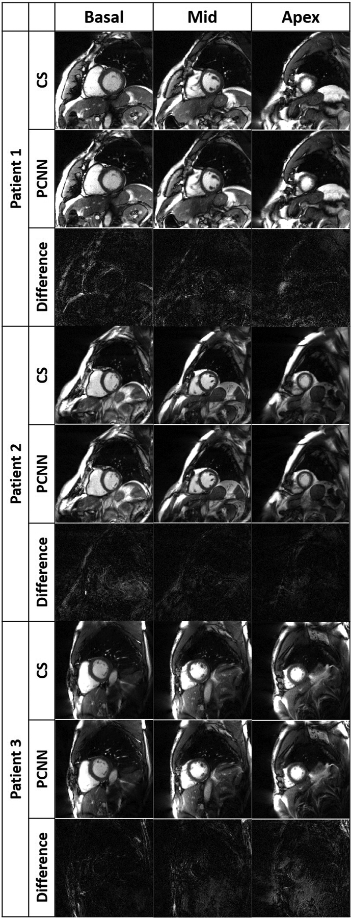
Representative images of three different patients reconstructed with CS (top row per patient), PCNN (middle row per patient), and difference image (bottom row per patient) displayed with 4-times narrow grayscale to bring out differences: basal plane (left column), mid-ventricular plane (middle column), and apical plane (right column). For dynamic display, see Videos S2–4 in Supplemental Materials.

Summarizing the result over twenty patients (see Table 2), compared with CS, the PCNN produced the best image quality metrics (SSIM = 0.88 ± 0.02, NRMSE = 0.014 ± 0.004), significantly (P<0.05) better than the magnitude and complex networks (SSIM < 0.75, NRMSE > 0.020). Relative to CS, the blur metrics were not significantly (P>0.05) different for the magnitude network and PCNN, whereas they were significantly (P<0.05) lower for the zero-filled and complex network. Given that PCNN produce the best results in two out of three categories, we elected to use PCNN throughout.

Table 2:

Summary of quantitative metrics (N=20). NRMSE and SSIM for zero-filled input images and reconstruction results by three different networks compared to CS reference.

	CS Reference	Zero-filled	Magnitude	Complex	PCNN
NRMSE		0.082 ± 0.011	0.025 ± 0.005*	0.020 ± 0.006*	0.014 ± 0.004
SSIM		0.232 ± 0.025	0.663 ± 0.056	0.742 ± 0.069	0.884 ± 0.023
Blur Metric	0.338 ± 0.015+∈	0.188 ± 0.008	0.340 ± 0.017+#	0.314 ± 0.019	0.337 ± 0.013∈#

For NRMSE and SSIM, *P > 0.05 corresponds to non-significant difference in pair. For blur metric, ^+∈#P > 0.05 corresponds to non-significant difference in pair. Note, the blur metric scores for the zero-filled and complex network with MSE loss term only reconstructions are artificially better, because they contained substantial amount of streaking artifacts which have sharp edges.

Figure 5 shows representative images of three patients reconstructed with PCNN and CS, highlighting similar image quality. For dynamic display of images shown in Figure 5, see Videos S2–4 in Supplemental Materials. Table 3 summarizes average reader scores for CS and PCNN. While all the scores were significantly different (P<0.05) between the two groups, all individual visual scores and SVS were well above the clinically acceptable cut points 3.0 and 12.0, respectively.

Table 3:

Summary of average reader visual scores. Reported values represent median and 25^th to 75^th percentiles (parenthesis).

	CS	PCNN
Myocardial Edge Definition	5.0* (4.5–5.0)	4.5* (4.0–4.5)
Temporal Fidelity	4.75* (4.5–5.0)	4.0* (3.5–4.5)
Artifacts Level	4.5* (4.0–5.0)	4.25* (4.0–4.5)
Noise Level	4.5* (4.5–5.0)	4.5* (4.0–4.5)
SVS	18.75* (17.5–19.5)	17.0* (16.0–18.0)

^*P < 0.05 corresponds to significant difference.

Figure 6 shows scatter plots resulting from linear regression analysis illustrating strong correlation between CS and DL analyses (R² ≥ 0.92) and between repeated DL analyses (R² ≥ 0.93) for all four LV functional categories. Figure 7 shows Bland-Altman plots illustrating good agreement between CS and DL analyses for LVEDV (mean =98.0mL; mean difference = −0.54 mL [0.5% relative to mean], the limits of agreement [LOA] = 14.5 mL [14.8% relative to mean]), LVESV (mean = 38.6 mL; mean difference =1.0 mL [2.6% relative to mean]; LOA = 11.3 mL [29.3% relative to mean]), LVSV (mean = 59.4 mL; mean difference = −1.6 mL [2.6% relative to mean]; LOA = 14.9 mL [25.0% relative to mean]), and LVEF (mean = 61.6%; mean difference = −1.4 % [2.3% relative to mean]; LOA = 10.9% [17.6% relative to mean]). Figure 7 also shows good agreement between repeated DL analyses for LVEDV (mean difference = −0.9 mL [0.9% relative to mean]; LOA = 8.7 mL [8.9% relative to mean]), LVESV (mean difference = 0.9 mL [2.4% relative to mean]; LOA = 10.3 mL [26.0% relative to mean]), LVSV (mean difference = −1.8 mL [3.2% relative to mean]; LOA = 9.3 mL [16.0% relative to mean]), and LVEF (mean difference = −1.4 % [2.3% relative to mean]; LOA =10.0% [16.7% relative to mean].

Figure 6:

Linear regression plots illustrating strong correlation between reconstruction methods (top row, CS vs. DL, R² ≥ 0.92) and between repeated DL analyses (bottom row, R² ≥ 0.93) for all four LV functional parameters.

Figure 7.

Bland-Altman plots illustrating good agreement between reconstruction methods (top row, CS vs. DL) and between repeated DL analyses (bottom row) for all four LV functional parameters.

Discussion

This study describes the implementation of a rapid DL reconstruction pipeline for faster (25 s per slice with 80 frames) reconstruction of non-Cartesian real-time cine complex data than GPU-accelerated CS (2:40 min per slice with 80 frames), without significant loss in image quality metrics (SSIM = 0. 88 ± 0.02, NRMSE = 0.014 ± 0.004), SVS, or LV functional parameters. By optimally learning different information contained in the real and imaginary parts of complex data and adding a perceptual loss term to suppress incoherent image features, the proposed PCNN outperformed other two architectures (magnitude with MSE loss term alone, complex network with MSE loss term alone) and successfully produced clinically acceptable image quality. Our engineering approach is based on MR physics, where the real and imaginary components contain correlated and uncorrelated (noise) information detected using a quadrature radio-frequency receiver system. Therefore, learning image features in both real and imaginary components enables more faithful image reconstruction than magnitude learning only. While the MSE loss is commonly used in DL image reconstruction, it may produce perceptually incoherent image details. By taking the perceptual loss into account, our PCNN produced better image quality compared to complex network with MSE loss term alone.

This study compares and contrasts with prior proof-of-concept DL studies for reconstructing real-time cine MR data (18, 19) as follows. The study by Schlemper et al. (18) used a cascade of convolutional neural networks (CNN)s to train on retrospectively undersampled Cartesian k-space cine data derived from fully sampled raw k-space acquired during breath-holding. The strengths of this study are that it incorporated a k-space data fidelity term and maintained multi-coil information to ensure faithful reconstruction. This study, however, had the following limitations: (a) data from only 10 patients in total (5 for training and 5 for testing); (b) did not evaluate performance on non-Cartesian k-space data; (c) the network did not learn respiratory motion because training data were acquired during breath-holding; (d) achieved good results up to 9-fold acceleration. The study by Hauptmann et al. (19) used a residual U-Net to train on synthetically undersampled non-Cartesian k-space data derived from magnitude (i.e. Digital Imaging and Communications in Medicine [DICOM]) images acquired during breath-holding. The strength of this study is that testing was evaluated on zero-filled images derived from prospectively acquired 13-fold accelerated radial k-space data. This study, however, had the following limitations: (a) deriving synthetic radial undersampled k-space data from DICOM (magnitude) files is analytically incorrect, since the signal phase information is lost following the magnitude operation; (b) the network did not learn respiratory motion because training data were obtained during breath-holding; (c) testing data from only 10 patients; (d) dealiasing performed on coil-combined, zero-filled magnitude images.

This study has several interesting points worth emphasizing. First, the proposed PCNN avoids complex value calculation that is not officially supported by Pytorch and minimizes loss of information when performing a magnitude operation to complex images. Our method provides an engineering solution to the current challenge of complex value optimization with CNNs. Second, both complex networks outperformed the magnitude network. This may be because of the fact that real and imaging components contain both correlated and uncorrelated (noise) image contents (Figure 1). Third, we used a GPU-based NUFFT in the pre-processing step to accelerate the gridding process. Despite best efforts, the pre-processing steps including gradient delay correction, gridding, and coil combination (23.7 s) was 29 times longer than the CNN filtering time (0.82 s). A future study is warranted to implement a more efficient NUFFT in Pytorch (https://github.com/mmuckley/torchkbnufft) to further reduce the pre-processing time. Fourth, the proposed PCNN pipeline produced clinically acceptable image quality, despite not having a k-space data fidelity term, by optimally learning both imaginary and real components and incorporating both MSE and perceptual loss terms. This is an efficient strategy for faithfully reconstructing non-Cartesian data, because performing NUFFT would undoubtedly slow down the processing. Fifth, while the blur metric appears to be better for zero-filled and complex network with MSE loss term only reconstructions, those scores were artificially boosted by substantial amount of streaking artifacts. Thus, the blur metric values for those two reconstructions need to be interpreted with caution. Sixth, we used the industry standard L2-loss to train our network. Several studies have shown that L-1 loss may produce better results than L2-loss (40–42). A future study is warranted to compare the performance between L-1 vs. L-2 loss functions for training our data with PCNN. Seventh, PCNN was trained on CS as reference. As such, it was not designed to outperform CS in terms image quality, but to outperform CS in terms of computational speed.

This study has several limitations that warrant further discussion. First, we used CS reconstructed real-time cine images as practical ground truth, because it was not possible to obtain fully sampled data in patients with AF. On one hand, we do not have access to ground truth, so the best we can do is treat CS reconstructions as ground truth. On the other hand we have demonstrated a NN implementation that we can confidently say has successfully learned the CS algorithm, as verified by the results and analysis presented in this paper. Second, we did not incorporate a k-space data consistency term into our model because NUFFT and inverse-NUFFT are time consuming operations for non-Cartesian data. Another practical reason for not including a data consistency layer is GPU memory requirement, since such an operation would also necessitate multi-coil information. A future study is warranted to incorporate a data consistency layer for non-Cartesian data using a GPU server with very high memory capacity. Third, our training (multi-slice 2D+time) data were obtained from twenty patients. While the total number of patients may appear to be small, we used 31,840 2D images (or 1,173,749,760 voxels) and 2,547,072 parameters for PCNN for paired supervised learning with 3 × 3 × 3 kernels. Note, our training data size (twenty patients) is at least 4 times larger than the training data size (5 patients) used by Schlemper et al. (18). Fourth, while PCNN produced clinically acceptable visual scores for all four individual categories, its lowest score was temporal fidelity of myocardial wall motion. Subtle blurring of myocardial wall motion was visible in some slices, which may have contributed to small (1.4%) underestimation in LVEF. Fifth, we designed PCNN based on a U-Net. It may be possible to achieve better results using more sophisticated unrolled network architectures (42, 43) with more powerful GPU and more training data, at the expense of greater computational demand and processing time. From a practical point of view, fast processing is essential for our clinical application, and access to a high-end GPU server with very high memory may be limited at most centers. Nonetheless, a future study is warranted to compare the performance between the proposed PCNN and more sophisticated networks.

In summary, this study describes implementation, training, and testing of an image reconstruction pipeline including a PCNN architecture for faster reconstruction of non-Cartesian real-time cine complex MR data than GPU-accelerated CS reconstruction, without significant loss in quantitative metrics of image quality, SVS, or LV functional parameters, thereby verifying clinical translatability.

Supplementary Material

VideoS4

Supplementary Video S4. Dynamic display of the CS (top row) and PCNN (bottom row) reconstructed images of patient 3 shown in Figure 5.

VideoS2

Supplementary Video S2. Dynamic display of the CS (top row) and PCNN (bottom row) reconstructed images of patient 1 shown in Figure 5.

VideoS3

Supplementary Video S3. Dynamic display of the CS (top row) and PCNN (bottom row) reconstructed images of patient 2 shown in Figure 5.

VideoS1

Supplementary Video S1. Dynamic display of the images (top row) shown in Figure 4.

FigureS1

Visual display of features extracted from VGG-16 network for CS and DL. 8 out of 256 feature maps were randomly selected and shown on the right.

List of Abbreviations

b-SSFP

balanced steady-state free precession

CNN

convolutional neural network

CS

compressed sensing

CV

coefficient of variation

DL

deep learning

DICOM

Digital Imaging and Communications in Medicine

FOV

field of view

GPU

graphic processing unit

HIPPA

Health Insurance Portability and Accountability Act

LOA

limits of agreement

LV

left ventricular

LVEDV

left ventricular end-diastolic volume

LVEF

left ventricular ejection fraction

LVESV

left ventricular end-systolic volume

LVSV

left ventricular stroke volume

MSE

mean squared error

NRMSE

normalized root mean squared error

NUFFT

Non-Uniform Fast Fourier Transform

PCNN

perceptual complex neural network

ReLU

rectified linear unit

RING

Radial Intersections

SSIM

structural similarity index

SVS

summed visual scores

VGG

Visual Geometry Group