

Summary.
It is common in the analysis of social network data to assume a census of the networked population of interest. Often the observations are subject to partial observation due to a known sampling or unknown missing data mechanism. However, most social network analysis ignores the problem of missing data by including only actors with complete observations. In this paper we address the modeling of networks with missing data, developing previous ideas in missing data, network modeling, and network sampling. We use several methods including the mean value parameterization to show the quantitative and substantive differences between naive and principled modeling approaches. We also develop goodness-of-fit techniques to better understand model fit. The ideas are motivated by an analysis of a friendship network from the National Longitudinal Study of Adolescent Health.
1. Introduction
Social network data typically consist of a set of n actors and a relational variable Yi,j, measured on each ordered pair (i, j), i, j = 1, …, n. We focus on binary relations, for which Yi,j is a dichotomous variable indicating the presence or absence of some relation of interest, such as communication, friendship, etc. The data Y = {Yi,j}i≠j can be thought of as a graph in which the nodes are actors and the edge set is {(i, j) : Yi,j = 1}. We consider a case where some Yi,j are unobserved due to out-of-design missingness. The analyses in this paper are concerned with characterizing the structure of friendships among high school students, measured as part of the National Longitudinal Study of Adolescent Health (Add Health, Harris et al. (2003)).
1.1. The National Longitudinal Study of Adolescent Health
Add Health is a school-based, longitudinal study of the health-related behaviors of adolescents and their outcomes in young adulthood. The study design sampled 80 high schools and 52 middle schools from the US, representative with respect to region of country, urbanicity, school size, school type, and ethnicity (Harris et al., 2003). In 1994–95 an in-school questionnaire was administered to a nationally representative sample of students in grades 7 through 12. In addition to demographic and contextual information, each respondent was asked to nominate up to five boys and five girls within the school whom they regarded as their best friends. Thus each student could nominate up to ten students within the school (Udry, 2003). This referral structure results in directed network data, where an arc or directed tie is said to exist from node i to node j if and only if i named j a friend. We define “friend” to be one of a student’s top five male or top five female friends, and conduct all our analyses restricting networks and models to networks constrained by this definition. There is an extensive and growing literature describing and utilizing the Add Health survey - see the cites of Resnick et al. (1997) and Udry and Bearman (1998) for a bibliography and more information.
We have selected one school, School 5, for our analysis. Seventy students from this school completed the friendship nominations portion of the survey. From later waves of the survey, we were able to recover the sex and grade of 19 additional students who did not supply their friendship nominations in the original survey. In this section we consider the friendship nominations among these 89 students to be the focus of scientific interest. In particular we are interested in inferring the social process that generated the observed set of friendship arcs among the 89 students. Of these, 70 reported arcs and 19 did not report arcs. Thus our data contain known arcs and non-arcs between the 70 students who completed surveys, and known arcs sent by the 70 respondents to the 19 non-respondents. They do not include information on arcs among the 19 students who did not complete surveys or sent by the non-respondents to the respondents. Hence of the 7832 potential nominations 19 × 88 = 1672, or 21% were unobserved. These missing arcs due to survey non-response constitute the missing data we are concerned with.
The structure of the relations is usually dependent on the attributes of the actors. For example, for most social relations the likelihood of a relationship is a function of the age, gender, geography and race of the individuals. Homophily on attributes, or the tendency for like to share ties with like, is a common example (McPherson, Smith-Lovin, and Cook, 2001). In the adolescent friendships in our application, the social structure is highly dependent on class grade (grades 7–12) and sex. In addition to exogenous attributes of the actors, relationships are influenced by endogenous attributes such as their positions in the network (White, Boorman, and Breiger 1976). In the Add Health data, we are particularly interested in examining the hierarchal or egalitarian structures of the friendship nominations, which we study using endogenous structures.
1.2. Modelling Networks with Missing Data
In this paper we consider the network over the set of actors to be the realization of a stochastic process and model the process. The statistical modeling of such processes has a long history. Holland and Leinhardt (1981) appear to be the first to propose log-linear models for social networks. Their models resulted in each dyad — by which we mean each pair of actors — having edges independently of every other dyad. Frank and Strauss (1986) generalized to the case in which dyads exhibit a form of Markovian dependence: Two dyads are dependent, conditional on the rest of the graph, only when they share a node. Such exponentially parametrized random graph models have connections to a broad array of literatures in many fields, such as spatial statistics, statistical exponential families, and statistical physics (Geyer and Thompson, 1992). Since that time there have been many theoretical and applied developments (Lusher et al., 2012).
The analysis of sampled or missing data in networks is special for two reasons. First, we are often interested in models in which variables on all units of analysis are dependent. Thus instead of inference from multiple independent observations of a given process, standard network modeling is based on a single observation of a dependent process. In this way, network modeling is similar to time series modeling. When the network is only partially-observed, inference must therefore be conducted on a single partially-observed realization of the process. Second, networks consist of two fundamental units: nodes and dyads. In our framework, we consider the dyadic relations to be stochastic, and the simplest units of inference. Sampling and missing data processes, however, often act on the nodes, as much network data is collected through egocentric reporting processes (e.g., people reporting their own relations). Therefore, the units of inference reside between the units of observation. This is the pattern observed in our application, where missing friendships result from some students not completing the survey. Thus data are missing in highly dependent blocks, where all nominations of each non-respondent are unobserved.
Many practical settings result in missing network data. In this paper, we address what is perhaps the most common pattern: when dyads are observed through their incident nodes, and an attempted census of network nodes fails to reach some nodes, leaving some dyads unobserved. In human social networks including the Add Health study, such non-observation could be due to response refusal, absence, or illness. Other forms of missing data in networks may result from non-observation of individual dyads or of nodal covariates. Despite the general acceptance that missing data is an important problem for social network analysis, there has been little work on inferential frameworks to treat social networks with missing data.
Some approaches to model-based treatment of missing data in social networks have been suggested, but due to the difficulty of the problem, they typically rely on special cases and assumptions. Stork and Richards (1992) advocate leveraging the strong effect of reciprocity in many networks to impute missing arcs, or directed edges, in directed networks by setting them equal to their opposite arcs, such that if the relation from j to i is unobserved, it is set equal to the relation from i to j whenever the latter is observed. This approach is often more reasonable than treating the arc from j to i as a known non-arc, but is not ideal for several reasons. First, as Stork and Richards point out, the approach is only valid for directed networks with very strong reciprocity. When reciprocity is not so strong (i nominating j does not strongly predict j nominating i), this approach may perform worse than pretending the reciprocating arcs do not exist. This approach also treats the newly imputed arcs as true, rather than treating them probabilistically. In addition, this approach does not address the arcs that may originate from the missing actors which are not reciprocated, or any arcs between missing actors.
The first model-based approach to networks with missing data was introduced by Robins et al. (2004), who use an exponential family model with the maximum pseudo-likelihood estimates (MPLE) of the parameters based on treating arcs between respondents and other respondents separately from arcs from respondents to non-respondents. This approach is most helpful if it is known that the arc-related characteristics of non-respondents are different from those of respondents in ways that are not captured in the terms in the model. However, it does not allow for the consideration of network structures which span the boundary between observed and unobserved parts of the network, or allow for models applicable to the full populations of possible arcs. There is also evidence that the MPLE performs poorly for realistic network structures (van Duijn et al., 2009).
The most systematic treatment of missing data in networks to date is provided by Koskinen et al. (2013). They consider a Bayesian approach for missing tie variables and covariates, allowing for inference based on the full posterior of the parameters, as well as predictive inference for the unobserved parts of the network.
Our companion paper, Handcock and Gile (2010), building on Thompson and Frank (2000), develops a likelihood-based framework for the full-network modeling of networks that are partially-observed due to sampling. In this paper, we use the likelihood-based approach of Handcock and Gile (2010) and Koskinen et al. (2013) while focusing on broader issues of data analysis, including goodness-of-fit diagnostics and leveraging the network data structure to address systematic patterns of missing data.
It is also worth mentioning a related area of research: techniques for sharing social network data that protect sensitive personal information privacy while retaining key statistical information. Karwa et al. (2014) and Karwa et al. (2015) develop an approach to share synthetic networks with perturbed ties where the perturbation mechanism is carefully designed by the researcher to meet these differentially privacy goals. Their statistical techniques are similar in approach to those developed by Handcock and Gile (2010) and this paper. The problem is substantially different, however, in that the perturbation mechanism is fully known while none of the data elements are known with certainty.
Following this introduction, in Section 2, we introduce several types of missing data in social networks. In Section 3, we review the general principles involved in fitting models to social networks with missing data. Section 4 introduces the widely-used and powerful exponential family random graph model (ERGM) class for networks, and discusses the fitting of these models for networks with missing data. The approaches in this section are available in the statnet R package (Handcock et al., 2003).
Finally, we use these theoretical pieces to present an analysis of adolescent friendship data in Section 5, including the introduction of several descriptive and diagnostic approaches for partially-observed network data. We finish with a discussion.
2. Missing Data Structures
We treat missing data as a special case of sampling in which the sampling mechanism is unknown and outside the control of the researcher, or an out-of-design non-response mechanism. As in the companion paper focused on sampling (Handcock and Gile, 2010), we use the N-vector S to indicate the observed status of each node, and the N ×N matrix D to represent the observed status of each directed dyad, such that.
| (1) |
We focus on the situation where the sampling design specifies S = 1 and Dij = 1 for all i ≠ j, that is, the researchers intended to observe all nodes and relations. In the case of missing data, however, the observed values of S and D are jointly determined by the sampling and missing data mechanisms, such that Dij = 0 for some i ≠ j. In this section, we explicitly describe several possible missing data mechanisms.
2.1. Non-responding nodes
It is often the case that a census of the network is attempted via a complete census of the nodes followed by the observation of all edges incident to each node. This is the case, for example, in networks between people where each person, is asked to report her relations to all others in the network, a sampling design corresponding to a nodal census. However if some nodes do not respond, many ties variables will be missing. In an undirected network in which we observe all dyads incident to each observed node,
For a directed network in which we observe all dyads originating at an observed node, D = S1T. Note that both of these mappings are identical to the case of sampling considered in Handcock and Gile (2010). Unlike in the case of sampling, the missing data mechanism ϕ is typically unknown, even up to a model class. In the simplest case, we might consider a missing data mechanism corresponding to a simple random sample of nodes whereby
More complex mechanisms include functions depending on nodal characteristics or observed network features, or those depending on unobserved features. Such missing data structures can also result from link-tracing designs, where the intention is to sample the contacts of all previously sampled nodes, but the referral and contact process does not reach each contact. Note that when this structure is by design, as in partial-wave link tracing samples, the data are not missing.
2.2. Unobserved (Directed) Dyads
Particular dyads or directed pairs may also be unobserved, even if their incident nodes are observed. A particularly difficult form of this pattern is when some edges are observed, but few or no non-edges are observed. This is often the case in protein interaction networks, where published papers tend to report observed protein interactions, but not tests for interaction with negative results.
2.3. Partially-Observed Nodal Attributes
Often, observing a node implies observation of associated nodal covariate information, as in self-report surveys. There is also sometimes non-response on individual items, even for observed nodes. It is also possible that nodal covariate information is available even for nodes that are not sampled, as in administrative databases on well-defined populations.
2.4. Boundary Specification
All of the examples thus far assume the set of actors is well-defined and the number of actors in the population is known. It is often the case that it is unclear which nodes should be considered part of the population of interest. Such cases are beyond the realm of models currently in standard use, and also beyond the scope of this paper. In our analyses, we assume that we know the exact set of nodes in the network, but that some of the dyads are unobserved.
2.5. Frameworks for Analysis
We focus on two strategies for inference, which we refer to as complete case and all observations analysis. In complete case (CC) analysis, only nodes with fully-observed data are considered. This approach is also referred to as subnet analysis, as in this case, only the subnet induced by the nodes with full available information is analyzed. The advantage of this approach is that is does not require any special software for missing data. However, it ignores both the larger size of the full network to which we wish to apply a model, as well as any additional information available on the cases that are not complete. Shalizi and Rinaldo (2013) show that analyses based on subnetworks cannot be consistently applied to the true larger network, so this naive approach is not statistically principled. Therefore, researchers interested in finding a principled model fit for the true full network, and interested in using all available data should prefer the more principled approach, which we call the all observations (AO) approach. In this approach, all available data are used in the analysis, including all observed relations, the population size, and all known nodal characteristics. The majority of our paper treats these two inferential approaches, and compares the resulting model fits, as these are the approaches most likely to be employed in practice.
We also include two more specialized model fits. First, for comparison, we also consider an incomplete case (IC) approach, which fits a model over the full known size and nodal covariates of the network, but treating all dyads involving non-respondents as unobserved. This fit helps us distinguish the separate impacts of the additional data and the larger network size on the differences between CC and AO fits. Finally, we apply a differential popularity (DP) analysis to directly model observed systematic differences between respondents and non-respondents in our data, in partial adjustment for irregularities in the missing data process.
3. Principled Likelihood Inference for Partially-Observed Networks
Our development here follows the development in the companion paper Handcock and Gile (2010), which follows Little and Rubin (2002) and Thompson and Frank (2000). For most of this treatment, we consider the case of fully-observed covariates information, X. Consider a parametric model for the random relational matrix Y, depending on a parameter p–vector η and an N × q matrix of nodal covariates X:
| (2) |
where Ξ is the space of possible parameter values η and is the set of possible networks on the n actors with covariates X = x. In the model-based framework, if Y and X are completely observed inference for η can be based on the likelihood:
This situation has been considered in detail in Hunter and Handcock (2006) and the references therein. In the general case where Y may be only partially observed, we denote the observed part of Y by Yobs = {Yij : Dij = 1} and the unobserved part by Ymis = {Yij : Dij = 0}, then Y = {Yobs, Ymis}. The complete data, {Yobs, Ymis, D}, are not fully observed, and the observed data are {Yobs, D}. Following Handcock and Gile (2010), we make the convention that undefined numbers act as identity elements in addition and multiplication, such that Y = Yobs + Ymis. Letting lower-case symbols represent the observed values of random variables, we let represent the set of possible values of Ymis, consistent with yobs. Then is the subset of consistent with yobs.
If the missing data mechanism is missing at random (MAR, Rubin 1976), in the sense that:
| (3) |
and the parameters ψ and η are distinct, then the likelihood for η and ψ is
Thus likelihood-based inference for η from L[η, ψ|Yobs, D, X = x] will be the same as based inference for η based on L[η|Yobs, X = x]. The latter is typically easier:
Hence we can evaluate the likelihood by just enumerating the full data likelihood over all ues for the missing data.
4. Exponential-family Random Graph Models
We model the random behavior of Y using an exponential-family random graph model. The standard exponential family model form is:
| (4) |
where Z(Y) is a p-vector of statistics, η ∈ Rp is a parameter vector, and is the normalizing constant (Barndorff-Nielsen, 1978).
There is a wide range of network statistics that could be included in Z(y|X = x) (Lusher et al., 2012). In the network modeling literature these are referred to as exponential-family random graph models or ERGMs (Hunter and Handcock, 2006). We allow the vector Z(y|X = x) to include covariate information about nodes or dyads in the network in addition to information derived directly from the matrix y itself.
In a sampling-focused companion paper, we address the fitting of ERGMs for partially-observed network data with a MAR structure (Handcock and Gile, 2010) using a natural extension of this method. Consider that
| (5) |
where is the normalizing constant of the conditional distribution of Ymis|Yobs, X = x:
| (6) |
To find the MLE, we therefore maximize an estimate of (5) computed as the ratio of the two normalizing constants. The exp[κ(η, x)] term is estimated using unconditional samples of Y, as in standard ERGM model fits, while exp[κ(η|yobs, x)] is estimated by conditionally sampling from Ymis|Yobs and X = x according to (6) (Geyer and Thompson, 1992; Hunter and Handcock, 2006). This is implemented in the statnet R package (Handcock et al., 2003).
5. Analysing Adolescent Friendship Networks
We consider four modeling approaches for the Add Health adolescent friendship network with missing data. We begin by describing the pattern of missing data. We then introduce the common model used in all the approaches. We next compare the approach presented in Section 4 to a naive approach, modeling the subnetwork consisting of respondents only (a complete case approach), and use several methods to estimate the magnitude of the difference between the two approaches. We illuminate both numerical and substantive differences. We illustrate some diagnostic procedures for partially testing the missing-at-random assumption, and introduce a third modeling approach partially correcting for the failure of the missing-at-random assumption. We also include a fourth modeling approach to explain some differences between the first two.
5.1. Missing Data Pattern
The data pattern is shown in Figure 1. Consider a partition of respondents from non-respondents and the corresponding 2 × 2 blocking of the sociomatrix, with the four blocks representing arcs from respondents and non-respondents to respondents and non-respondents. The complete data consists of the full sociomatrix. The first two blocks contain the observed data (the arcs sent by respondents), and the second two blocks contain the unobserved data (those sent by non-respondents).
Fig. 1:
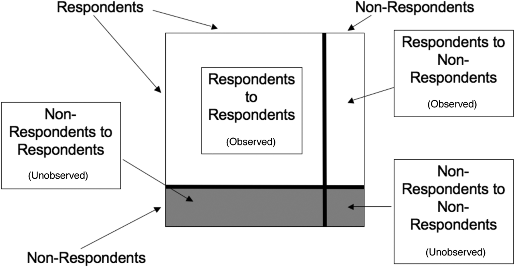
Schematic depiction of observed and unobserved arc data.
Almost all analysis of the Add Health network data uses the complete case approach, treating the network among the respondents only, excluding those who did not complete the survey (Bearman et al., 2004; Harris et al., 2003), and corresponding to considering only the upper left hand block of Figure 1. We can also visualize the excluded data by plotting the network both including and excluding the non-respondents, then plotting only the arcs to non-respondents as in Figure 2. For clarity, the positions of the nodes are the same in each plot.
Fig. 2:

A depiction of the data excluded by the complete case analysis. (a) depicts all of the observed data. (b) only the relations between respondents, the data considered in a complete case analysis, and (c) depicts the difference. The positions of the nodes are the same in each subplot. Node color represents grade and shape represents sex (female=square). The grades are 7=red, 8=turquoise, 9=purple, 10=green, 11=blue, 12=black.
5.2. Model Specification
We specify an ERG model for the social process in which g(y, X), the set of network statistics has twenty-one terms. The first term, named density, captures the overall tendency for edges in the network. The corresponding sufficient statistic is the total number of arcs: ∑i≠j yij. In an ERGM, this term has a role similar to the intercept in a regression model. The next term, Mutuality, captures the tendency for arcs to be reciprocated, and has sufficient statistic ∑i<j yijyji. The next seven terms capture the differential tendency for nodes of different classes to receive arcs. Grade 7 females serve as the reference category. The additional tendency for Grade 8 females to receive arcs is given by the Grade 8 Popularity term with sufficient statistic:
| (7) |
where is the the indicator function taking the value 1 when k is true, and 0 otherwise. The remainder of the grade popularity terms are defined similarly, and the Male Popularity term has sufficient statistic
| (8) |
We leave the definition of the Non-Respondent Popularity term to Section 5.5.
The Sex and Grade Mixing terms capture the differential tendencies for arcs across sex and grade classes, and respects the potentially asymmetrical patterns of these relations. The Girl to Same Grade Boy term has sufficient statistic
| (9) |
and captures the differential tendency for female students to send arcs to males in the same grade, against the reference of females in the same grade. The Boy to Same Grade Girl term is similarly defined.
The remaining terms in this set capture linear functions of grade differences. For example, the Girl to Older Girl term has sufficient statistic
| (10) |
such that the corresponding parameter indicates the change in tendency for arcs corresponding to each one-grade difference between two female students. This parameterization assumes that each one year difference in grade has the same impact on friendship formation. The remainder of the terms in this section are similarly defined.
The Transitivity terms are a measure of hierarchy or equality in social networks. Having captured the hierarchical tendencies across sex and grade in the Sex and Grade Mixing terms, here, we consider the Transitivity effects within sex and grade only. The Transitive Same Sex and Grade term is based on transitive triad structures. If arcs are sent in an hierarchical manner, then if B names A (making A above B), and C names B (making B above C), then the triad is likely to be completed in a transitive manner with C naming A, since by transitivity A would be above C. The sufficient statistic capturing this structure is
| (11) |
Similarly, a cyclical triad structure is indicative of an egalitarian relational structure. Here, B → A and C → B make A, B, and C about equal, making cyclical triadic completion (A → C) likely. These structures are captured with sufficient statistic
| (12) |
The final term, Isolation, captures the tendency for some nodes to receive no friendship nominations, beyond what would be expected given the rest of the terms in the model. This term is based on sufficient statistic
| (13) |
We estimate the MLE of the parameters of this model conditional on the restriction in the data that no node may nominate more than five female friends or five male friends.
5.3. Model Fit
The parameter estimates under the all observations approach are summarized in the first and fifth columns of Table 1. All terms are nominally significant at the .01 level except the terms capturing the differential popularity by grade and sex, and the terms comparing cross-sex and within-sex popularity within the same grade. Ninth and tenth graders and males do show nominally significant differences in popularity at the .05 level. This fit supports several scientific hypotheses about the social mechanisms giving rise to this observed network.
Table 1:
Estimated coefficients and standard errors for the parameters of the model fits under the All Observations (AO), Complete Case (CC), Differential Popularity (DP), and Incomplete Case (IC) approaches.
| AO | CC | DP | IC | AO s.e. | CC s.e. | DP s.e. | IC s.e. | |
|---|---|---|---|---|---|---|---|---|
| Density | −1.929 | −1.557 | −1.901 | −1.923 | 0.19*** | 0.19*** | 0.19*** | 0.20*** |
| Mutuality | 1.728 | 1.963 | 1.726 | 1.854 | 0.19*** | 0.20*** | 0.19*** | 0.21*** |
| Sex and Grade Factors | ||||||||
| Grade 8 Popularity | −0.161 | −0.218 | −0.144 | −0.402 | 0.12 | 0.12 | 0.12 | 0.15** |
| Grade 9 Popularity | −0.301 | −0.330 | −0.324 | −0.353 | 0.14* | 0.14* | 0.14* | 0.16* |
| Grade 10 Popularity | −0.318 | −0.277 | −0.303 | −0.374 | 0.14* | 0.14* | 0.14* | 0.16* |
| Grade 11 Popularity | −0.043 | −0.033 | 0.027 | −0.042 | 0.17 | 0.18 | 0.18 | 0.24 |
| Grade 12 Popularity | −0.095 | 0.062 | −0.010 | −0.175 | 0.16 | 0.17 | 0.16 | 0.20 |
| Male Popularity | 0.407 | 0.461 | 0.452 | 0.504 | 0.16* | 0.16** | 0.16** | 0.21* |
| Sex and Grade Mixing | ||||||||
| Non-Resp Popularity | - | - | −0.313 | - | - | - | 0.12** | - |
| Girl to Same Grade Boy | 0.193 | 0.001 | 0.175 | 0.074 | 0.21 | 0.23 | 0.22 | 0.29 |
| Boy to Same Grade Girl | −0.217 | −0.155 | −0.231 | −0.078 | 0.22 | 0.23 | 0.21 | 0.25 |
| Girl to Older Girl | −0.956 | −0.959 | −0.962 | −1.115 | 0.16*** | 0.18*** | 0.16*** | 0.23*** |
| Girl to Younger Girl | −1.318 | −1.308 | −1.334 | −1.340 | 0.21*** | 0.21*** | 0.21*** | 0.25*** |
| Girl to Older Boy | −0.901 | −1.066 | −0.906 | −1.069 | 0.14*** | 0.17*** | 0.14*** | 0.20*** |
| Girl to Younger Boy | −1.326 | −1.375 | −1.339 | −1.894 | 0.22*** | 0.23*** | 0.22*** | 0.38*** |
| Boy to Older Boy | −0.876 | −1.137 | −0.885 | −0.943 | 0.15*** | 0.21*** | 0.15*** | 0.22*** |
| Boy to Younger Boy | −1.789 | −2.082 | −1.807 | −2.696 | 0.33*** | 0.40*** | 0.33*** | 0.71*** |
| Boy to Older Girl | −0.680 | −0.521 | −0.683 | −0.533 | 0.14*** | 0.14*** | 0.14*** | 0.16*** |
| Boy to Younger Girl | −1.114 | −1.048 | −1.125 | −0.959 | 0.17*** | 0.17*** | 0.17*** | 0.17*** |
| Transitivity | ||||||||
| Transitive Same Sex and Grade | 0.502 | 0.502 | 0.497 | 0.477 | 0.05*** | 0.06*** | 0.05*** | 0.05*** |
| Cyclical Same Sex and Grade | −0.913 | −0.995 | −0.891 | −0.865 | 0.18*** | 0.20*** | 0.18*** | 0.21*** |
| Isolation | 2.664 | 3.059 | 2.355 | 3.617 | 0.90*** | 0.62*** | 0.94*** | 0.71*** |
= p < .05,
= p < .01,
= p < .001
First, friendship arcs are reciprocated at a higher rate than we would expect at random given the other terms in the model. With regard to grade, 9th and 10th graders receive significantly fewer friendship nominations than the reference 7th graders, although this finding is weaker than the others.
Males receive within-sex nominations at a nominally higher rate than females. Both males and females seem less likely to nominate friends outside their grades, with the chance of nomination decreasing with the number of class years. Looking at the effect sizes for the Sex and Grade Mixing terms together, we note that, although not significant, boys show a stronger aversion to sending cross-sex nominations within grade. We also see that both sexes appear more likely to nominate older (higher grade) rather than younger (lower grade) friends. This effect is stronger in males, with a particularly strong prohibition against males nominating younger males as friends.
The positive significant transitive triad, and negative significant cyclical triad terms suggest that friendship arcs within sex and grade tend to form in an hierarchical manner, rather than in an egalitarian regime. This finding is likely the most scientifically interesting of the processes supported by this model.
Finally, arcs are clustered so as to produce more nodes receiving no friendship nominations than we would expect from the rest of the terms in the model.
Columns 2 and 6 of Table 1 presents the corresponding complete case model fit. It is of interest to compare the AO and CC models. The question here is the impact of erroneously using the CC model when the full network model is of interest. A natural way to compare the models is the Kullback-Leibler divergence of the CC model from the AO model when both are used to model the CC subnetwork. Specifically, we can consider the probability distribution that the AO model for the full network places over the CC network dyads: , and use it to compute the Kullback-Leibler divergence:
| (14) |
where is the AO model for the full network, is the CC model for the CC subnetwork and YCC is the set of dyads from the full network in the CC subnetwork. The method to compute this divergence is given in the Appendix. The value of the divergence is 159. The large magnitude of this divergence indicates that the AO and CC models are substantially different representations of the CC subnetwork (Cover and Thomas, 2006).
Because the AO and CC approaches fit models to different networks, with different sets of nodes, we know from Shalizi and Rinaldo (2013) that direct comparison of the natural parameters of the two approaches is not valid: the interpretations of coefficients are different in different node-set contexts. Nonetheless, researchers often draw substantive conclusions based on the magnitudes and significances of model coefficients, so it is of interest to compare the conclusions that might be drawn by researchers using one approach or the other. At first glance, comparison of the model fits in Table 1 reveals striking similarities among the natural parameters for these two approaches. The fits find nearly identical patterns of statistical significance. A researcher basing conclusions on the sign and significance of individual model terms would draw nearly the same conclusions from either of these fits. That said, there are also notable differences in the magnitudes of coefficients. In particular, the CC fit reflects a greater popularity of 12th graders, and a greater tendency for students to receive no arcs. It also suggests a tendency for girls to send fewer arcs to same-grade boys and fewer arcs to older boys. The CC fit suggests boys are more likely to send arcs to same-grade girls, less likely to send arcs to older or younger boys, and more likely to send arcs to older girls. The interpretation of these effects is complicated by the many terms in the model. If the CC fit reflects higher overall popularity of 12th graders, do lesser estimates for terms for arcs sent to older students merely reflect that this phenomenon has already been captured by the 12th grade popularity term?
We can better compare the marginal effects of the two fits by comparing the mean value parameterizations of the two fits, as presented in Table 2.
Table 2:
Estimated mean value parameters and standard errors for the model fits under the All Observations (AO), Complete Case (CC), Differential Popularity (DP), and Incomplete Case (IC) approaches. The Density coefficient is in percent of possible ties.
| AO | CC | DP | IC | |
|---|---|---|---|---|
| Density | 7.606 | 8.158 | 8.134 | 7.245 |
| Mutuality | 77.453 | 93.990 | 86.485 | 77.168 |
| Sex and Grade Factors | ||||
| Grade 8 Popularity | 90.895 | 92.070 | 96.585 | 72.062 |
| Grade 9 Popularity | 67.230 | 71.994 | 69.218 | 66.624 |
| Grade10 Popularity | 55.296 | 61.975 | 59.456 | 53.841 |
| Grade 11 Popularity | 47.571 | 57.913 | 55.296 | 47.946 |
| Grade 12 Popularity | 33.789 | 36.097 | 38.175 | 32.159 |
| Male Popularity | 182.424 | 200.999 | 198.345 | 172.386 |
| Sex and Grade Mixing | ||||
| Girl to Same Grade Boy | 57.373 | 59.055 | 60.687 | 57.111 |
| Boy to Same Grade Girl | 39.111 | 42.027 | 41.133 | 40.263 |
| Girl to Older Girl | 21.021 | 22.017 | 22.358 | 16.073 |
| Girl to Younger Girl | 15.069 | 16.040 | 15.501 | 14.223 |
| Girl to Older Boy | 38.211 | 34.954 | 41.820 | 32.316 |
| Girl to Younger Boy | 16.595 | 19.992 | 17.771 | 9.316 |
| Boy to Older Boy | 21.301 | 18.046 | 23.371 | 19.534 |
| Boy to Younger Boy | 6.212 | 5.992 | 6.704 | 2.347 |
| Boy to Older Girl | 29.558 | 40.000 | 31.683 | 33.661 |
| Boy to Younger Girl | 22.542 | 24.019 | 23.258 | 24.964 |
| Transitivity | ||||
| Transitive Same Sex and Grade | 153.144 | 216.549 | 186.802 | 153.131 |
| Cyclical Same Sex and Grade | 35.247 | 54.847 | 45.497 | 36.800 |
| Isolation | 2.065 | 3.991 | 1.341 | 4.184 |
The mean value parameterization provides an alternative to the natural parametrization of the ERGM. The mean-value parameters are given by:
| (15) |
This parameterization puts the coefficients on the scale of the network statistics rather on the conditional log-odds scale of the natural parameters. Looking at the mean value parameters provides a sense of the implications of the model fit for the network statistics. Although we assume both models are intended to model the structure of the full network of 89 nodes, there is no principled way to directly apply this model to the larger network (Shalizi and Rinaldo, 2013). We therefore compare the models based on their mean value parameterizations applied to the portion of the network for which they each provide valid probability models: the subnetwork of 70 respondents. For the AO fit, these values are determined by marginalizing over the rest of the network. This puts both fits on the same scale to allow for meaningful comparisons.
Table 2 shows the MLEs of the mean value parameters (The complete table including their standard errors is included in the Appendix Table A1). To begin with, the expected number of arcs demonstrates that the CC fit implies about 7% more arcs (394) than the AO fit (367), and 21% more reciprocated arcs (94 vs 77). The mean value parameters of other model terms support conclusions suggested by the natural parameters. Under the CC fit, 12th graders receive more arcs (7% more), and more students receive no friendship nominations (almost twice). Differences in rates of cross-sex nominations within grade are not large. The weighted sum of arcs from girls to older boys is lower (9%). The weighted sums of arcs from boys to older and younger boys are reduced (15% and 4% respectively), and those to older girls are increased (35%). Unexpectedly, the number of transitive and cyclical triads within sex and grade are substantially higher in the CC fit (41% and 56% respectively), although the natural parameter estimates for these terms were nearly identical. Since these terms are focused on arcs within sex and grade, the observed differences are likely due to greater concentration of arcs within sex and grade for the CC fit. This phenomenon is consistent with the relatively higher rate of sex-grade homophilous arcs from respondents to respondents, as opposed to from respondents to non-respondents. Figure 3 compares the proportion of observed in-arcs received from outside one’s own sex and grade for respondents and non-respondents of the same sex and grade. Note that for six of the eight sex-grades with non-respondents, non-respondents received a higher proportion of nominations from outside their own sex and grade. The greatest exception to this pattern is 12th grade girls, for whom non-respondents receive a lower proportion of nominations from outside their sex and grade than their respondent counterparts. This is consistent with the increased rate of “boy to older girl” nominations, and decreased rate of most other arc types across sex and grade under the CC fit.
Fig. 3:

Mean proportion of nominations received from outside sex and grade, by sex and grade.
The AO approach relies on two types of information not used in the CC approach: the full size of the network, and the additional data in the arcs sent to non-respondents. To help distinguish the effects of these two differences, we fit the same model to a network of size 89 × 89 with only the respondents to respondents block observed. Columns 4 and 8 of Table 1 presents the resulting fit, which we refer to as the incomplete case (IC) fit. A naive reading of Shalizi and Rinaldo (2013) may suggest that the parameters for the full network can not be estimated by apply the model to the subnetwork data alone. As we see the parameter estimates are close to the AO case (that uses the full observed data and the same model). The same is true for the mean value parameters given in column four of Table 2. The full table, including the standard errors of the mean value parameters is given in the Appendix Table A1. These are useful as they indicate that the uncertainty in the mean value parameter estimates for the isolates is large. The Kullback-Leibler divergence of the IC model from the AO model when both are used to model the CC subnetwork is 8.4. As the corresponding divergence for the CC model is 159, this indicates that the IC fit is much closer to the AO fit then the CC fit for the CC subnetwork. This suggests that much of the difference between the AO and CC fits is due to the assumed size of the full network.
5.4. Goodness-of-Fit
Hunter et al. (2008) present a method for evaluating the fit of network models, based on network statistics not modeled directly. They propose comparing the distribution of selected statistics of substantive interest (e.g, degree distribution and shortest path length distribution) to their observed values. They draw a sample of networks from the model specified by the MLE, and compare the observed to the sampled distribution of statistics via boxplots. The closer the observed statistics are to the middle of the sample distributions, the better the fit of the model. We extend this approach to networks modeled with missing data.
When the model includes missing data, we are still interested in the features of the full network, but it is only partially observed. For this reason, we estimate the reference distribution as the network statistics based on simulations of the unobserved data conditional on the observed data under the MLE. The mean of these values are taken as the reference distribution, depicted with a solid line. Boxplots representing the distribution under the model are then added based on unconditional simulations under the MLE, as in the fully-observed data case. Figure 4 depicts three such plots for the All Observations model fit. This model reproduces the in-degree distribution quite well. It smooths some jaggedness in the out degree distribution. Also, it recovers the distribution of mean minimum geodesic distances, or the minimum number of arcs between each pair of nodes, fairly well, although it slightly under-estimates these distances. Corresponding plots for the Complete Case and Differential Popularity (to be introduced in the next section) fits are very similar to these.
Fig. 4:

Goodness of fit diagnostic plots for All Observations model fit. Solid line depicts the mean proportions from conditional simulations under the model fit, and boxplots represent the distributions of proportions across unconditional simulations. Light lines represent the middle 95% of the simulated distributions.
5.5. Addressing the Missing at Random Assumption
Such goodness of fit analyses can also be conducted on other statistics. In particular, we may be interested in systematic differences between respondents and non-respondents, as related to the missing-at-random assumption.
Consider the partition of respondents from non-respondents and the corresponding four blocks representing arcs from respondents and non-respondents to respondents and non-respondents given in Figure 1. We have observed the first two blocks, the arcs sent by respondents, and these observations provide a basis for comparing the respondents and non-respondents.
Each model implies expected densities in each of the four blocks, which can be estimated by drawing unconditional samples from the model and averaging the resulting densities. If the non-respondents were equally likely to be any of the 89 students, the expected densities of all four blocks would be the same. The block densities are different in the two observed blocks. Respondents nominate other respondents with density 0.082 and non-respondents with density only 0.062, reflecting different in-degrees between respondents and non-respondents. In theory, it is possible this is due to the different compositions of nodal covariates among respondents and non-respondents. If these nodal covariates are the only difference between respondents and non-respondents (i.e. a grade 12 boy respondent behaves the same as a grade 12 boy non-respondent), and if we have accounted for the network features related to these nodal covariates, then this constitutes missing-at-random data, as in (3), and the All Observations modeling approach is valid.
The expected block densities resulting from the AO fit are represented in Figure 5(b). These densities do not reflect the differential popularity of non-respondents in the observed network. Thus, this result constitutes the failure of the missing at random assumption. There exist systematic differences between the respondents and non-respondents, beyond what can be explained by the observed data.
Fig. 5:

Percent of possible arcs in each of four blocks in observed data and expected under all observations and differential popularity model fits.
Note that testing the missing at random assumption typically requires outside information, such as an expensive follow-up study of non-respondents. Because the primary units of inference (directed dyads) are nested between the primary units of observation (nodes), however, it is often the case that the available data include information about non-respondents, such as the in-arcs they receive from respondents. In this way, the missing data structure is similar to that of longitudinal data with partial non-response. In such a case, we may first measure any systematic differences between respondents and non-respondents. A common approach to improving inference is then to include additional parameters capturing differences between respondents and non-respondents, as per the mixture model approach advocated by Little, Rubin and others (Little, 1995; Little and Rubin, 2002), and in many cases, requiring the collection of additional data. Robins et al. (2004) apply a variant of this approach when they use separate model terms for arcs sent to respondents and non-respondents.
Our approach here is less extreme. Unlike Robins et al. (2004), we use a network model with most terms applying to the full N × N relational matrix Y, thereby leveraging the information in the observed portion to infer features of the unobserved portion. However we also introduce a term capturing the observed systematic difference between respondents and non-respondents: their tendency to receive friendship nominations. We refer to this term as Non-respondent popularity and use sufficient statistic:
| (16) |
The resulting model fit is in the third and seventh columns of Tables 1 (natural parameterization) and the third column of Table 2 (mean value parameterization). We see that the term is negative and significant, indicating a significant difference between the two subgroups. The other parameter estimates are not significantly different in this new model fit, although Figure 5(c) illustrates that the observed densities of ties to respondents and non-respondents are reproduced almost exactly. Thus we have successfully accounted for one feature of not-missing-at random data, although it is clear that there may be other not-missing-at-random features we have not addressed.
6. Discussion
In this paper we provide an analysis of the mechanisms governing friendship formation among students in a US High School. We find that friendship nominations are often mutual, and more likely to occur between students of the same grade and sex. We find that friendships within sex and grade show patterns of hierarchal structure, and also that there is a tendency for some students to receive no friendship nominations, at a higher rate than we would expect at random.
Through this analysis, we offer an exposition of methodology for the modeling of networks with missing data, expanding on previous work in missing data, network modeling, and network sampling. We primarily treat the missing-at-random case, but also introduce a framework for treatment of some limited instances of not-missing-at-random data. We show that under these conditions, available software can be used to analyze networks that are partially-observed due to out-of-design missing data mechanisms.
The analysis also illustrates a number of specific points. The first is that only analysing the complete cases can lead to different conclusions than analysing all the observations. Comparing the complete case fit treating respondents only and the incomplete case fit, using the same data but respecting the true network size and nodal composition illustrates the practical implications of Shalizi and Rinaldo (2013), showing that the subnetwork model fit differs considerably from the full network fit, even using identical dyadic data. The further differences between the incomplete case and all observations fits illustrates the impact of ignoring the information in observed ties to non-respondents. We also show that the overall fit to the data is improved by extending the model to represent differences between respondents and non-respondents.
We illustrate extensions of existing network analysis techniques to the missing data setting. In particular, we apply the mean value parameterization to study differences between modeling approaches to the same data. We also extend the goodness-of-fit techniques of Hunter et al. (2008) to better understand models fit to partially-observed data.
We find that it is typically worthwhile to retain as much information as possible from the data. This is unsurprising, but often not obvious in the network setting. The complete case approach, discarding all information about nodes with only partially-available information, is straight forward to implement, and seems an attractive alternative. However we have shown that, in principle and in practice, it is possible and natural to work with models for the full network, using all observed data, even when some data might be missing. As with any missing data situation, it is helpful wherever possible to retain any information available on the full sampling frame, including non-respondents. In this paper, we have retained two types of data on non-respondents: exogenously available covariate data and friendship nominations received.
It is also sometimes possible to improve model fit by capturing observable differences between respondents and non-respondents. We have illustrated one such effect in our differential popularity model fit. It is important to remember, however, that missing data is, by definition, beyond the control of researchers, and often follows unpredictable patterns. In many cases, valid inference may require further study of non-response patterns, or sensitivity analysis.
Appendix: Extended Table of Model Fits of the Mean Value Parameters
Table A1:
Estimated mean value parameters and standard errors for the model fits under the Complete Case (CC), All Observations (AO), Differential Popularity (DP), and Incomplete Case (IC) approaches. The Density coefficient is in percent of possible ties.
| CC | AO | DP | IC | CC s.e. | AO s.e. | DP s.e. | IC s.e. | |
|---|---|---|---|---|---|---|---|---|
| Density | 8.158 | 7.606 | 8.134 | 7.245 | 0.41 | 0.34 | 0.34 | 0.36 |
| Mutuality | 93.990 | 77.453 | 86.485 | 77.168 | 9.00 | 7.84 | 8.19 | 7.95 |
| Sex and Grade Factors | ||||||||
| Grade 8 Popularity | 92.070 | 90.895 | 96.585 | 72.062 | 10.44 | 9.19 | 9.36 | 9.81 |
| Grade 9 Popularity | 71.994 | 67.230 | 69.218 | 66.624 | 9.67 | 8.71 | 8.62 | 9.24 |
| Grade10 Popularity | 61.975 | 55.296 | 59.456 | 53.841 | 9.78 | 8.08 | 8.20 | 8.64 |
| Grade 11 Popularity | 57.913 | 47.571 | 55.296 | 47.946 | 7.24 | 6.44 | 6.79 | 6.46 |
| Grade 12 Popularity | 36.097 | 33.789 | 38.175 | 32.159 | 7.81 | 5.67 | 5.91 | 5.92 |
| Male Popularity | 200.999 | 182.424 | 198.345 | 172.386 | 12.06 | 10.41 | 10.64 | 10.72 |
| Sex and Grade Mixing | ||||||||
| Girl to Same Grade Boy | 59.055 | 57.373 | 60.687 | 57.111 | 6.27 | 5.88 | 5.95 | 6.00 |
| Boy to Same Grade Girl | 42.027 | 39.111 | 41.133 | 40.263 | 5.47 | 5.25 | 5.27 | 5.30 |
| Girl to Older Girl | 22.017 | 21.021 | 22.358 | 16.073 | 6.25 | 5.99 | 6.15 | 5.08 |
| Girl to Younger Girl | 16.040 | 15.069 | 15.501 | 14.223 | 4.81 | 4.64 | 4.72 | 4.45 |
| Girl to Older Boy | 34.954 | 38.211 | 41.820 | 32.316 | 7.17 | 7.75 | 8.03 | 6.94 |
| Girl to Younger Boy | 19.992 | 16.595 | 17.771 | 9.316 | 4.99 | 4.53 | 4.63 | 3.23 |
| Boy to Older Boy | 18.046 | 21.301 | 23.371 | 19.534 | 5.16 | 6.07 | 6.30 | 5.72 |
| Boy to Younger Boy | 5.992 | 6.212 | 6.704 | 2.347 | 2.60 | 2.73 | 2.81 | 1.58 |
| Boy to Older Girl | 40.000 | 29.558 | 31.683 | 33.661 | 8.62 | 6.95 | 7.17 | 7.84 |
| Boy to Younger Girl | 24.019 | 22.542 | 23.258 | 24.964 | 6.05 | 5.77 | 5.85 | 6.26 |
| Transitivity | ||||||||
| Transitive Same Sex and Grade | 216.549 | 153.144 | 186.802 | 153.131 | 50.47 | 40.72 | 45.75 | 39.45 |
| Cyclical Same Sex and Grade | 54.847 | 35.247 | 45.497 | 36.800 | 14.93 | 11.09 | 13.16 | 11.10 |
| Isolation | 3.991 | 2.065 | 1.341 | 4.184 | 1.88 | 1.36 | 1.11 | 1.88 |
Appendix: Computational Procedure for Kullback-Leibler divergence
This appendix details the estimation procedure of Section 5. A natural way to compare the network models is the Kullback-Leibler divergence. In Section 5 we use it to compare the CC model to the AO model when both are used to model the CC subnetwork. Specifically, we can consider the probability distribution that the AO model for the full network places over the CC network dyads: , and use it to compute the Kullback-Leibler divergence:
where is the AO model for the full network, is the CC model for the CC subnetwork and YCC is the set of dyads from the full network in the CC subnetwork. From (4) and (5):
so that the Kullback-Leibler divergence is
The first term is computed by generating full networks from the AO model and then the conditional normalizing constants for each of their CC subnetworks. We provide the statnet code for this computation as it is of general interest for modeling networks with missing data.
Contributor Information
Krista J. Gile, University of Massachusetts at Amherst, Amherst, USA..
Mark S. Handcock, University of California at Los Angeles, Los Angeles, USA.
References
- Barndorff-Nielsen OE (1978) Information and Exponential Families in Statistical Theory. New York: Wiley. [Google Scholar]
- Bearman PS, Moody J and Stovel K (2004) Chains of affection: The structure of adolescent romantic and sexual networks. American Journal of Sociology, 110, 44–91. [Google Scholar]
- Cover TM and Thomas JA (2006) Elements of information theory, 2nd. ed. New York: Wiley. [Google Scholar]
- van Duijn MAJ, Handcock MS and Gile KJ (2009) A framework for the comparison of maximum pseudo likelihood and maximum likelihood estimation of exponential family random graph models. Social Networks, 31, 52–62. [DOI] [PMC free article] [PubMed] [Google Scholar]
- Frank O and Strauss D (1986) Markov graphs. Journal of the American Statistical Association, 81, 832–842. [Google Scholar]
- Geyer CJ and Thompson EA (1992) Constrained Monte Carlo maximum likelihood calculations (with discussion). Journal of the Royal Statistical Society, Series B, 54, 657–699. [Google Scholar]
- Handcock MS (2003) Assessing degeneracy in statistical models of social networks. Working paper #39, Center for Statistics and the Social Sciences, University of Washington. [Google Scholar]
- Handcock MS and Gile KJ (2010) Modeling networks from sampled data. Annals of Applied Statistics, 272, 5–25. [DOI] [PMC free article] [PubMed] [Google Scholar]
- Handcock MS, Hunter DR, Butts CT, Goodreau SM and Morris M (2003) statnet: Software Tools for the Statistical Modeling of Network Data. Statnet Project; http://statnet.org/, Seattle, WA. R package version 2.0. [DOI] [PMC free article] [PubMed] [Google Scholar]
- Harris KM, Florey F, Tabor J, Bearman PS, Jones J and Udry JR (2003) The National Longitudinal of Adolescent Health: Research Design [WWW document]. Tech. rep, Carolina Population Center, University of North Carolina at Chapel Hill, Available at: http://www.cpc.unc.edu/projects/addhealth/design. [Google Scholar]
- Holland PW and Leinhardt S (1981) An exponential family of probability distributions for directed graphs. With comments by Ronald L. Breiger, Stephen E. Fienberg, Stanley S. Wasserman, Ove Frank and Shelby J. Haberman and a reply by the authors. Journal of the American Statistical Association, 76, 33–65. [Google Scholar]
- Hunter DR, Goodreau SM and Handcock MS (2008) Goodness of fit for social network models. Journal of the American Statistical Association, 103, 248–258. [Google Scholar]
- Hunter DR and Handcock MS (2006) Inference in curved exponential family models for networks. Journal of Computational and Graphical Statistics, 15, 565–583. [Google Scholar]
- Karwa V, Krivitsky PN and Slavković AB (2015) Sharing Social Network Data: Differentially Private Estimation of Exponential-Family Random Graph Models. ArXiv e-prints 1511.02930.
- Karwa V, Slavković AB and Krivitsky P (2014) Differentially private exponential random graphs. In Privacy in Statistical Databases: UNESCO Chair in Data Privacy, International Conference, PSD 2014, Ibiza, Spain, September 17–19, 2014. Proceedings (ed. Domingo-Ferrer J), 143–155. Cham: Springer International Publishing. [Google Scholar]
- Koskinen JH, Robins GL, Wang P and Pattison PE (2013) Bayesian analysis for partially observed network data, missing ties, attributes and actors. Social Networks, 35, 514–527. [Google Scholar]
- Little RJ (1995) Modeling the drop-out mechanism in repeated-measures studies. Journal of the American Statistical Association, 90, 1112–1121. [Google Scholar]
- Little RJA and Rubin DB (2002) Statistical Analysis with Missing Data, 2nd. ed. Hoboken, New Jersey: John Wiley & Sons, Inc. [Google Scholar]
- Lusher D, Koskinen J and Robins G (2012) Exponential Random Graph Models for Social Networks: Theory, Methods, and Applications. Structural Analysis in the Social Sciences. Cambridge University Press. [Google Scholar]
- McPherson M, Smith-Lovin L and Cook JM (2001) Birds of a feather: Homophily in social networks. Annual Review of Sociology, 27, 415–444. [Google Scholar]
- Resnick MD, Bearman P, Blum RW, Bauman KE, Harris KM, Jones J and et al. (1997) Protecting adolescents from harm: Findings from the National Longitudinal Study of Adolescent Health. Journal of the American Medical Association, 278, 823–832. [DOI] [PubMed] [Google Scholar]
- Robins G, Pattision P and Woolcock J (2004) Missing data in networks: Exponential random graph (p*) models for networks with non-respondents. Social Networks, 26, 257–283. [Google Scholar]
- Rubin DB (1976) Inference and missing data. Biometrika, 63, 581–592. [Google Scholar]
- Shalizi CR and Rinaldo A (2013) Consistency under sampling of exponential random graph models. The Annals of Statistics, 41, 508–535. [DOI] [PMC free article] [PubMed] [Google Scholar]
- Stork D and Richards WD (1992) Nonrespondents in communication network studies: Problems and possibilities. Group & Organization Management, 17, 193–209. [Google Scholar]
- Thompson SK and Frank O (2000) Model-based estimation with link-tracing sampling designs. Survey Methodology, 26, 87–98. [Google Scholar]
- Udry JR (2003) The National Longitudinal of Adolescent Health: (Add Health), waves I and II, 1994–1996; wave III, 2001–2002 [machine-readable data file and documentation]. Tech. rep, Carolina Population Center, University of North Carolina at Chapel Hill. [Google Scholar]
- Udry JR and Bearman PS (1998) New methods for new research on Adolescent sexual behavior. In New Perspectives on Adolescent Risk Behavior (ed. Jessor R), 241–269. Cambridge: Cambridge University Press. [Google Scholar]
- White HC, Boorman SA and Breiger RL (1976) Social-structure from multiple networks I: Blockmodels of roles and positions. American Journal of Sociology, 81, 730–780. [Google Scholar]