Abstract
While agent-based models (ABMs) provide an effective means for investigating complex interactions between heterogeneous agents and their environment, they may hinder an improved understanding of phenomena being modeled due to inherent challenges associated with uncertainty in model parameters. This study uses uncertainty analysis and global sensitivity analysis (UA-GSA) to examine the effects of such uncertainty on model outputs. The statistics used in UA-GSA, however, are likely to be affected by the modifiable areal unit problem (MAUP). Therefore, to examine the scale varying-effects of model inputs, UA-GSA needs to be performed at multiple spatiotemporal scales. Unfortunately, performing comprehensive UA-GSA comes with considerable computational cost. In this paper, our cyberGIS-enabled spatiotemporally explicit UA-GSA approach helps to not only resolve the computational burden, but also to measure dynamic associations between model inputs and outputs. A set of computational and modeling experiments shows that input factors have scale-dependent impacts on modeling output variability. In other words, most of the input factors have relatively large impacts in a certain region, but may not influence outcomes in other regions. Furthermore, our spatiotemporally explicit UA-GSA approach sheds light on the effects of input factors on modeling outcomes that are particularly spatially and temporally clustered, such as the occurrence of communicable disease transmission.
Keywords: CyberGIS, Agent-based modeling, Spatiotemporal scale, Uncertainty analysis, Global sensitivity analysis
1. Introduction
Spatially explicit agent-based models (ABMs) provide a way to capture and simulate dynamic spatiotemporal phenomena characterized by interactions between heterogeneous agents and their environment. The usefulness of ABMs has been demonstrated in various fields, including land-use science (An, Linderman, Qi, Shortridge, & Liu, 2005; Bitterman & Bennett, 2016; Ligmann-Zielinska, 2013; Manson, 2005), ecology (Boyd, Roy, Sibly, Thorpe, & Hyder, 2018; Grant, Parry, Zalucki, & Bradbury, 2018) and public health (Crooks & Hailegiorgis, 2014; Mao, 2011). Because of a lack of available observed datasets for model development (Crooks, Castle, & Batty, 2008), parameters and assumptions are often specified from incomplete knowledge, and thus, ABMs are faced with inevitable challenges associated with this uncertainty.
Uncertainty analysis (UA) and sensitivity analysis (SA) are used to explore the associations between model inputs and outputs in geospatial models, such as spatial simulation models (Crosetto & Tarantola, 2001; Hu, Lin, Wang, & Rodriguez, 2017; Kang & Aldstadt, 2019a; Ligmann-Zielinska, Kramer, Cheruvelil, & Soranno, 2014; Tang & Jia, 2014). Broadly, UA helps to quantify the uncertainty arising from model inputs, while SA measures the impact of changes in a particular model input on model outcome. Particularly, a variance-based global sensitivity analysis (GSA) framework (Crosetto & Tarantola, 2001; Saltelli, Tarantola, & Chan, 1999) enables assessing to what extent model inputs contribute to the variance in model outputs. Namely, GSA decomposes the variability from model outputs into variations of model inputs. UA-GSA is an integrated framework of uncertainty and global sensitivity analysis (Ligmann-Zielinska et al., 2014). Therefore, the findings from UA-GSA provide an improved understanding of a model’s input parameters and their effects on modeling outputs.
UA-GSA, however, are inevitably faced with both the modifiable areal unit problem (MAUP) (Openshaw, 1984) and the modifiable temporal unit problem (MTUP). The statistics used in UA-GSA need to be aggregated at a certain space-time scale. Importantly, input factors may influence spatiotemporal processes. Their impacts also may depend on location. For example, in dengue virus transmission models (Chao, Halstead, Halloran, & Longini Jr, 2012; Kang & Aldstadt, 2017), mosquito movement is key to spatial spread of dengue virus and mosquitoes are assumed to travel primarily between households within 30 meters in the models. Therefore, mosquito movements may have significant impacts on regions in which buildings are spatially clustered. Within the ABM, parameter impacts are also time-dependent (Kang & Aldstadt, 2019a; Kang & Aldstadt, 2019c, Ligmann-Zielinska & Sun, 2010). For example, the impact of the herd immunity level against each serotype of dengue decreases over time (Kang & Aldstadt, 2019a). Herd immunity plays a critical role in limiting the number of potential infections and providing indirect protection to susceptible people in the region. Therefore, in this study our main research question is: how does the effect of each ABM parameter vary depending on not only spatial, but also temporal scale. Of particular interest in our study is to explore the scaling effects of MAUP, but not the zoning effects.
Spatiotemporally explicit UA-GSA are computational challenging to resolve complex spatiotemporal structures of model outputs and to support numerous executions of UA-GSA workflows. A cyberGIS approach to spatiotemporally explicit UA-GSA is capable of addressing such computational challenges, leveraging high-performance computing power provisioned by advanced cyberinfrastructure (Wang, 2010). Although the advantages of using high-performance computing power for implementing and running ABMs have been advocated (Kim, Tsou, & Feng, 2015; Shook & Wang, 2015; Tang & Jia, 2014; Tang, Wang, Bennett, & Liu, 2011), less attention has been paid to harnessing this power for examining the associations between model inputs and outputs at multiple spatiotemporal scales.
This study focuses on the spatiotemporally sensitive impacts of uncertainty on model outputs in ABMs. We use the spatially explicit ABMs of dengue virus transmission (Kang & Aldstadt, 2019b) as a case study. Dengue is a mosquito-borne disease that is endemic in tropical and subtropical countries (WHO, 2012). The goal of the study is threefold: 1) to design a cyberGIS approach to spatiotemporally explicit UA-GSA, 2) to quantify uncertainty in model outputs at multiple spatiotemporal scales, and 3) to examine sensitivity to input factors at multiple spatiotemporal scales. Performing UA-GSA at multiple spatiotemporal scales would be helpful to fully investigate simulation uncertainty and sensitivity to the model inputs. The results from UA-GSA at multiple spatiotemporal scales should also be explicitly provided in a spatiotemporal format. In this paper, we call this spatiotemporally explicit UA-GSA. The following sections explain the issue of MAUP and MTUP in UA-GSA. Section 3 presents the spatially explicit ABM of dengue virus transmission and a cyberGIS-enabled spatiotemporally explicit UA-GSA. In section 4, we summarize the results from the UA-GSA, and section 5 concludes with discussions of the cyberGIS-enabled UA-GSA and future directions.
2. MAUP and MTUP in UA-GSA
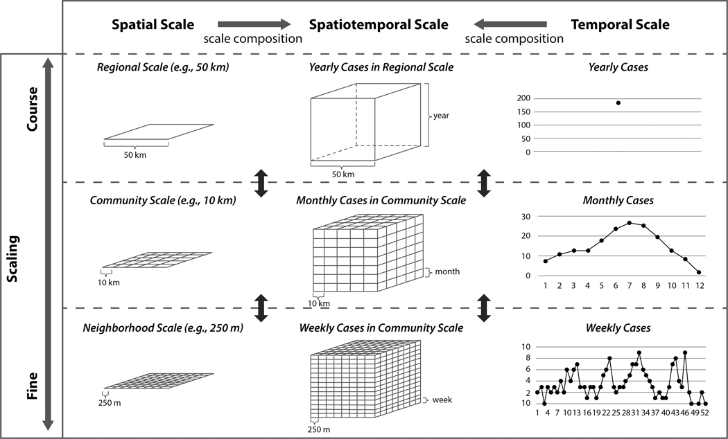
As discussed in the introduction, the aggregated statistics used in UA-GSA meet the inevitable issues associated with the zoning effects of MAUP and MTUP that are likely to impact the results of UA-GSA. ABMs of communicable diseases often produce point pattern data about outbreaks (i.e., longitude, latitude and timestamp) as outcomes. Such point-based measures are often aggregated at certain spatial and temporal scales. Figure 1 illustrates how model outputs can be summarized at multiple scales. Spatial patterns of disease outbreaks can be described as regional, community, or neighborhood scale patterns. Temporal patterns can be explained as yearly, monthly, or weekly cases. The output scales can be summarized as yearly cases at a regional scale, monthly cases at a community scale, or weekly cases at a neighborhood scale.
Figure 1.
Spatiotemporal scaling of model outputs
UA-GSA takes statistics (e.g., dengue infection rates or the number of dengue cases) from each simulation run. UA-GSA at a yearly regional scale may be performed once. Importantly, to carry out UA-GSA at multiple spatiotemporal scales, multiple executions of UA-GSA are required. Running UA-GSA multiple times may be computationally intensive. For example, suppose that we ran the simulation for 1 year within the study area (10 km × 10 km) and plan to perform the UA-GSA at finer scales (e.g., weekly patterns in neighborhood scales (250 m × 250 m)). The number of times that UA-GSA need to be performed is equal to 1,600 (40 × 40). If each UA-SA will take 1 minute and then, the total amount of time will be approximately 26.67 hours.
3. Methods
3.1. A spatially explicit ABM of dengue virus transmission
In this paper, we used a spatially explicit ABM of dengue transmission (Kang & Aldstadt, 2019b), which was implemented in Anylogic 7.3.5. For the details of this model, please see the Overview, Design Concepts and Details (ODD) protocol (Grimm et al., 2010) provided in Kang and Aldstadt (2019b). The model is also available at the Anylogic cloud (https://cloud.anylogic.com/model/64d09b7f-fcd6-4b04-af26-834a26be569d?mode=SETTINGS). In the model, there are three main components: (1) human agents, (2) mosquito agents, and (3) an environment. The ABM considers the nature of dengue transmission; there are four distinct serotypes of dengue, but they are serologically related to each other. An infection from one serotype of dengue provides a lifelong immunity to that serotype with cross-protection to other serotypes for 120 days (Chao et al., 2012). After 120 days, individuals again become susceptible to serotypes that they have not been previously infected with (Vaughn et al., 2000).
In this model, DENV epidemics occur through interactions between human and mosquito agents. Such interactions for the dengue transmission are described with a SEIR model (Susceptible-Exposed-Infectious-Recovered). Because there are four serotypes of dengue, each individual has four SEIR statuses. A susceptible individual is able to be exposed to dengue serotype that he/she has not been previously exposed to. An exposed individual who comes into contact with dengue through an infectious mosquito’s bite is not able to transmit the virus during the incubation period. An infectious individual can transmit the virus to susceptible mosquitoes. A recovered individual is no longer susceptible to that serotype of dengue.
To estimate an individual human’s dengue exposure prior to the dengue epidemic simulations, it is assumed that all individuals are exposed to dengue with an annual attack rate of 0.14, regardless of serotypes. The lack of consideration for serotypes related to prior exposure to dengue virus may be responsible for aspatial structures of community-level immunity (Kang & Aldstadt, 2019b). Given the seasonal serotype-specific dominance in Thailand (Nisalak et al., 2003) and the focality of dengue outbreaks (Mammen Jr et al., 2008), the immunity statuses of individuals should be similar to that of their neighbors. Therefore, we incorporated a burn-in period; dengue epidemic simulations were carried out for five years, but only the final year’s output was utilized in this study.
In this model, individual human agents have age-specific commuting behaviors, as shown in Figure 2 (A). First of all, people aged 5 to 19 and those aged 20 to 64 typically commute their schools and workplaces around 9am, respectively, and they come back home around 5pm. Second, everyone else stays at home. Those who become infected stay at their home until they are recovered (Kang & Aldstadt, 2019b).
Figure 2.
Agent’s movement. (A) human agent’s movement; (B) mosquito agent’s movement
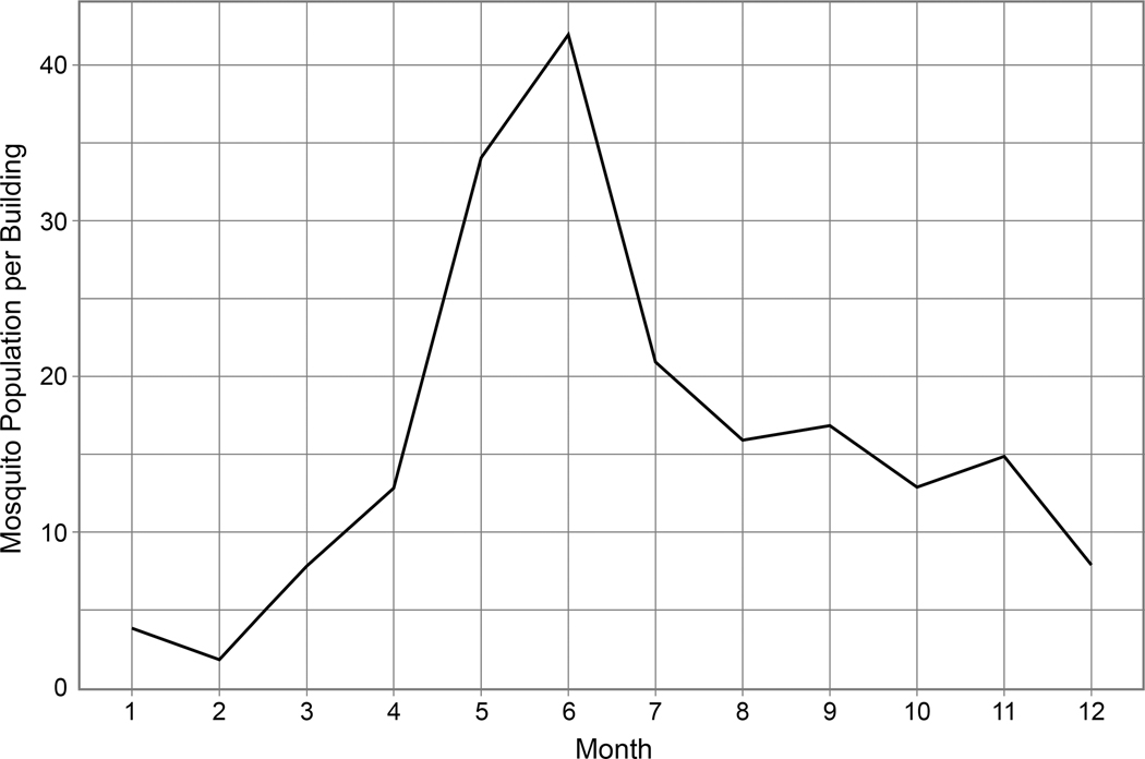
Mosquito agents refer only to infected female mosquitoes. The number of female mosquitoes per building represents mosquito breeding and feeding sites. If an infectious human is in range, one or more susceptible mosquitoes may bite the human. If it bites an infectious human it will become an agent. Once infected mosquitoes become infectious, they can transmit dengue to co-located susceptible human agents during their lifetime. The mosquitoes can also travel to neighboring houses (within 30 meters) with a 0.15 probability per day (Chao et al., 2012) (Figure 2 (B)). Because summer in Thailand is hot and humid, the initial number of mosquitoes is set to 42 in June (Chao et al., 2012) (Figure 3). We also assume that the maximum number of mosquitoes is the same in every building. The biting behavior for mosquitoes occurs at four discrete time intervals (08–13 h, 13–18 h, 18–24 h, and 00–08 h) with biting rates of 0.08, 0.76, 0.13, and 0.03, respectively. How long a mosquito agent survives depends on its age (Harrington et al., 2001; Harrington et al., 2008; Harrington et al., 2005).
Figure 3.
Seasonal mosquito population estimated per building
3.2. Study area and data
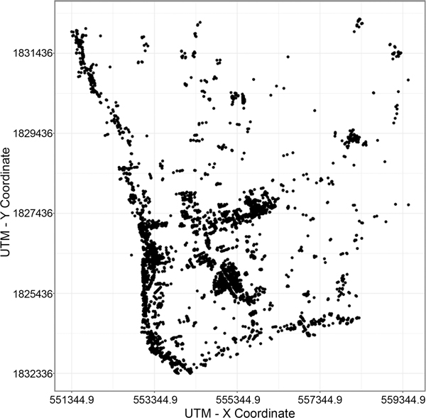
The study area lies in a portion of northeastern Kamphaeng Phet province in Thailand. In the area there are 3,683 households, 185 workplaces, and 8 schools. A LIDAR-derived building dataset was utilized to indicate the locations of all buildings in the study area (Figure 4). A household dataset collected in 2009 (Thomas et al., 2015) was used to assign the number of households and the ages of household members. Based on birth rates and death/out-migration rates calculated from population register data obtained from the Department of Provincial Administration, Ministry of Interior Thailand, the population was updated every year.
Figure 4.
Spatial distribution of households in the study area
3.3. CyberGIS-enabled spatiotemporally explicit UA-SA
3.3.1. Workflow
Monte Carlo (MC) simulations are required prior to performing UA-GSA. MC simulations are executed by varying the uncertain input parameters of interest, which are often chosen from quasi-random sampling (Saltelli, Tarantola, & Chan, 1999). We ran 16,000 simulations of the ABM of dengue virus transmission. The equation for calculating the number of simulation runs is provided in Section 3.3.2. Each simulation produces an output. In the case of dengue simulations, the simulation output consists of point pattern data about outbreaks (i.e., longitude, latitude and timestamp). The details of the MC simulations conducted in this paper are provided in Section 3.3.2.
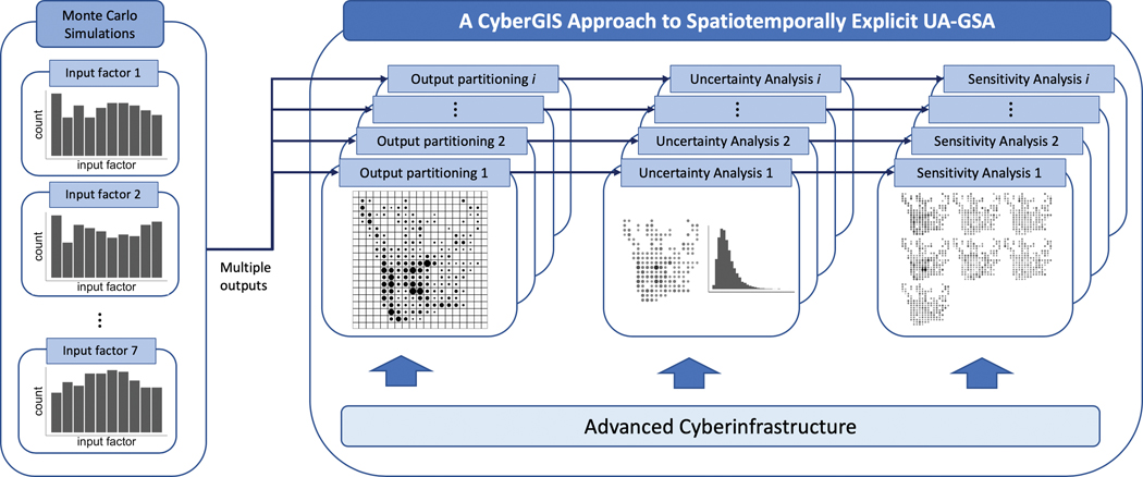
The workflow of a cyberGIS approach to spatiotemporally explicit UA-GSA is as follows: 1) determine sets of spacetime scales, 2) partition the model outputs at each spacetime scale, 3) measure the average and variance of the model outputs for the spatiotemporally explicit UA, and 4) measure the first-order sensitivity index and total sensitivity index for the spatiotemporally explicit SA (Figure 5). These tasks concerning partitioning, UA, and GSA should ideally be performed on advanced cyberinfrastructure, which provides high performance computing power to resolve the computational burdens of UA-GSA at multiple spatiotemporal scales.
Figure 5.
Workflow of cyberGIS-approach spatiotemporally explicit UA-GSA
In our study, UA-GSA was performed at multiple space-time scales (Table 1). Since the spatial extent of the study area is approximately 8,900 × 8,200 (meters), the coarsest spatial resolution is 9,000 × 9,000 (meters). Additionally, we used simulated outcomes for the final year after a burn-in period of four years. The coarsest temporal extent is one year. Here, the temporal scale refers to time span instead of timestamp. For example, infection rates for 6 months denote the average over seven monthly infection rates (Jan to Jun, Feb to Jul, Mar to Aug, Apr to Sep, May to Oct, Jun to Nov, and Jul to Dec). Our research focuses on investigating the impact of input factors on not just events of dengue transmission, but also on a series of processes of dengue transmission. Therefore, it is more suitable to consider time span as a temporal scale. Each UA-GSA is performed at jointly combined spatiotemporal scales. Given eight spatial scales and ten temporal scales, as provided in Table 1, we perform 80 times of UA-GSA. For example, UA-GSA is performed at 9000 × 9000 spatial scale with one-year temporal scale, and then, it is performed at 9000 × 9000 spatial scale with six months temporal scale. This way of UA-GSA would help to gain an improved understanding about spatiotemporal scaling effects of parameters on their uncertainty and sensitivity in spatially explicit agent-based modeling.
Table 1.
Spatiotemporal extents
| Scales | Units |
|---|---|
| Spatial Scales | 9000 × 9000, 5000 × 5000, 3000 × 3000, 1000 × 1000, 500 × 500, 300 × 300, 100 ×100, 50 × 50 (meters) |
| Temporal Scales | 1 year, 6 months, 3 months, 2 months, 1 month, 2 weeks, 1week, 3 days, 2 days, 1 day |
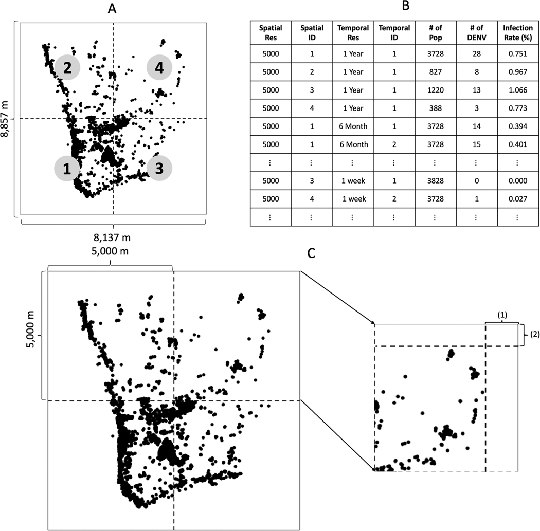
To perform UA-GSA at multiple spatiotemporal scales, we need to summarize the simulated dengue outbreaks at each spatiotemporal scale provided in Table 1. Figure 6 shows an example after pre-processing spatiotemporally explicit UA-GSA within 3000-meter spatial grids. The outputs from simulations are summarized at each spatiotemporal grid, as shown in Figure 6 (A) and (B). The table includes spatial resolution, a spatial ID representing the relative location where each grid is positioned, temporal resolution, a temporal ID representing the time span, human population, the number of dengue cases, and the infection rates. Because our study area is not squarely shaped, we created margins of appropriate size on the width (1) and height (2) (Figure 6 (C)). In Figure 6 (C), width (1) is equal to 931.5 (= (10,000 – 8,137) / 2) meters and height (2) is 571.5 (= (10,000 – 8,857) /2) meters, respectively.
Figure 6.
Pre-processing. (A) spatial extents; (B) summary table; (C) spatial margins
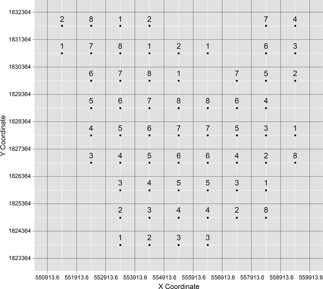
The UA-GSA was performed in parallel. Figure 7 illustrates an example of parallel processes of the spatiotemporally explicit UA-GSA within 1000-meter spatial grids. Although the study area was decomposed into 81 grids, households exist within only 60 grids. Therefore, 60 grids will be run on eight processors.
Figure 7.
An example of a parallel process of spatiotemporally explicit UA-GSA within 1,000-meter spatial grids. The numbers above dots denote which processors will perform UA-GSA.
As there are four remainders, four separate processors are also assigned with the additional runs. In other words, four processors will run the UA-GSA seven times, and four processors will run eight times. This parallelization applies to the UA-GSA at varying spatial grids (i.e., 9000 × 9000, 5000 × 5000, 3000 × 3000, 1000 × 1000, 500 × 500, 300 × 300, 100 ×100, 50 × 50). Each run contains the UA-SA at varying time spans (i.e., 1 year, 6 months, 3 months, 2 months, 1 month, 2 weeks, 1 week, 3 days, 2days, and 1 day).
To run the simulation, we employed Virtual ROGER (a cyberGIS supercomputer hosted by the CyberGIS Center for Advanced Digital and Spatial Studies at University of Illinois at Urbana-Champaign). In this study, we did not need to fully make use of cutting-edge high-end technology for computation. Harnessing the accessible high-performance computing power with GPU nodes and memory enables us to perform the spatiotemporally explicit UA-GSA in a computationally efficient manner. The ability to utilize these resources with minimal effort underscores how easily accessible processing resources can be.
Our cyberGIS approach to uncertainty and global sensitivity analysis for spatially explicit agent-based modeling shows how the use of advance cyberinfrastructure could help to carry out uncertainty and sensitivity analysis at multiple spatiotemporal scales. This approach allows one to examine the uncertainty and sensitivity of parameters at simultaneously finer and coarser spatiotemporal scales. In fact, our analysis is successively performed varying spatial grids and time spans. Therefore, this approach conceptually contributes to expanding the usefulness of CyberGIS and cyberinfrastructure in uncertainty and sensitivity analysis for agent-based modeling.
3.3.2. UA-GSA
In the case of the dengue virus transmission model, the model output is spatiotemporal point patterns of dengue cases. The output could be aggregated to derive school population infection rates (Endy et al., 2002) or community-level cluster investigations as reported by Yoon et al. (2012). Due to the uncertainty in model inputs and the stochastic nature of ABMs (Rahmandad & Sterman, 2008), there is output variability. The uncertainty in model inputs may also be responsible for difficulties in understanding relationships between model inputs and outputs.
For addressing this issue, UA-GSA helps to quantitatively assess the variation in the model outputs and the contributions of model inputs to the variation (Crosetto & Tarantola, 2001; Hu et al., 2017). UA examines uncertainty in model outputs, which are attributed to model inputs. As a result, UA demonstrates the variability in model outputs. On the other hand, GSA investigates how the variability in model outputs depend on the model inputs (Saltelli et al., 1999). In the literature, SA is categorized into local and global approaches. A local SA approach is also called one-at-a-time (OAT). By varying a parameter within ± 10 – 20 %, a local SA examines how such input variation contributes to changes in model outputs. However, a local SA approach is not able to quantify the effects of interactions between multiple input factors on model outputs (Crosetto, Tarantola, & Saltelli, 2000). For example, in communicable disease models, infections require at least collocations of infectious and susceptible humans, which are specified by parameters related to agent state transitions (i.e., incubation period; duration after which a human become infectious) and interactions between agents (i.e., contract rate; the effectiveness of contact for infection transmission) (Mao & Bian, 2010). In addition, the model outcomes in ecological models, such as egg productions, are also related to agent state transition (i.e., life-stage; egg, yolk-sac larvae, larvae, juvenile or adult) and the interactions between agents and their environment (i.e., temperature) (Boyd, Roy, Sibly, Thorpe, & Hyder, 2018). To account for these factors, another type of SA needs to be performed.
Variance-based GSA is well suited to ABMs that are inherently associated with nonlinearity. GSA helps to decompose the variance in model outputs into first-order effects and higher order effects resulting from interactions between input factors (Saltelli et al., 1999). The results from GSA provide the magnitude of impacts of input factors on the variability of model outputs. A GSA can be described using the following equation:
where V denotes the variance in model outputs, Vi stands for the first order effects of V due to input parameter i. Vij represents the second order effects of V due to the interaction between input factor i and j. Vijk denotes the third order effects of V contributed by the interactions among input factor i, j, and k. V12…m denotes the highest order effects of V explained by the interactions between all input factors used in GSA. m represents the number of input factors.
A first order sensitivity index (Si) explains the decoupled effects of a single input factor on variance in model outputs. Based on the decomposition of variance, the first-order sensitivity index can be derived in the following way:
The first-order sensitivity index for a given input factor ranges from zero to one, and the sum of the first-order indexes of all input factors are less than or equal to one. If the sum of the first-order indexes equals one, it means there are no interaction effects among input parameters. On the other hand, if the sum of the first-order indexes is less than one, interaction effects are present. Therefore, the effects of interaction among input factors are derived as follows:
The total sensitivity index (STi) describes the effects of a given input factor (i) to V, and is composed of both a single effect of the factor and its interaction effects with other input factors. The total sensitivity index is derived based on the following equation:
where Si is first-order sensitivity index of factor i. Sij is second-order sensitivity index of the interaction effects between i and j. Sijk is third-order sensitivity index of the interaction effect among i, j, and k.
In this paper, spatiotemporally explicit UA-GSA comprises examining the uncertainty in the environment, the interactions between agents, agents’ behaviors, and agent state transitions. In this model, the parameter explicitly referring to the interactions between agents and the environments does not exist. Seven parameters are drawn from a uniform distribution within 50% variation from a baseline value (Table 2). We conducted 16,000 model experiments using a Monte Carlo approach, using the following settings: Introduction Rates (IR) U ~ [1.0e−6, 1.0e−5], Probability of Infection from Mosquito to Person (PMP) U ~ [0.125, 0.375], Probability of Infection from Person to Mosquito (PPM) U ~ [0.05, 0.15], Daily Movement Probability of Mosquito (MR) U ~ [0.075, 0.225], Movement Distance of Mosquito (MD) U ~ [15, 45], Extrinsic Incubation Period of Mosquito (EIP) U ~ [5.5, 16.5], and Incubation Period of Human (IP) U ~ [3, 9].
Table 2.
The ranges of input parameters used in Monte Carlo simulations
| Parameters | Descriptions (Units) | Lower | Baseline | Upper | |
|---|---|---|---|---|---|
| Environment | IR | Introduction rate of dengue outside study area (person per person) | 1.5e−6 (−50%) | 1.0e−5 | 1.5e−5 (+50%) |
| Agent Interaction | PMP | Probability of infection from mosquito to person (case per case) | 0.125 (−50%) | 0.25 | 0.375 (+50%) |
| PPM | Probability of infection from person to mosquito (case per case) | 0.05 (−50%) | 0.1 | 0.15 (+50%) | |
| Agent Behavior | MR | Daily movement rate of mosquito (1/day) | 0.075 (−50%) | 0.15 | 0.225 (+50%) |
| MD | Movement distance radius of mosquito (meter) | 15 (−50%) | 30 | 45 (+50%) | |
| Agent State Transition | EIP | Extrinsic incubation period of mosquito (day) | 5.5 (−50%) | 11 | 16.5 (+50%) |
| IP | Incubation period (day) | 3 (−50%) | 6 | 9 (+50%) | |
The total number of simulation runs are derived from Tang and Jia (2014), as follows:
where is the number of input factors used in GSA and is the number of Monte Carlo runs associated with the sampling. It is suggested that be set within the range of [20, 100] (Tang & Jia, 2014). In this paper, we ran 1,000 Monte Carlo runs to create sufficient samples of each input factor used in UA-GSA. Therefore, with seven input factors, the total number of simulation runs is 16,000.
4. Results
4.1. Spatiotemporally explicit UA
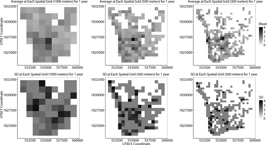
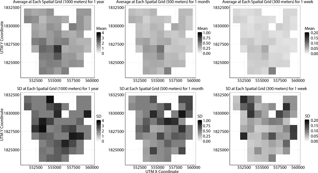
Spatiotemporally explicit UA illustrates how the mean and standard deviation (SD) of infection rates vary depending on spatiotemporal scales. As examples, Figures 8 and 9 show that uncertainty in infection rates depends on varying spatial or temporal scales. In these examples, the points represent the centroids of spatial grids. When it comes to uncertainty in infection rates by varying spatial scales, the average of infection rates at each spatial grid does not look dramatically change at each spatial grid, but there are apparent changes in standard deviation (Figure 8). As the spatial scale becomes finer, the SD at each grid becomes larger (Figure 9). The variability between simulations is generally larger when geographic areas and correspondingly populations at risk are smaller.
Figure 8.
Uncertainty variation across spatial scales
Figure 9.
Uncertainty variation across temporal scales
With varying temporal scales, large changes in the averages and SD of infection rates appear. Overall, both averages and SD become smaller as the temporal scales become smaller. Both Figures 8 and 9 show scale-dependent uncertainty. To understand which input factors may be responsible for such scale-dependent uncertainty in infection rates, spatially explicit GSA should be performed.
4.2. Spatiotemporally explicit GSA
The results from the spatiotemporally explicit GSA provide a better understanding of the associations between model inputs and outputs. Particularly, our GSA helps in identifying influential factors related to the variability of infection rates at each spatiotemporal scale. The GSA results in Si and TSi. S explains the effect of a given factor on variance of infection rates at a particular spacetime scale. TS represents the impact of a given factor and its interactions with other factors on variance of infection rates at a particular spacetime scale. Following Ligmann-Zielinska and Sun (2010), S and TS can be interpreted as follows: 1) a relatively higher S indicates that the impact of a given factor on variability of infection rates is relatively greater than other factors, and 2) a relatively higher TS means that the impact of a given factor involved in interactions with other input factors on the variability of infection rates is relatively greater than other factors.
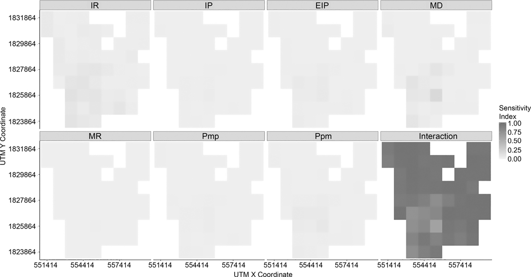
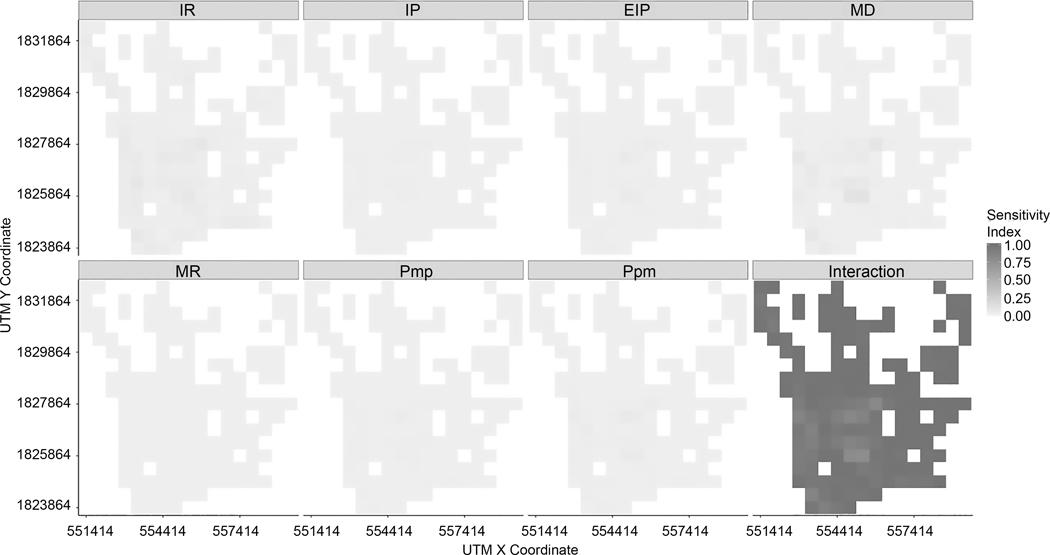
Based on first-order sensitivity indices, we found that the interaction between all factors was the most influential to the variance in infection rates. While single factor impacts decrease, the effect of between-factor interactions on the variability of infection rates increases. As shown in Figure 10, within 1000-meter grids, all seven input factors have weaker impacts on variability in model outputs, which means 1–34 % of the variability can explain the variance in infection rates at each grid cell. In other words, about 66 – 99% of the variability is attributed to interaction among seven factors (i.e., IR, PMP, PPM, IP, EIP, MD, and MR). In addition, within 500-meter grids (Figure 11), only about 0–21 % of variability can be explained by input factors taken singly. The interaction of all seven input factors can explain approximately 78–100% of variability.
Figure 10.
First-order indices of input factors at 1000-meter grid for a 1-year time span
Figure 11.
First-order indices of input factors at 500-meter grid for 1-year time span
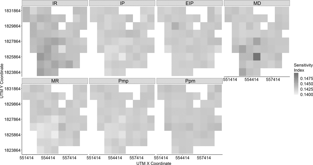
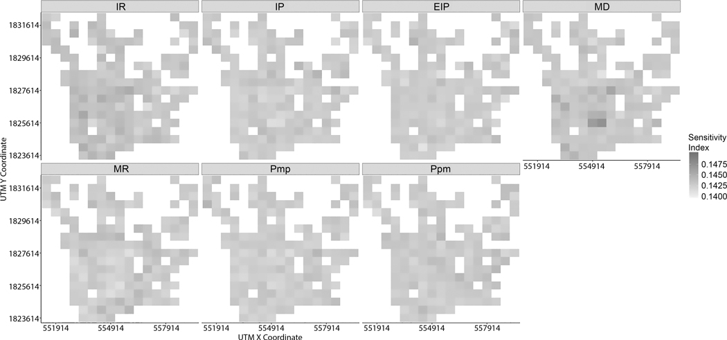
Because individual factors (first-order sensitivity indices) cannot directly explain the variability in infection rates, total effect sensitivity indices need to be used to account for the variance in model outputs. The normalized TS describes both the impact of a given factor and its interactions with other factors. Spatial patterns of the normalized TS of each factor look to be spatially randomly distributed (Figures 12 and 13). There seems to be no particularly general patterns in the normalized TS. However, it is shown that each input factor has spatially varying effects on outcomes at different spatial locations (Figures 12 and 13).
Figure 12.
Total sensitivity indices of input factors within a 1000-meter grid for 1-year time span
Figure 13.
Total sensitivity indices of input factors at a 500-meter grid for a 1-year time span
Particularly, TS of mosquito movement distance (MD) is related to household density (Figure 14 (A)). The spatial patterns of TS for MD look similar to the spatial configuration of household density (Figure 14 (B)). Spearman’s rank correlation coefficient was used due to the right-skewed distribution of household density. Spearman’s correlation coefficient between household counts and TS of MD is equal to 0.56 (p <0.001). As Kang and Aldstadt (2017) highlight, the spatiotemporal patterns of dengue outbreaks are likely to be related to the spatial configurations of buildings in which mosquitoes can reside in and travel between. Therefore, a higher household density results in more possible mosquito destinations, which in turn may lead to more dengue infections in nearby households. In addition, TS of introduction rates (IR) is also moderately related to household density (Figure 14 (C)). Spearman’s’ correlation coefficient between household counts and TS of IR is equal to 0.352 (p<0.001). When pathogens are introduced to a dense area, dengue may be increasingly transmitted within the region since there are more human hosts. Although all regions do not have significant relationships between the household density and TS of MD and TS of IR, some regions at higher household density (highlighted with red-circle in the Figure 14) show relatively higher impacts of MD and IR.
Figure 14.
Relationship between TS of MD and IR, and household density: (A) household density within 500-meter spatial grids, (B) TS of MD within 500-meter spatial grids, and (C) TS of IR within 500-meter spatial grids. The red circles represent the regions at higher household density.
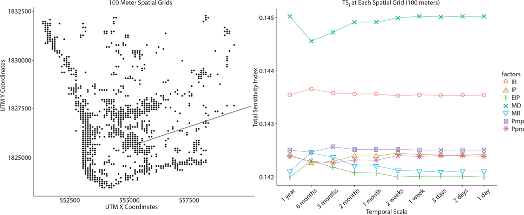
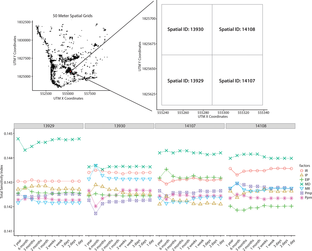
Greater impacts of MD were also found at very fine spatial scales (i.e., 100-meter spatial grids and 50-meter spatial grids). Figure 15 illustrates TS at the spatial grid cell in which households were the most spatially clustered within 100-meters. Figure 15 shows TS at sub-spatial grids of the spatial grid shown in Figure 16. At a 100-meter scale, MD was the most influential to infection rates, and IR was moderately influential. Compared to these two factors, MD and IR, the other five factors relatively have a weaker effect on the variability of infection rates in each spatial grid.
Figure 15.
TS within a finer spatial grid (100 meters)
Figure 16.
TS within a finer spatial grid (50 meters). The number on the top of the lower figure denotes the spatial ID.
Interestingly, although MD has the greatest effect on outcomes at a 100-meter scale, the effect at 50-meter sub-grids (spatial ID 13930, 14107, and 14108) was not as great as that at a 100-meter scale. Instead, it is shown that MR and EIP greatly affect model outputs at the finer resolution. This result is consistent with the often-observed clustering of household-level dengue infections. For example, Yoon et al. (2012) found spatially clustered patterns of infections; 35% of household members of infected children were also infected in the same time period, which means these focal successive dengue infections are not influenced by mosquito movement distances. Therefore, mosquito movement distances had relatively less impact on dengue outbreaks in the 50m cells. When the pathogen is introduced into these small areas, MR and EIP are more important in determining the intensity of successive infections in the same household.
The magnitude of TS varies depending on temporal scale. In general, the magnitudes are similar to those of 1 year, 2 weeks, 1 week, 3 days, 2 days, and 1 day, while those of 6 months, 3 months, and 2 months are different from the rest. This pattern may be related to seasonality in dengue epidemics and the time period of successive transmission of dengue virus (two to three weeks (Aldstadt, 2007)). Due to seasonality in mosquito density (Figure 3), dengue outbreaks frequently occur during summer, such as for 4 months (April to July) or 6 months (April to September). Given that we used the averages of infection rates as a statistic in UA-GSA, these time spans may contribute to such different TS results at some temporal scales (6 months, 3 months, 2 months and 1 month).
5. Conclusion
Although much effort on UA-GSA have been made to understand uncertainty in ABM results arising from model inputs, the research question about how the impacts of modeling inputs on the variability in modeling outputs vary at each space-time scale remains to be solved. In this study, we attempted to answer the research question by measuring the scale-specific effects (spatial, temporal and spatiotemporal) on modeling outputs. Our case study used a spatially explicit ABM of dengue virus transmission from Kang and Aldstadt (2019b). We performed variance-based GSA to measure the contributions of input factors to infection rates at various spatiotemporal scales. The input factors that were tested include introduction rates, the probability of transmission from mosquito to human, the probability of transmission from human to mosquito, the human incubation period, the extrinsic human incubation period, mosquito movement distance, and mosquito movement rates.
The results from the UA-GSA particularly show that input factors have scale-varying impacts on variability in model outputs. In other words, input factors may have relatively large impacts in certain regions, but there may not be significant effects at other regions. Such spatial effects also vary between temporal scales. Sensitivity indices are correlated with the spatial configurations of places that govern where agents can reside and travel to. For example, the sensitivity of parameters about agent movement (i.e., MD) are strongly influenced by spatial scales. The cyberGIS approach has the primary benefit of reducing the runtime for UA-SA, showing promise for enabling computationally intensive spatiotemporal analytics.
A cyberGIS approach to spatiotemporally explicit UA-GSA provides an improved understanding of the associations between model inputs and outputs at a range of spatiotemporal scales. By performing UA-GSA in parallel manner leveraging high-performance computing power, provided by advanced cyberinfrastructure we were able to cope with computational intensity that is still challenging for personal computing. The multiple spatiotemporal scales of UA-GSA also well reflect the POM paradigm (Grimm & Railsback, 2012; Grimm et al., 2005) that has already been advocated for evaluating and validating spatially explicit ABMs. The POM paradigm could serve as a guide for initializing models (Fedriani et al., 2018; Liukkonen et al., 2018). Following the POM, the patterns of modeling outputs can also be used as an indicator for validating a model’s underlying assumptions (Kang & Aldstadt, 2019b) and evaluating parameters (Kang & Aldstadt, 2019a). This study advances the usefulness space-time patterns to measure the effects of a model’s parameters on modeling outputs from local to global scales.
Importantly, based on the results from performing GSA at very fine spatial scales, we found that the proper spatiotemporal scale may need to be selected based on the research questions being addressed. Given that ABMs are often used to examine various scenarios by varying input parameters, the way that UA-GSA are presented in this paper would be helpful for investigating the effectiveness of particular policies at multiple space-time scales. In detail, the relatively greater effects of mosquito movement at regions in which households are highly clustered underscore the potential utility of mosquito removal to control dengue virus transmission, as highlighted by previous studies (Achee et al., 2015; Scott & Morrison, 2010). In addition, the greater sensitivity in mosquito movement distance also indicates the importance of proper parameterization of agent movement. Where greater effects of introduction rates are found, proper levels of surveillance for people who travel outside the community needs to be considered for better prevention and control of dengue outbreaks. Our spatiotemporally explicit UA-GSA may also help in investigating the effects of input factors on model outcomes that are particularly spatially and temporally clustered, such as violence and communicable disease transmission.
Given that the usefulness of variance-based GSA in implementing parsimonious ABMs (Ligmann-Zielinska, 2018; Ligmann-Zielinska et al., 2014), simplification of the ABMs would be an apparent next step. The parsimonious ABMs of dengue virus transmission within advanced cyberinfrastructure may help to explore the dynamic nature of dengue virus transmission in a computationally efficient way. The investigation on the non-quantifiable uncertainty of the modeling parameters at an initial stage of modeling would be also one of the future directions. In this paper, we only used infection rates at each spatiotemporal scale. Given that various spatio-temporal statistics, such as the Knox Test (Knox, 1964), the incremental Knox test (Aldstadt, 2007), and the Getis-Ord GI* statistic (Getis & Ord, 1992) are useful for detecting spatially and temporally clustered dengue patterns, it would be interesting to use such indicators as a statistic in UA-GSA. The results would assess how such input factors impact not only simple aggregate measures (i.e., dengue infection rates), but also the spatiotemporal clustering of simulated patterns. A cyberGIS approach would also help to resolve a computational intensity that may be faced with carrying out such spatio-temporal statistics for analyzing modeling outputs.
Acknowledgements
The authors would like to express appreciation for the funding provided by the National Institutes of Health (R01 GM083224 and P01 AI034533) and the National Science Foundation (1743184 and 1443080). Our computational work used Virtual ROGER, which is a cyberGIS supercomputer supported by the CyberGIS center for Advanced Digital and Spatial Studies and the School of Earth, Society and Environment at the University of Illinois at Urbana-Champaign.
Biography
Jeon-Young Kang
JEON-YOUNG KANG is a postdoctoral research associate at the CyberGIS Center for Advanced Digital and Spatial Studies at the University of Illinois at Urbana-Champaign, Urbana, IL, 61801. geokang@illinois.edu. His research interests focus on geographic information science, agent-based modeling, cyberinfrastructure, and health geography.
Jared Aldstadt
JARED ALDSTDT is an associate professor of Geography at the State University of New York at Buffalo, Buffalo, NY, 14261. geojared@buffalo.edu. He is a medical geographer and spatial modeler specializing in the ecology of infectious disease, including mosquito-borne pathogens.
Rebecca Vandewalle
REBECCA VANDWALLE is a Ph.D. student in the Department of Geography and Geographic Information Science at the University of Illinois at Urbana-Champaign, Urbana, IL, 61801. rcv3@illinois.edu. Her research interests are geographic information science, high-performance computing, cyberinfrastructure, and natural hazards.
Dandong Yin
DANDONG YIN is a Ph.D. candidate in the in the Department of Geography and Geographic Information Science at the University of Illinois at Urbana-Champaign, Urbana, IL, 61801. dyin4@illinois.edu. His research interests are geographic information science, high-performance computing, cyberinfrastructure, and natural hazards.
Shaowen Wang
SHAOWEN WANG is a professor and head of the Department of Geography and Geographic Information Science at the University of Illinois at Urban-Champaign, Urbana, IL, 61801. shaowen@illinois.edu. His research interests focus on geographic information science and systems (GIS), advanced cyberinfrastructure and cyberGIS, complex environmental and geospatial problems, computational and data sciences, high-performance and distributed computing, and spatial analysis and modeling.
References
- Achee N, Gould F, Perkins TA, Reiner R Jr, Morrison A, Ritchie S, … Scott T. (2015). A critical assessment of vector control for dengue prevention. PLoS neglected tropical diseases, 9(5), e0003655. [DOI] [PMC free article] [PubMed] [Google Scholar]
- Aldstadt J. (2007). An incremental Knox test for the determination of the serial interval between successive cases of an infectious disease. Stochastic Environmental Research and Risk Assessment, 21(5), 487–500. [Google Scholar]
- An L, Linderman M, Qi J, Shortridge A, & Liu J. (2005). Exploring Complexity in a Human–Environment System: An Agent-Based Spatial Model for Multidisciplinary and Multiscale Integration. Annals of the Association of American Geographers, 95(1), 54–79. [Google Scholar]
- Bitterman P, & Bennett DA (2016). Constructing stability landscapes to identify alternative states in coupled social-ecological agent-based models. Ecology and society, 21(3). [Google Scholar]
- Boyd R, Roy S, Sibly R, Thorpe R, & Hyder K. (2018). A general approach to incorporating spatial and temporal variation in individual-based models of fish populations with application to Atlantic mackerel. Ecological Modelling, 382, 9–17. [Google Scholar]
- Chao D, Halstead S, Halloran ME, & Longini I Jr (2012). Controlling dengue with vaccines in Thailand. PLoS Neglected Tropical Diseases, 6(10), e1876. [DOI] [PMC free article] [PubMed] [Google Scholar]
- Crooks A, Castle C, & Batty M. (2008). Key challenges in agent-based modelling for geospatial simulation. Computers, Environment and Urban Systems, 32(6), 417–430. [Google Scholar]
- Crooks A, & Hailegiorgis A. (2014). An agent-based modeling approach applied to the spread of cholera. Environmental Modelling & Software, 62, 164–177. [Google Scholar]
- Crosetto M, & Tarantola S. (2001). Uncertainty and sensitivity analysis: tools for GIS-based model implementation. International Journal of Geographical Information Science, 15(5), 415–437. [Google Scholar]
- Crosetto M, Tarantola S, & Saltelli A. (2000). Sensitivity and uncertainty analysis in spatial modelling based on GIS. Agriculture, ecosystems & environment, 81(1), 71–79. [Google Scholar]
- Endy TP, Chunsuttiwat S, Nisalak A, Libraty DH, Green S, Rothman AL, … Ennis FA (2002). Epidemiology of inapparent and symptomatic acute dengue virus infection: a prospective study of primary school children in Kamphaeng Phet, Thailand. American Journal of Epidemiology, 156(1), 40–51. [DOI] [PubMed] [Google Scholar]
- Fedriani JM, Wiegand T, Ayllón D, Palomares F, Suárez-Esteban A, & Grimm V. (2018). Assisting seed dispersers to restore oldfields: An individual-based model of the interactions among badgers, foxes and Iberian pear trees. Journal of applied ecology, 55(2), 600–611. [Google Scholar]
- Getis A, & Ord JK (1992). The analysis of spatial association by use of distance statistics. Geographical analysis, 24(3), 189–206. [Google Scholar]
- Grant TJ, Parry HR, Zalucki MP, & Bradbury SP (2018). Predicting monarch butterfly (Danaus plexippus) movement and egg-laying with a spatially-explicit agent-based model: The role of monarch perceptual range and spatial memory. Ecological Modelling, 374, 37–50. [Google Scholar]
- Grimm V, Berger U, DeAngelis DL, Polhill JG, Giske J, & Railsback SF (2010). The ODD protocol: a review and first update. Ecological modelling, 221(23), 2760–2768. [Google Scholar]
- Grimm V, & Railsback SF (2012). Pattern-oriented modelling: a ‘multi-scope’for predictive systems ecology. Philosophical Transations of the Royal Society B, 367(1586), 298–310. [DOI] [PMC free article] [PubMed] [Google Scholar]
- Grimm V, Revilla E, Berger U, Jeltsch F, Mooij WM, Railsback SF, … DeAngelis DL (2005). Pattern-oriented modeling of agent-based complex systems: lessons from ecology. Science, 310(5750), 987–991. [DOI] [PubMed] [Google Scholar]
- Harrington LC, Buonaccorsi JP, Edman JD, Costero A, Kittayapong P, Clark GG, & Scott TW (2001). Analysis of survival of young and old Aedes aegypti (Diptera: Culicidae) from Puerto Rico and Thailand. Journal of Medical Entomology, 38(4), 537–547. [DOI] [PubMed] [Google Scholar]
- Harrington LC, Jones JJ, Kitthawee S, Sithiprasasna R, Edman JD, & Scott TW (2008). Age-dependent survival of the dengue vector Aedes aegypti (Diptera: Culicidae) demonstrated by simultaneous release–recapture of different age cohorts. Journal of Medical Entomology, 45(2), 307–313. [DOI] [PubMed] [Google Scholar]
- Harrington LC, Scott TW, Lerdthusnee K, Coleman RC, Costero A, Clark GG, … Sithiprasasna R. (2005). Dispersal of the dengue vector Aedes aegypti within and between rural communities. The American Journal of Tropical Medicine and Hygiene, 72(2), 209–220. [PubMed] [Google Scholar]
- Hu H, Lin T, Wang S, & Rodriguez LF (2017). A cyberGIS approach to uncertainty and sensitivity analysis in biomass supply chain optimization. Applied energy, 203, 26–40. [Google Scholar]
- Kang J-Y, & Aldstadt J. (2017). The Influence of Spatial Configuration of Residential Area and Vector Populations on Dengue Incidence Patterns in an Individual-Level Transmission Model. International Journal of Environmental Research and Public Health, 14(7), 792. [DOI] [PMC free article] [PubMed] [Google Scholar]
- Kang J-Y, & Aldstadt J. (2019a). Using multiple scale space-time patterns in variance-based global sensitivity analysis for spatially explicit agent-based models. Computers, Environment, and Urban Systems, 75, 170–183. [DOI] [PMC free article] [PubMed] [Google Scholar]
- Kang J-Y, & Aldstadt J. (2019b). Using multiple scale spatio-temporal patterns for validating spatially explicit agent-based models. International Journal of Geographical Information Science, 33(1), 193–213. [DOI] [PMC free article] [PubMed] [Google Scholar]
- Kang J-Y, & Aldstadt J. (2019c). Examining time-dependent effects of water, sanitation, and hygiene (WASH) interventions using an agent-based model. Tropical medicine & international health. 10.1111/tmi.13280 [DOI] [PubMed] [Google Scholar]
- Kim I-H, Tsou M-H, & Feng C-C (2015). Design and implementation strategy of a parallel agent-based Schelling model. Computers, Environment and Urban Systems, 49, 30–41. [Google Scholar]
- Knox E. (1964). The detection of space-time interactions. Applied Statistics, 13, 25–29. [Google Scholar]
- Ligmann-Zielinska A. (2013). Spatially-explicit sensitivity analysis of an agent-based model of land use change. International Journal of Geographical Information Science, 27(9), 1764–1781. [Google Scholar]
- Ligmann-Zielinska A. (2018). ‘Can You Fix It?’Using Variance-Based Sensitivity Analysis to Reduce the Input Space of an Agent-Based Model of Land Use Change GeoComputational Analysis and Modeling of Regional Systems (pp. 77–99): Springer. [Google Scholar]
- Ligmann-Zielinska A, Kramer DB, Cheruvelil KS, & Soranno PA (2014). Using uncertainty and sensitivity analyses in socioecological agent-based models to improve their analytical performance and policy relevance. PLoS One, 9(10), e109779. [DOI] [PMC free article] [PubMed] [Google Scholar]
- Ligmann-Zielinska A, & Sun L. (2010). Applying time-dependent variance-based global sensitivity analysis to represent the dynamics of an agent-based model of land use change. International Journal of Geographical Information Science, 24(12), 1829–1850. [Google Scholar]
- Liukkonen L, Ayllón D, Kunnasranta M, Niemi M, Nabe-Nielsen J, Grimm V, & Nyman A-M (2018). Modelling movements of Saimaa ringed seals using an individual-based approach. Ecological Modelling, 368, 321–335. [Google Scholar]
- Mammen MP Jr, Pimgate C, Koenraadt CJ, Rothman AL, Aldstadt J, Nisalak A, … Ypil-Butac CA (2008). Spatial and temporal clustering of dengue virus transmission in Thai villages. PLoS Medicine, 5(11), e205. [DOI] [PMC free article] [PubMed] [Google Scholar]
- Manson SM (2005). Agent-based modeling and genetic programming for modeling land change in the Southern Yucatan Peninsular Region of Mexico. Agriculture, ecosystems & environment, 111(1), 47–62. [Google Scholar]
- Mao L. (2011). Agent-based simulation for weekend-extension strategies to mitigate influenza outbreaks. BMC public health, 11(1), 522. [DOI] [PMC free article] [PubMed] [Google Scholar]
- Mao L, & Bian L. (2010). Spatial–temporal transmission of influenza and its health risks in an urbanized area. Computers, Environment and Urban Systems, 34(3), 204–215. [DOI] [PMC free article] [PubMed] [Google Scholar]
- Nisalak A, Endy TP, Nimmannitya S, Kalayanarooj S, Scott RM, Burke DS, … Vaughn DW (2003). Serotype-specific dengue virus circulation and dengue disease in Bangkok, Thailand from 1973 to 1999. The American Journal of Tropical Medicine and Hygiene, 68(2), 191–202. [PubMed] [Google Scholar]
- Openshaw S. (1984). The modifiable areal unit problem. [Google Scholar]
- Rahmandad H, & Sterman J. (2008). Heterogeneity and network structure in the dynamics of diffusion: Comparing agent-based and differential equation models. Management Science, 54(5), 998–1014. [Google Scholar]
- Saltelli A, Tarantola S, & Chan K-S (1999). A quantitative model-independent method for global sensitivity analysis of model output. Technometrics, 41(1), 39–56. [Google Scholar]
- Scott TW, & Morrison AC (2010). Vector dynamics and transmission of dengue virus: implications for dengue surveillance and prevention strategies. In Rothman A. (Ed.), Dengue virus (pp. 115–128). Berlin, Heidelberg: Springer. [DOI] [PubMed] [Google Scholar]
- Shook E, & Wang S. (2015). Investigating the Influence of Spatial and Temporal Granularities on Agent-Based Modeling. Geographical Analysis, 47(4), 321–348. [Google Scholar]
- Tang W, & Jia M. (2014). Global sensitivity analysis of a large agent-based model of spatial opinion exchange: A heterogeneous multi-GPU acceleration approach. Annals of the Association of American Geographers, 104(3), 485–509. [Google Scholar]
- Tang W, Wang S, Bennett DA, & Liu Y. (2011). Agent-based modeling within a cyberinfrastructure environment: a service-oriented computing approach. International Journal of Geographical Information Science, 25(9), 1323–1346. [Google Scholar]
- Thomas SJ, Aldstadt J, Jarman RG, Buddhari D, Yoon I-K, Richardson JH, … Rothman AL (2015). Improving dengue virus capture rates in humans and vectors in Kamphaeng Phet Province, Thailand, using an enhanced spatiotemporal surveillance strategy. The American Journal of Tropical Medicine and Hygiene, 93(1), 24–32. [DOI] [PMC free article] [PubMed] [Google Scholar]
- Vaughn DW, Green S, Kalayanarooj S, Innis BL, Nimmannitya S, Suntayakorn S, … Ennis FA (2000). Dengue viremia titer, antibody response pattern, and virus serotype correlate with disease severity. The Journal of Infectious Diseases, 181(1), 2–9. [DOI] [PubMed] [Google Scholar]
- Wang S. (2010). A CyberGIS framework for the synthesis of cyberinfrastructure, GIS, and spatial analysis. Annals of the Association of American Geographers, 100(3), 535–557. [Google Scholar]
- WHO. (2012). Global strategy for dengue prevention and control 2012–2020. [Google Scholar]
- Yoon I-K, Getis A, Aldstadt J, Rothman AL, Tannitisupawong D, Koenraadt CJ, … Jarman RG (2012). Fine scale spatiotemporal clustering of dengue virus transmission in children and Aedes aegypti in rural Thai villages. PLoS Neglected Tropical Diseases, 6(7), e1730. [DOI] [PMC free article] [PubMed] [Google Scholar]


