Machine learning reveals bilateral distribution of somatic L1 insertions in human neurons and glia

Abstract

Retrotransposons can cause somatic genome variation in the human nervous system, which is hypothesized to have relevance to brain development and neuropsychiatric disease. However, the detection of individual somatic mobile element insertion (MEIs) presents a difficult signal-to-noise problem. Using a machine learning method (RetroSom) and deep whole genome sequencing, we analyzed L1 and Alu retrotransposition in sorted neurons and glia from human brains. We characterized two brain-specific L1 insertions in neurons and glia from a donor with schizophrenia. There was anatomical distribution of the L1 insertions in neurons and glia across both hemispheres, indicating retrotransposition occurred during early embryogenesis. Both insertions were within the introns of genes (CNNM2, FRMD4A) within genomic loci associated with neuropsychiatric disorders. Proof-of-principle experiments revealed these L1 insertions significantly reduced gene expression. These results demonstrate RetroSom has broad applications for studies of brain development and may provide insight into the possible pathological effects of somatic retrotransposition.

Introduction

About 45% of the human genome is composed of mobile elements (ME), which include cut-and-paste DNA transposons and copy-and-paste retrotransposons (acting via RNA intermediates). Most of these elements are inactive, but three classes of active retrotransposons -- human-specific L1 (L1Hs), AluY, and SVA (SINE/VNTR/ALU) -- can undergo retrotransposition via target-primed reverse transcription (TPRT)¹. De novo retrotransposition events in both germline and somatic tissue can create mobile element insertion (MEI) mutations and precipitate genomic structural rearrangements². L1 (31 cases) and Alu (over 70 cases) germline mutations have been reported for monogenic diseases³. Specific somatic MEIs have been detected at high levels of mosaicism in some human cancers (sometimes in more than 25% of tumor cells)⁴, and at lower levels in human brain (e.g., ~1% of cells per examined brain region)^5,6. Dysregulation of retrotransposition has been hypothesized to contribute to neurogenetic diseases⁷ and elevated L1 activity is proposed to be associated with neuropsychiatric disorders⁸. Somatic L1 retrotransposition events also have been reported to occur in neural precursor cells during early human and mouse embryogenesis^9–11, and their regional distributions have been used to trace neuronal cell lineages⁵.

Because individual somatic MEIs are present in a small proportion of brain cells, standard whole-genome sequencing (WGS) is facing a difficult signal to noise problem. Studies reporting on brain somatic MEIs have addressed this problem with either a capture approach, such as retrotransposon capture sequencing (RC-seq) from bulk brain tissue¹², or single-cell based approaches (because a somatic MEI is heterozygous within each mutated cell), which include single-cell RC-seq¹³, single-cell L1 insertion profiling (L1-IP)¹⁴, single-cell WGS (sc-WGS)⁵, and single-cell L1-associated variant sequencing (SLAV-seq)⁶. A drawback of these methods is the occurrence of sequencing artifacts via chimeric DNA molecules that arise from the high numbers of PCR cycles (capture) or from the massive enzymatic whole-genome amplification (sc-WGS)^15,16. Furthermore, it is very expensive to apply sc-WGS to hundreds of cells derived from multiple regions of an individual brain sample. And lastly, MEI detection using all WGS approaches relies on uniquely mapping highly repetitive sequencing reads to the genome, which remains a challenging task.

Here, we developed a new analytic method, RetroSom, to detect somatic L1 and Alu MEIs in deep (200× coverage) WGS data from sorted fractions of brain cells. Using RetroSom, we discovered and validated two individual somatic L1 insertions in the human brain, which were absent from control tissues, and present in similar cellular proportions and anatomical distributions in glia and neurons in both brain hemispheres. This approach is not prone to be susceptible to amplification artifacts and is more cost-effective than current sc-WGS technologies for MEI detection⁵.

For WGS we used genomic DNA extracted from sorted cells (typically more than 100,000 cells per cell type fraction), from one anatomical location per brain (Fig. 1a, b). MEI detection is then based on two types of sequencing reads (Fig. 1c): split-reads (SR), which capture the MEI insertion point such that part of the read maps to the ME consensus sequence and the other part to the unique flanking reference sequence at the new genomic location; and paired-end (PE) reads where one read maps to the ME consensus and the other to the unique flanking sequence. In both cases, the unique sequence localizes the MEI in the genome. Existing algorithms based on these principles can detect germline MEIs¹⁷, somatic MEIs in single cells^6,13, and MEIs carried by a high subclonal fraction of tumor cells (>25%)⁴, but they require many supporting reads (e.g., ≥ 5) per ME insertion for reliable detection. Lowering the detection threshold (e.g., to ≤ 2 supporting reads) leads to overwhelming numbers of false positives, which are likely due to experimental noise and alignment errors¹⁵. For example, using one supporting read in WGS data at 50× genomic coverage, we should detect ≥50% of MEIs that are present in ≥0.96% of cells. However, using a standard MEI algorithm, RetroSeq¹⁸, to detect calls with one supporting read, yielded ~59,900 (95% CI: 55,100–64,700) false positive MEI detections (Fig. 1d and Extended Data Fig. 1a).

Fig. 1: Project overview and machine learning method.

(a and b) Deep whole-genome sequencing of five adult brains and one fetal brain. For each donor, DNA from glia (astrocytes for “F1”), neurons, and a non-brain control tissue were sequenced to 200× genomic coverage. (c) Both split-reads (SR) and paired-end reads (PE) can be used to detect a mobile element insertion (MEI). Blue, segment of supporting read that maps to flanking sequence; red, segment of read that maps to ME consensus. (d) Detection of low-mosaicism MEIs requires a low-stringency for the number of supporting reads and is usually accompanied by many false positives. Red, theoretic lowest levels of detectable mosaicism vs. supporting-read cutoffs, gray, number of false positive numbers vs. supporting-read cutoffs. The false positives were false L1 insertions from the offsprings (n=11) in the Illumina Platinum Genomes dataset. (e) Training RetroSom using the Illumina Platinum Genomes dataset. True (red) and false (gray) MEIs were labeled based on inheritance patterns, allowing for the training of a random-forest model using sequence features to classify supporting reads. A detailed flowchart of the modeling is shown in Extended Data Fig. 1b. (f) Distributation of the supporting read sequence homology (85% and above) to the L1Hs consensus sequence. True positive L1 MEI supporting reads (red, n=27780 reads) have a much higher homology than reads supporting false insertions (gray, n=450855 reads). 95% confidence intervals are represented by the bandwidth. (g) True positive L1 events (red, n=11 offsprings) have the L1Hs-specific allele ACA/G, but not the false reads (gray, n=11 offsprings). (h) True positive Alu events (red, n=11 offsprings) do not include the flanking sequence from the putative source location, but not the false reads (gray, n=11 offsprings). The boundaries of the boxplots indicate the 25^th percentile (above) and the 75^th percentile (below), the black line within the box marks the median. Whiskers above and below the box indicate the 10^th and 90^th percentiles.

RetroSom integrates RetroSeq (for mapping of reads to ME or reference sequence) with a transfer learning model trained on evolutionarily recent germline MEIs to detect low-level somatic MEIs. We separately analyzed neurons (NeuN+) and non-neuronal (NeuN-, mostly glial) cells derived from five adult human postmortem brains: one elderly adult (“A1S”), two schizophrenia-control pairs (Dallas Brain Collection), and neurons (CD45-/HepaCAM-/Thy1+) and astrocytes (CD45-/Thy1-/O4-/HepaCAM+) from one fetal brain (“F1”) (Supplementary Fig. 1 and Supplementary Table 1). We collected superior temporal gyrus (STG) tissue from adult brains because of ample availability of tissue and relevance to schizophrenia in neuroimaging studies¹⁹, cortical tissues from fetal brain, and matched heart or fibroblast control tissue. We sequenced extracted genomic DNA from each specimen to 200× whole-genome coverage (Fig. 1a, b). Additional data used for algorithm development are described in Supplementary Table 2.

Results

Optimization of somatic MEI detection with machine learning

We trained RetroSom using polymorphic germline MEIs selected from Illumina Platinum Genomes WGS data²⁰ for 17 members of a three-generation pedigree (Fig. 1e and Supplementary Table 2). We assumed that recent germline MEIs would produce high-confidence non-reference calls that segregate in a Mendelian fashion. We excluded genomic regions of poor mapping quality based on pre-established criteria, including telomeric or centromeric repeats, segmental duplications, gaps, or reference MEI insertions of the same type and on the same strand, totaling 21% of the genome for detection of Alu or 24% for L1. We also removed regions with abnormal sequencing depth, and supporting reads with low sequence complexity. We defined true positive MEIs based on their inheritance pattern. Criteria for false MEI calls (likely artifacts) were fewer than 3 supporting reads in offspring and missing in both parents. We detected non-reference true positive insertions including, on average, 89 L1 and 467 Alu per offspring (Extended Data Fig. 1c). We then chose 16–28 sequence features for each of the four supporting-read classes (L1 and Alu elements, PE and SR for each element) to help distinguish true retrotransposition of evolutionary young and active retrotransposons from noise generated by old and inactive elements (Supplementary Table 3). We excluded several features to help generalization from germline to somatic MEIs, including: (i) the number of supporting reads (used as a selection criteria for true positive MEI); (ii) features specific to individual elements (e.g., unique SNPs/Indels, unlikely to be shared by other families); (iii) features specific to sequencing conditions (e.g., sequencing read length); and (iv) chromosomal location – e.g., positional bias in germline MEIs could be due to natural selection or genetic drift and irrelevant to somatic MEIs²¹.

We developed a machine learning algorithm using the above features to classify true or false L1 or Alu supporting reads (Extended Data Fig. 1d, e). We tested logistic regression (with and without regularization), random forest²², and naïve Bayes classifiers, using 11× cross-validation (training on 10 offspring, testing on the eleventh). In imbalanced training data, where the negatives outnumber the positives, a relatively high level of false positives could still yield excellent specificity ($true negatives/\left[true negatives+false positives\right]$), but poor precision ($true positives/\left[true positives+false positives\right]$). Thus, we used precision as a better index in the context of our project. The random forest model, an ensemble method that combines multiple decision trees from data subsampling, performed best with the area under the precision-recall curve at 0.965 (95% CI: 0.959–0.971) (Extended Data Fig. 1f, g). The most important differentiating features were sequence homology to the L1Hs or AluY consensus (Fig. 1f), L1Hs-specific SNPs (Fig. 1g)²³, and exclusion of Alu calls with flanking sequence from the putative source locations (“transduction,” which can occur with L1, but not Alu, retrotransposition events, Fig. 1h)²⁴.

Performance evaluation in independent test datasets

We tested RetroSom in several independent WGS datasets. Data from clonally expanded fetal brain cells²⁵ confirmed that ≥2 supporting reads are necessary for high precision (L1: 99.97%; Alu: 99.99%) with adequate sensitivity (L1: 49.5%; Alu: 82.52%) (Fig. 2a, Extended Data Fig. 2a and Supplementary Note 1). We also identified one somatic L1 insertion with features suggesting an insertion arising by either an internal priming event²⁶, a rare endonuclease-independent retrotransposition process²⁷, or an unknown alternative mechanism (Extended Data Fig. 3 and Supplementary Note 2). In addition, Illumina sequencing libraries prepared using a PCR-based method (~10 cycles) yielded 30–1000% more false MEIs than PCR-free libraries, many due to sequencing errors around low complexity regions from PCR polymerase slippage (Supplementary Fig. 2). However, RetroSom removed all false MEIs, yielding similar sensitivities for the two library types (L1: ~70%; Alu: ~86%) (Fig. 2b, Extended Data Fig. 2b and Supplementary Note 3). We note that these sensitivity measurements may be an overestimate also because L1 (and presumably Alu) “transposon in transposon” insertions are challenging to detect in principle with standard short read sequencing¹⁶.

Fig. 2: Benchmarking in independent test datasets.

(a) Performance in detecting germline L1 insertions from clonally expanded fetal brain cells sequencing data. Gray, clones from donor “316” sequenced with whole genome amplification (316WGA, n=10 clones); brown, the rest of the “316” datasets (316 noWGA, n=5 clones); blue, clones from donor “320” (n=53 clones). The boundaries of the boxplots indicate the 25^th percentile (above) and the 75^th percentile (below), the black line within the box marks the median. Whiskers above and below the box indicate the 10^th and 90^th percentiles. (b) Performance in detecting germline L1 insertions from sequencing libraries prepared with or without PCR. Light blue/green, PCR-free libraries for sample “Heart” (light blue circle, n=1 library) and “Neuron” (light green triangle, n=1 library); Dark blue/green, PCR-based libraries for “Heart” (dark blue circle, n=6 libraries) and “Neuron” (dark green triangle, n=6 libraries). (c-e) Performance in detecting somatic MEIs simulated by six genomic DNA samples at proportions of 0.04% to 25% with that of NA12878, at various sequencing depth (gray, 50× brown, 100× blue, 200× green, 400×). Similar performance was observed for detecting Alu insertions (Extended Data Fig. 2).

We further benchmarked RetroSom using a genome mixing experiment. We pooled DNA from 6 human genomes (for which we called high-confidence germline MEIs from available Illumina sequencing data) in precise proportions of 0.2%-25% with HapMap sample NA12878 (whose germline MEIs are generally established). We sequenced the pool (and NA12878 separately as a control) to 200× coverage and called MEIs using RetroSom. A heterozygous germline MEI present in only one of the six genomes will appear as a mosaic MEI in the WGS data from the DNA mix, with few (if any) supporting reads. RetroSom L1 detection sensitivities were 0 at mixing proportions of 0.04% and 0.2%, 0.16 at 1%, 0.67 at 5%, and 0.90 at 25%, with no false positives (Fig. 2c, d). Detection rates were higher for RetroSeq alone (0.32 for 1%) or using RetroSom and relying on just one supporting read (0.48 for 1%), but also yielded 4316 and 584 false positives, respectively (Fig. 2e). Sequencing depth, when computationally varied from 50× to 400×, linearly predicted detection sensitivity (especially for MEIs mixed in low proportions), but not precision (Fig. 2c-e). RetroSom was more sensitive and less precise for Alu, detecting 5 Alu at 0.2% mosaicism with 5 false positives (Extended Data Fig. 2c-e). This excess of false positives could be due to the higher abundance of genomic Alu sequences with <5% sequence divergence from the active consensus sequence (26,720 Alus vs. 1,531 L1s). Thus, using 200× WGS data, these mixing controls indicate that RetroSom can detect most L1 and Alu MEIs at >5% mosaicism, one-sixth with 1% mosaicism, and <1/100 with <0.2% mosaicism.

Discovery and validation of somatic mobile element insertions

We applied RetroSom to 200× WGS data from sorted neurons, sorted glia, and a control tissue from A1S, F1, and the two Dallas schizophrenia-control pairs; we then called somatic MEIs (≥2 high-confidence supporting reads in either brain fraction but none in the corresponding control). As above, we again excluded 21% of the genomic sequence from analysis for Alu and 24% for L1 MEIs. There were 0–3 putative somatic L1 and 0–13 putative somatic Alu calls per fraction (Supplementary Table 4). We selected MEIs for validation by blinded manual inspection with a novel visualization tool (RetroVis), following a checklist of screening criteria (Extended Data Fig. 4). We excluded most L1 and all Alu putative insertions, which generally resulted from misalignment of the reads mapped to the flanking sequence, germline insertions, and potential PCR duplicates or chimeras (Supplementary Table 4). Two brain L1 insertions (L1#1, L1#2), both from the same schizophrenia donor brain (ID “12004”), fulfilled all criteria and were subjected to in-depth investigation (Extended Data Fig. 5 and Supplementary Table 1). Additional germline variants detected in the donor samples are described in Supplementary Note 4.

We validated both L1 insertions following guidelines established by the Brain Somatic Mosaicism consortium²⁸ and the MEI research community¹⁵. We quantitated mosaicism levels using droplet digital PCR (ddPCR), determined the genomic DNA/L1 junction sequences by nested PCR, and characterized the full length sequences (single-base resolution) by overlap extension PCR, using genomic DNA from the site of discovery (right STG) as the input (Extended Data Fig. 5-7 and Supplementary Note 5). L1#1 was discovered with two high-quality paired-end supporting reads in neurons, covering the upstream and downstream junctions (Fig. 3a and Supplementary Fig. 3a). Estimated mosaicism levels were 0.72% of neurons (95% CI: 0.50–0.94%), 0.54% of glia (95% CI: 0.40–0.67%) in the discovery region, and 0% in fibroblasts (8 technical replicates, Fig. 3b and Extended Data Fig. 6b). The full insertion sequence demonstrated four hallmarks of in vivo L1 retrotransposition (Fig. 3c and Extended Data Fig. 6c): (i) The endonuclease cleavage site is 5’-TTTT/CA-3’, similar to the degenerate consensus motif 5’-TTTT/AA-3’²⁹, (ii) consistent with the common 5’ truncation of new L1 insertions³⁰, L1#1 is a 384bp 3’ fragment of the L1 consensus, with a poly(A) tail of ~35bp that is in the 18^th percentile when comparing to the lengths of tails of the 22 de novo disease-causing L1 retrotranspositions with known poly(A) lengths³ (Extended Data Fig. 8c, d) and exhibits a short region of microhomology at the 5’ genomic DNA/L1 sequence junction³¹, (iii) we confirmed a 15-bp target site duplication (TSD), as expected with TPRT retrotransposition, (iv) L1#1 carries the diagnostic ACA allele at base 5927–5929, the G allele at base 6012, and no other mismatches to the L1Hs consensus sequence, indicating that the source element is from the youngest L1Hs-Ta subfamily (Extended Data Fig. 6c)²³.

Fig. 3: Discovery and experimental validation of somatic L1#1 and L1#2.

(a) L1#1 was identified by RetroSom with two supporting sequencing reads, and the insertion is in the antisense strand of an intron of gene CNNM2. Blue, read that maps to the flanking sequence; red, mate read that maps to the L1 consensus. (b) DdPCR targeting the L1#1 upstream flanking junction confirms the insertion is present in both neurons (0.72%) and glia (0.54%), and absent in the fibroblast and NA12878. (c) With Sanger sequencing of the 5’ and 3’ junctions, we confirmed the L1 insertion has an endonuclease cleavage site 5’-TTTT/CA-3’ and a 15bp TSD. The inserted L1 element is truncated on the 5’ end and contains 5 bp microhomology (including 1 mismatch) between the L1 sequence and the target site. (d) L1#2 was identified by RetroSom with three supporting sequencing reads, and the insertion is in the sense strand of an intron of gene FRMD4A. (e) DdPCR targeting the L1#2 upstream flanking junction confirms the insertion is present in both neurons (1.2%) and glia (0.53%), and absent in the fibroblast and NA12878. (f) L1#2 has an endonuclease cleavage site 5’-CTTT/AA-3’ and a 6bp TSD. The inserted L1 element is also truncated on the 5’ end, with a 4 bp microhomology between the L1 sequence and the target site. The insertion breakpoint is indicated with a red dashed line in (a) and (c). The p-values in (b) and (e) are calculated with Welch’s two-sided t test. “n” is the number of technical replicate ddPCR experiments. The boundaries of the boxplots indicate the 25^th percentile (above) and the 75^th percentile (below), the black line within the box marks the median. Whiskers above and below the box indicate the 10^th and 90^th percentiles.

L1#2 was discovered with three supporting reads, including a split-read spanning the upstream junction (Fig. 3d and Supplementary Fig. 3b). Estimated mosaicism levels were 1.2% of neurons (95% CI: 1.0–1.4%), 0.53% of glia (95% CI: 0.46–0.60%), and 0% in fibroblasts (8 technical replicates, Fig. 3e and Extended Data Fig. 7b). The endonuclease site is 5’-CTTT/AA-3’, and the sequence contains a 418bp 3’ fragment of the consensus sequence, a poly(A) tail of ~25bp (ranked in the 14^th percentile³, Extended Data Fig. 8c, d), a 4-bp 5’ microhomology³¹ and a 6-bp TSD (Fig. 3f). L1#2 also belongs to the L1Ta subfamily, with one mismatch when compared to the L1Hs consensus sequence (Extended Data Fig. 7c).

Spatial occurrence of somatic L1 retrotransposition in neurons and glia

Previous studies detected individual L1 insertions in neurons, with narrow or broad distributions in one hemisphere of the brain⁵. Here, we detected L1#1 and L1#2 in neurons and glia from twenty-four brain regions, from symmetrical sites across both hemispheres (Fig. 4 and Extended Data Fig. 8a). L1#1 was detected in neurons from all 24 regions (0.05–2.46% mosaicism), and glia from 17 regions (0.05–14.4%) (Fig. 4a, c), including the putamen in the basal ganglia and the cerebellum, with the maximum mosaicism level detected in left superior temporal gyrus (neurons, 1.1% (95% CI: 0–2.4%); glia, 14.4% (95% CI: 13.0–15.9%)). L1#2 was absent in specimens from prefrontal cortex, putamen and cerebellum. It was detected in 12 of 24 regions, all in the cerebral cortex (neurons: 0.1–1.4%; glia: 0.07–1.1%) (Fig. 4b, d), with the maximum mosaicism level detected in right occipital cortex distal to STG. For both insertions, mosaicism levels were similar in neurons and glia from the same regions (Spearman ρ=0.77, p=1.3×10⁻¹⁰) (Extended Data Fig. 8b). We further developed a droplet-based full length PCR approach to verify the full length post-integration allele for L1#1 from glia in left occipital cortex proximal to STG (LOP, mosaicism=3.8%) and left superior temporal gyrus (LSTG2, mosaicism=14.4%), and for L1#2 from neurons in right occipital cortex distal to STG (ROD, mosaicism=1.3%) (Supplementary Note 5).

Fig. 4: L1#1 and L1#2 have wide anatomical distribution in glia as well as in neurons.

We quantitated the levels of mosaicism of two somatic L1 insertions, L1#1 and L1#2, in neurons and glia in 24 anatomical regions. (a and b) The average levels of mosaicism (bar height) and their 95% confidence intervals (error bars) for L1#1 and L1#2 in neurons (blue, triangle) and glia (magenta, circle). (c and d) Replotting the levels of mosaicism in the corresponding brain anatomical regions. L1#1 has a widespread pattern and is present in the neurons of all 24 brain regions, and the glia of 17 regions. L1#2 is present in 12 cerebral cortical regions. The level of mosaicism is denoted by a scale from cold (black, 0.05%) to hot (red, >2%). L, Left; R, Right; FD, prefrontal cortex – distal to STG (BA9); FP, prefrontal cortex – proximal to STG (BA46); MD, motor cortex – distal (BA4); MP, motor cortex – proximal (BA6); PD, parietal cortex – distal (BA7); PP, parietal cortex – proximal (BA39); OD, occipital cortex – distal (BA19); OP, occipital cortex – proximal (BA19); STG, superior temporal gyrus (BA22); Pt, putamen; Cb, cerebellum; RSTG, Right superior temporal gyrus (site of discovery, BA22). The exact anatomical locations are labeled in Extended Data Fig. 8a.

Dysregulation of gene expression by L1 insertion

L1#1 is inserted in an intron of CNNM2 (antisense strand), while L1#2 is in an intron of FRMD4A (sense strand). More precisely, L1#1 is inserted within a 2.6kb putative transcriptional regulatory element ENSR00000032826 (Ensembl v98, Fig. 5)³², as determined by transcription factor binding and epigenetic marker patterns. L1#1 is also inserted in a broad linkage disequilibrium region surrounding AS3MT and CNNM2, where genome-wide significant evidence for association was reported for schizophrenia³³ and several other traits (Fig. 5, Extended Data Fig. 9 and Supplementary Table 5).

Fig. 5: Somatic L1 insertions occur in genomic regions of high functional potential.

L1#1 is inserted in a 2.6kb promoter flanking region (ENSR00000032826) that is expected to regulate the expression of nearby genes. The chromatin states are shown for a subset of human cell lines: light gray, heterochromatin; light green, weakly transcribed; yellow, weak/poised enhancer; orange, strong enhancer; light red, weak promoter; bright red, strong promoter. L1#1 is inserted in a linkage disequilibrium (LD) block, based on the common SNPs that are highly correlated (R² > 0.6) with the closest common SNP to L1#1, rs1890185 (398bp upstream of L1#1). This LD block (gray) contains 72 SNPs significantly associated with 10 diseases or disorders and 28 measurement or other traits, including 13 risk SNPs from 11 schizophrenia studies. Red, SNPs associated with schizophrenia; blue, SNPs associated with other neurological disorders; black, SNPs associated with other traits.

CNNM2 and FRMD4A are expressed in many tissues, with higher levels in brain (Supplementary Note 6). Tissue culture studies show that intronic L1 insertions, either on the sense or anti-sense strand relative to the transcriptional orientation of the gene, can alter or disrupt gene expression (e.g., by inhibiting transcription elongation, altering splicing, terminating transcription prematurely or modifying local chromatin structure)³⁴. The strength of the effect depends on insertion position within the intron, insertion length, strand, and splicing or polyadenylation sites within the insertion³⁴.

Using a green fluorescent protein (EGFP) reporter “Gint” in cell culture, we conducted proof of principle experiments to gauge the potential effects of L1#1 and L1#2 on gene expression by cloning the full length insertions (with flanking sequences) into a constitutively spliced intron in the antisense or sense strand, respectively, of the EGFP locus (Fig. 6a and Extended Data Fig. 5b). Control reporters were generated for the two flanking sequences lacking an L1 insertion. In blinded experiments, we co-transfected each of the modified GFP expressing Gint reporters with a red fluorescent protein (RFP) expressing control plasmid ‘Rint’ into HeLa cells and measured the level of fluorescence (Fig. 6b, d, e). Compared to controls, L1#1 (antisense) reduced green fluorescence by 28% (95% CI: 20–35%, Welch’s two-sided t=-6.2, df=1210.1, adjusted p=8×10⁻⁹), whereas L1#2 (sense) reduced green fluorescence by 39% (95% CI: 33–45%, t=-9.6, df=1096.2, adjusted p=6×10⁻²⁰) (Fig. 6f). Including the intronic length as a covariate, the difference in fluorescence remains significantly correlated for insertion vs. control assay (t=-9.27, df=2321, adjusted p=4×10⁻¹⁹). The strength of the effect by L1#2 was also significantly higher than by L1#1 (t=4.12, df=1027.7, adjusted p=3×10⁻⁴), possibly due to a weak polyadenylation signal in the L1#2 sense strand. Contrarily, L1#1 in the antisense strand is truncated from base 1 to 5637 and does not contain the antisense strand polyadenylation signal (5’-TTTATT-3’) spanning bases 5576–5581³⁴. The red fluorescence was generally consistent across all assays, except for a slight increase in assay L1#2 (t=2.4, df=860.5, adjusted p=0.2), possibly due to weaker competition from EGFP synthesis in the same cells (Fig. 6g). We confirmed similar results in a separate experiment where we transfected the modified Gint plasmids alone (Fig. 6c, 6h and Extended Data Fig. 10e). These in vitro results suggest that L1#1 and L1#2 could, in principle, reduce expression of genes into which they are inserted.

Fig. 6: Intronic L1 insertions suppress EGFP reporter activities.

(a) L1#1 and L1#2, as well as their flanking sequences, were cloned into a constitutively spliced intron in an EGFP reporter. An unmodified RFP reporter (Rint) was used as a control. (b) Each reporter was transfected to 5 wells (1–5) of HeLa cells with Rint. Three regions (dashed circles) per well were captured in green, red and bright field channels at 23 hours post-transfection. The order of measurement is indicated by the green arrow. (c) In a separate experiment, we repeated each reporter assay in two additional wells (6–7) with no Rint control. (d-e) A representative of the 15 green and red fluorescence images in well 1 to well 5 (3 images per well). We adjusted the maximum intensities from 4095 to 1000 in all images to illustrate cells at the lower spectrum of the intensities. The original images and values can be found in Extended Data Fig. 10a-c. (f) Cells transfected with either L1 insertion produced significantly less fluorescence than the controls in experiment (b), and L1#2 has a stronger effect than L1#1. (g) The red fluorescence is generally consistent across assays, except for a slight increase in the cells transfected with L1#2. (h) L1 reporters also reduced fluorescence significantly in experiment (c), with a stronger effect in L1#2 than in L1#1. The boundaries of the boxplots indicate the 25^th percentile (above) and the 75^th percentile (below), the black line within the box marks the median. Whiskers above and below the box indicate the 10^th and 90^th percentiles. “n” marks the number of individual cells. The p-values are calculated with Welch’s two-sided t test and adjusted with Bonferroni correction for 10 individual tests across different labels.

Discussion

Whole genome sequencing of bulk tissue, or of cell types fractions from a given organ, is a direct approach to detect and characterize somatic mosaicism. However, it remains challenging to discover mosaic genome variants that are individually of low mosaicism levels²⁸. Machine learning based approaches can improve the detection accuracy for mosaic single nucleotide variants (SNVs) and indels³⁵, but the discovery of somatic MEIs faces additional challenges in both detection (e.g., mapping repetitive transposon sequences) and experimental validation (e.g., PCR bias). We developed a precise analytic method for detecting somatic MEIs in deep-coverage WGS data, as well as systematic experimental steps to validate the detected insertions. We used this method to detect, and then define the anatomical distribution, of two somatic L1 retrotransposition events in the neurons from multiple brain regions. These events demonstrated all hallmarks of in vivo L1 retrotranspositions, with their poly(A) tails being shorter than the average length seen in previous reports but still within the range of what is plausible^3,5,11. We then showed that individual somatic L1s span both brain hemispheres and are equally widespread in glia. Thus glia, which are roughly equal in number to neurons, are also an important cell type to consider to trace neurodevelopmental lineages and assess the potential physiological impact of somatic retrotransposition. Additionally, we envision that RetroSom will be applied to other disease states, such as various cancers, where somatic retrotransposition events can serve as driver mutations³⁶.

Two validated L1 insertions (L1#1 and L1#2) were identified in both neurons and glia cells, but not in fibroblasts obtained from the same donors, suggesting that retrotransposition likely occurred in neuroepithelial cells at the neural plate stage, prior to the separation of the cerebellum, basal ganglia and cortex lineages for insertion L1#1, and later in a dorsal telencephalic neuroepithelial cell for insertion L1#2. Notably, both types of neuroepithelial cells give rise to bipotential neural stem cells (the radial glia)³⁷ that develop into neurons and glia and serve as a guiding scaffold for their migration from the developing ventricular zones to the cortical surface, with the earlier mutation event (L1#1) producing higher mosaicism levels.

Previous studies demonstrated that an engineered human L1 can retrotranspose in rat hippocampal neural stem cells⁹, human embryonic stem cell-derived neuronal progenitor cells³⁸, and can lead to neuronal somatic mosaicism in transgenic mice⁹. Moreover, qPCR experiments suggested an increase in L1 DNA copy number in several human brain regions when compared to heart or liver genomic DNAs derived from the same individual³⁸. These data hypothetically could reflect a variety of processes, including increases in neuronal aneuploidy, increases in the generation of single strand L1 cDNAs, and/or increases in L1 retrotransposition^38–40. Since that time, several reports suggested divergent estimates regarding the rate of somatic L1 insertions in human brain. For example, two previous sequencing studies using bulk unsorted brain samples reported hundreds of putative somatic L1 insertions at 80× Complete Genomics sequencing coverage⁴¹ or thousands per region using targeted 30× Illumina sequencing coverage¹². However, our mixing experiment indicates that sequencing at these depths would only detect insertions with relatively higher mosaicism levels (e.g., >5%): our sensitivity to detect mosaicism levels >5% was 0.67, but none were observed. Subsequent single cell sequencing studies suggested a frequency of >10 insertions¹³ or ≤1 insertions per neuron^5,6,14–16. While our approach did not directly measure the L1 retrotransposition rate per cell, we identified and extensively validated two somatic L1s present at ~1% mosaicism, which is consistent with other findings that somatic L1 retrotransposition is relatively rare in neuronal cells. Future technological developments and lower costs in WGS will enable even more sensitive detection, e.g., also at very low (<<1%) mosaicism levels, making it possible to further refine our understanding of the frequency and anatomical distribution of somatic MEIs, such as their occurrence in fetal brain tissues with incomplete clonal proliferation, in differentiated cells with limited further proliferation, and in neurodevelopment where mosaicism levels are modified by tangential migration or programmed cell death⁴².

Can moderate or low levels of L1 mosaicism in brain have pathological consequences? Several studies have shown that somatic single nucleotide variants (SNVs) present in human brain at low tissue allele frequencies (tAF, the fraction of chromosomes carrying an alternative allele) can drive functional anomalies²⁸, such as Sturge-Weber syndrome (1–18% tAF)⁴³, focal cortical dysplasia (1.3–12%)⁴⁴, and hemimegalencephaly (8–40% tAF)⁴⁵. The identification of two somatic L1 insertions in 0.05–14.4% of brain cells (e.g., 0.025–7.2% tAF) in a single patient does not establish an etiological role in neuropsychiatric disorders such as schizophrenia. But it is noteworthy that insertion L1#1 disrupted a putative transcriptional regulatory element within CNNM2, which is located within a locus that is significantly associated with schizophrenia in large-scale genome-wide analysis³³, and for which knock-out studies in model systems⁴⁶ suggest that it may be a schizophrenia candidate gene. Insertion L1#2 disrupted FRMD4A, a gene associated with a syndrome of microcephaly and intellectual disability⁴⁷, phenotypes that are also observed in carriers of genomic copy number variants that increase risk of schizophrenia⁴⁸. Lastly, both CNNM2 and FRMD4A are intolerant to loss of function mutations (pLI scores > 0.9)⁴⁹.

Each patient with a genetically complex disease such as schizophrenia has a set of common risk variants and may also have rare variants with larger individual effects on risk³³. The latter could include mosaic structural variations and/or MEIs with strong functional impacts that extend beyond the mutated cells in ways that are not entirely dependent on bulk-tissue mosaicism levels. In principle, these impacts could include locally disordered neurodevelopment, induction of epileptiform activity, disruption of brain circuit activity through the widespread synaptic connections of the mutated cells, or altered physiology of cell-cell contacts during epithelial cell polarization (e.g., the essential role played by the FRMD4A protein in the cell adhesion protein complex)⁵⁰. Thus, it is worth keeping an open mind about whether low levels of somatic MEIs contribute to neuropsychiatric disorders, and future research on this question, using much larger data sets, will be facilitated by the cost-efficient and precise method described here.

METHODS

Tissue collection from six human donors

We studied 6 human donors in this project, including an adult donor A1S, a fetal donor F1, and two schizophrenia-control pairs matched as closely as possible for age, brain pH, postmortem delay to autopsy and RNA integrity number: “10011”, “11003”, “11004”, and “12004” (Supplementary Table 1, Life Sciences Reporting Summary). The sample size is similar to those reported in previous studies to characterize brain somatic retrotranspositions^5,6,13–16. We obtained postmortem brain tissue and heart tissue for donors A1S and F1 with informed consent under a Stanford University Institutional Review Board approved protocol. Human brain tissue and fibroblast from the schizophrenia and control donors were obtained from the Dallas Brain Collection⁵¹. The clinical diagnosis for each of the schizophrenia/control donors was evaluated by at least two research psychiatrists. The schizophrenia/control status was masked until the somatic MEIs were called and validated.

Fluorescence-activated Nuclear Sorting (FANS)

For the initial whole genome sequencing screening of the adult donors, we sampled 0.5–1 cm³ cortical tissues from the superior temporal gyrus (STG). The neuronal and glial nuclei were extracted from the postmortem brains using methods modified from a published protocol⁵². Briefly, the brain tissues were dissected on a cold plate (TECA™ LHP-1200CAS) into ~200mg segments. For each segment, we homogenized the tissue in 3.6ml lysis buffer (0.32M sucrose, 5mM calcium chloride, 3mM magnesium acetate, 0.1mM EDTA, 1mM DTT, 0.1% TritonX-100, and 10mM Tris PH 8.0). We then added 6.5ml sucrose buffer (1.8M sucrose, 3mM magnesium acetate, 1mM DTT and 10mM Tris PH 8.0) to the bottom of the tissue lysate, and centrifugated at 100,000g for 2 hours at 4 °C (Sorvall™ ultracentrifuge WX-80). The nuclei in the pellet were collected by incubation in 500 μl ice-cold PBS for 10 min, gentle resuspension, and filtration through a 40 μm strainer. We stained the nuclei with an anti-NeuN-PE antibody (Milli-Mark FCMAB317PE, 1:100)⁵³, 1mg/ml DAPI (1:1000), and 10%BSA (1:50) for 45 min at 4 °C. The labeled nuclei were evaluated under a fluorescent microscope (EVOS FL), and the yield was quantitated with a hemocytometer.

The neuronal and glial nuclei were separated with fluorescence-activated nuclear sorting (FANS) using a BD Aira sorter that was optimized to sort nuclei based on DAPI and PE signals (Supplementary Fig. 1)⁵⁴. We first drew gates in forward scatter (FSC-A and FSC-W), side scatter (SSC-A and SSC-W), and DAPI channels to select for singlet nuclei. The NeuN+ and NeuN- nuclei were then separately collected with gates in the PE and FSC-A channels: NeuN+ nuclei are from neurons and are larger in size and carry stronger PE signals, while NeuN- nuclei are from non-neurons (glial cells) and are smaller. The purity of the sorted nuclei (quantitated by reanalyzing the sorted fractions) was >99.95% in both fractions. The data were analyzed with FlowJo cell analysis software (v10.0.7.r2). A typical yield from 200mg of brain tissue is 1–2 million nuclei, NeuN+ and NeuN- combined. The ratio between the NeuN+ and NeuN- fraction varies depending on the anatomical region, e.g., 1.6 in superior temporal gyrus, 12.6 in cerebellum, and 0.24 in putamen.

Immuno-panning

Immuno-panning was performed using methods modified from a published protocol⁵⁵. In brief, fetal cortex was harvested from the elective termination of a gestational week 18 pregnancy. Cortical tissue was chopped into fine pieces (<1 mm³) with a #10 scalpel blade and then incubated in 15 U/mL papain at 34°C for 60 minutes. After digestion, the tissue was washed with a protease inhibitor stock solution. The tissue was then gently triturated to yield a single-cell suspension, which was added to a series of plastic petri dishes pre-coated with cell-type-specific antibodies. The antibodies used included anti-CD45 (BD 550539) to capture myeloid cells, anti-HepaCAM (R&D MAB4108) to capture astrocytes, anti-Thy1 (BD 550402) to capture neurons, and O4 hybridoma for oligodendrocyte lineage cells. The general scheme for isolating cell populations involved negative selection of ‘contaminating’ cell populations, followed by positive selection of the cell type of interest. For neurons, we first negatively selected contaminating cell types by immunopanning with anti-CD45, followed by two sequential anti-HepaCAM plates to deplete myeloid cells and astrocytes, respectively. The remaining cell suspension was then immunopanned with anti-Thy1 to positively select for fetal neurons. The general scheme for isolating astrocytes involved negative immunopanning with anti-CD45, followed by two sequential anti-Thy1 plates and two sequential anti-O4 plates to deplete myeloid cells, neurons, and oligodendrocytes, respectively. The remaining cell suspension was then immunopanned with anti-HepaCAM to positively select for fetal astrocytes. Cells were incubated on each immunopanning dish for 10–20 minutes at room temperature. Unbound cells were transferred to the subsequent petri dish, and the dish with bound cells was rinsed with PBS to wash away loosely attached contaminants. Adherent cells were dislodged with Trypsin (200 units in EBSS for 5 min at 37°C), which was briefly inactivated with FBS before spinning and resuspending purified cells.

Genomic DNA extraction and whole genome sequencing

The genomic DNA from neuronal nuclei, glial nuclei, and non-brain controls were extracted with the Qiagen Dneasy Blood & Tissue Kit. The yield is typically ~3 μg per million cells, and all DNA quality passed a DNA integrity number (DIN) threshold of 7. We prepared six separate libraries for each DNA specimen, using 200 ng genomic DNA and the Illumina TruSeq Nano DNA Sample Preparation Kit (Macrogen). These libraries were sequenced to >30× on an Illumina HiSeq X system, with a read length of 2×150 bp. For comparison, we also prepared two PCR-free libraries from A1S heart and A1S neuronal nuclei, each using 1 μg genomic DNA and the Illumina TruSeq DNA PCR-free Sample Preparation Kit.

Additional public datasets

We obtained several high-quality public whole genome sequencing datasets for the training and testing of RetroSom (Supplementary Table 2), including:

a. Illumina Platinum Genomes

The Illumina Platinum Genomes dataset includes the CEPH pedigree 1463, with 4 grandparents (NA12889, NA12890, NA12891 and NA12892), 2 parents (NA12877 and NA12878), and 11 offspring (NA12879, NA12880, NA12881, NA12882, NA12883, NA12884, NA12885, NA12886, NA12887, NA12888 and NA12893)²⁰. All members were sequenced to an average depth of 50× (dbGAP accession: phs001224). In addition, NA12877 and NA12878 were sequenced to an average depth of 200× (ENA accession: PRJEB3246). The sequencing was carried out in PCR-free libraries on an Illumina HiSeq 2000 system, with a read length of 2×101 bp.

b. Human Genome Structural Variation Consortium

We used whole genome sequencing data from three trios studied in the Human Genome Structural Variation (HGSV) Consortium, including Lymphoblastoid cell lines of a Yoruban trio (NA19238, NA19239 and NA19240), a Puerto Rican trio (HG00731, HG00732, and HG00733), and a southern Han Chinese trio (HG00512, HG00513 and HG00514)⁵⁶. Each cell line was sequenced with PCR-free libraries to an average depth of >30× (ftp://ftp.1000genomes.ebi.ac.uk/vol1/ftp/data_collections/hgsv_sv_discovery/data/).

c. Clone sequencing datasets

The clone sequencing datasets 316 and 320 were downloaded from the NIH National Institute of Mental Health (NIMH) Data Archive (https://data-archive.nimh.nih.gov) under collection ID #2330 and DOI:10.15154/1410419²⁵. Both datasets include whole genome sequencing of cell clones expanded from individual neural stem cells. Dataset 316 has 5 clones amplified with multiple displacement amplification (316WGA, N=5), along with 8 other clones and bulk DNA from the frontal lobe and spleen (316noWGA, N=10); dataset 320 contains 50 clones plus bulk DNA from the basal ganglia, frontal lobe, and spleen (320, N=53).

d. Brain Somatic Mosaicism Network (BSMN) Consortium common brain

We also obtained the sequencing data of the common brain tissue studied by the BSMN Consortium. The data include >200× whole genome sequencing of the bulk brain tissue and fibroblast.

Sequence alignment and candidate supporting reads

Raw sequencing reads from the six human donors, as well as from the public datasets, were all aligned to the human reference genome GRCh38DH with the Burrows-Wheeler Aligner (BWA v0.7.12; ‘mem -t 6 -B 4 -O 6 -E 1 -M -R’), and then post-processed on alternative contigs/decoy/HLA genes (bwa-postalt.js)⁵⁷. The alignment was further cleaned by removing secondary alignment, supplementary alignment, and PCR duplicates. We used a modified Retroseq pipeline¹⁸ (-discover -align -srmode -minclip 20 -len 26) to extract candidate supporting reads with >85% identity matching the consensus sequences of L1Hs or AluY elements, including AluYa5, AluYa5a2, AluYb8, AluYb9, AluYc1, and AluYk13⁵⁸. We inferred MEIs by integrating two types of supporting reads: split-reads (SR), which capture the MEI insertion point such that part of the read maps to the ME consensus sequence and the other part to the unique flanking reference sequence at the new genomic location; and paired-end (PE) reads where one read maps to the ME consensus (ME end) and the other to the unique flanking sequence (anchor end). The two paired-end supporting reads are not properly paired because the ME end is usually mapped to a distant reference ME, and the sequence between the two paired reads is unknown but has a known size range. Thus, PE supporting reads help to localize the MEI without giving information regarding the exact breakpoints. The SR supporting reads, on the other hand, provide breakpoint sequences but are not always available when the insertion is found in a minority of cells.

The SR supporting read has one chimeric read mapped to both the flanking sequence and the ME sequence, and often contains too few base pairs of the flanking sequence for correct mapping. Thus, the correct placement of a chimeric read requires the mate-read to be properly paired. However, BWA-MEM sometimes assigns an incorrect primary alignment location for the chimeric read even when it is properly paired with its mate. BWA assigns two alignments for each chimeric read: a primary alignment based on the longer segment and a supplementary alignment based on the shorter segment. When a chimeric read covers a MEI junction, either segment can be in the flanking sequence and properly paired with the mate, while the other segment will be in the ME sequence and usually mapped to a distant reference ME. When the ME segment is >50% of the chimeric read in a SR supporting read, the chimeric read is mapped to a location not properly paired with its mate in the primary alignment. As a result, the supporting read will be reported as PE instead of SR, and the insertion junction information is lost.

To optimize the discovery of SR supporting reads, we scanned the supplementary alignment (SA tag) of all of the PE supporting reads for chimeric alignments. If the position of the shorter segment could be properly paired with the anchor end, and the longer fragment could be mapped to a ME sequence, we converted the PE supporting reads to SR. Furthermore, we separately analyzed a group of PE supporting reads with a split-read anchor end: the chimeric anchor end also provides vital information about the MEI junction. We ignored the PE supporting reads when <50% of their anchor ends were mapped to the flanking sequence, to avoid potential mapping errors.

We excluded supporting reads of poor quality, including those characterized by (1) genomic regions of highly repetitive sequences, including centromeric repeats, telomeric repeats, large segmental duplications, reference genome gaps, or within 100bp of a reference MEI of the same type and strand; (2) supporting reads with low sequencing complexity (SEG < 1)⁵⁹; or (3) outlier sequencing depth within 500bp upstream and downstream to the insertion (>3 standard deviations away from the mean). The sequencing depth for sex chromosomes was evaluated separately. The masked reference sequence was 23.6% for L1 insertions in the positive strand, 23.7% for L1 insertions in the negative strand, 21.0% for Alu insertions in the positive strand, and 21.1% for Alu insertions in the negative strand.

Simulating the putatively detectable mosaicism

We performed a simulation to evaluate the relationship between the sequencing depth, number of supporting reads, and the detectable mosaicism of somatic MEIs (Extended Data Fig. 1a). In the simulation, we assumed that (i) sequencing depth is 50× (ii) sequencing reads are 2×150bp in length and the fragment length (including read1, read2, and the insert in between) follows a normal distribution: $\mathcal{N}\left(600, 100\right)$; (iii) the MEI is from 4500bp to 5500bp on a DNA segment that is 10kb long; (iv) the MEI has no transduction; (v) the MEI is heterozygous in the somatic cells; (vi) the sequencing fragment is shorter than the MEI and thus cannot span both upstream and downstream junctions; (vii) any reads that cross the MEI junction with >30bp overlapping with the ME consensus and >half of the read length (75bp) overlapping with the flanking sequences can be used as supporting reads (i.e., the flanking sequence can be uniquely mapped); (vi) there are no split-read supporting reads from the MEI junction around the poly(A) tail because the poly(A) tail may cause inaccurate mapping of the split-read (Supplementary Fig. 2).

Under these assumptions, we define the putatively detectable mosaicism as the lowest mosaicism at which ≥50% of MEIs can be detected with a certain number of supporting reads. For instance in a hypothetical 50× WGS dataset, the 10kb DNA fragment containing the MEI in 0.96% of cells is expected to be covered with 8 read-pairs, and 52% of these MEIs are detectable with 1 or more supporting reads in 50000 simulations. Similarly, the putatively detectable mosaicism is 2.24% for 2 supporting reads, 3.72% for 3 supporting reads, 5.04% for 4 supporting reads, and 6.48% for 5 supporting reads (Fig. 1d). The real detectable mosaicism is likely higher because MEI supporting reads have to meet additional criteria, such as unique and high quality mapping of the anchor-end reads. The code for the simulation is available in the supplementary software.

Model training

We built the RetroSom model to classify each supporting read identified in the 11 offspring from the platinum pedigree as either a true or false MEI (Extended Data Fig. 1b). For all members in the pedigree, we first identified candidate MEIs with ≥1 support reads after excluding reference MEIs, regions of highly repetitive sequences, low sequencing complexity, or outlying read depth. Notably, we also separated the supporting reads from different DNA strands and called MEIs in forward/reverse strands separately. We then labeled each candidate MEI in the 11 offspring as true or false insertions based on the inheritance pattern. True insertions were transmitted from heterozygous or homozygous insertions in the parents (NA12877/NA12878). A heterozygous MEI satisfies three conditions: (1) found in a total of 1–10 offspring, each with >4 supporting reads; (2) found in NA12877 or NA12878, but not both, with >4 supporting reads; and (3) found in at least one of the two grandparents from either the maternal or the paternal side, but not both sides, with >4 supporting reads. A homozygous MEI satisfies another set of three conditions: (1) found in all 11 offspring with >4 supporting reads; (2) found in NA12877 or NA12878, but not both, with >4 supporting reads; and (3) found in both grandparents on either the maternal or the paternal side, but not both sides, with >4 supporting reads. We excluded MEIs present in both parents to remove common artifacts and evolutionarily-ancient insertions. As expected, the occurrence of true MEIs in offspring follows a binomial distribution (Extended Data Fig. 1c). The false insertions, on the other hand, are the ones found in the offspring but absent in both parents. There are substantial numbers of false insertions at a low cutoff of supporting reads (Fig. 1d). In the false dataset for training, we only kept low confidence MEIs (<3 supporting reads) that are absent in both parents to exclude true de novo germline insertions in the offspring.

We built a data matrix with “positive” supporting reads from true MEIs and “negative” supporting reads from false MEIs; each read is characterized by a list of sequencing features (Supplementary Table 3). We followed two rules for selecting the features: (1) they should help to distinguish true retrotransposition of young active transposons from noise created from old and inactive ones, and (2) they should not cause any bias due to the limited scope of our training dataset.

Based on rule (1), we selected features that are known for the active subfamily of L1Hs element (e.g., sequence identity to L1Hs consensus, ACA/G and G alleles in the 3’ end) and TPRT retrotransposition model (e.g., 5’-TTTT/AA-3’ EN motif and no transduction for Alu). Based on rule (2), we excluded biasing features such as the number of supporting reads (limiting the sensitivity for low mosaicism insertions), features specific to individual elements (e.g., unique SNPs/Indels, unlikely to be shared by other families), features specific to sequencing conditions (to preserve generalizability), or chromosomal location — new retro-transpositions are believed to occur in random positions, so any positional bias in true-positive MEIs here should be due to selection and thus not relevant to somatic MEIs.

We built separate random forest models for L1 PE reads, L1 SR reads, Alu PE reads, and Alu SR reads to separate the positives from the negatives, using the selected sequencing features. Briefly, in machine learning a computer is programmed to try out multiple solutions to the problem at hand and remember and add those solutions to its programming that worked. One example of such a process can be conceptualized as a decision tree, where trying a different solution for a task represents a decision point from which on a ‘branch’ grows. In a random forest model, multiple trees grow as a result of the programming working on random subsets of the data at the same time. All the decision trees that grew during the learning process are then taken together (the ensemble) to make a prediction. The machine learning was carried out in R (v3.5.0). As missing values are known to cause problems in a random forest model, we partitioned L1 PE reads into 8 subgroups, with reads mapped to different segments of the L1 consensus (Extended Data Fig. 1d); L1 SR reads into 2 subgroups, including the original SR reads and the ones converted from PE reads; and Alu PE reads into 2 subgroups, including the ones with and without split-read anchor ends.

When applying the sub-models to make new predictions, one candidate L1 PE supporting read may be categorized to several subgroups and therefore have multiple probability scores. RetroSom reports the probability based on the submodel with the best accuracy, in the following order: (1) RFI.1, (2) RFI.4, (3) RFI.8, (4) RFI.2, (5) RFI.5, (6) RFI.7, (7) RFI.6, (8) RFI.3. The order is based on the overall accuracy of each model in the training dataset (Extended Data Fig. 1e). Most sub-models produced highly similar predictions and the ranking had little impact on the overall prediction. We chose the default probability score cutoff (>0.5) for classifying new supporting reads as true MEI insertions. The scripts for the modeling are available in the supplementary software.

Evaluation training data with 11× cross validation

The performance of RetroSom was first evaluated with 11× cross validation. Each of the 11 offspring was selected as the test dataset once, while the data from the remaining 10 offspring were used for modeling. For comparison, we also built a logistic regression model (LogR), a Lasso regression model (Lasso), a Ridge regression model (Ridge), and a Naïve Bayes model. The machine learning was carried out in R (v3.5.0): logistic regression (with and without regularization) used the ‘glmnet’ package (v2.0–16); random forest used the ‘randomForest’ package (v4.6–14); and naïve Bayes used the ‘e1071’ package (v1.6–8)^60,61.

We evaluated the models using six metrics: $accuracy= \left(TP+TN\right)/\left(TP+FP+TN+FN\right)$, $F_1=2TP/\left(2TP+FP+FN\right)$, $sensitivity=TP/\left(TP+FN\right)$, $precision=TP/\left(TP+FP\right)$, area under receiver operating characteristic curve (AUROC), and area under precision-recall curve (AUPR). TP, true positive; TN, true negative; FP, false positive; FN, false negative. AUROC and AUPR were calculated with the ‘PRROC’ package (v1.3.1) (Extended Data Fig. 1f, g)⁶².

Evaluation in fetal brain clonal expansion

We evaluated RetroSom in two public clone sequencing datasets, 316 and 320, created by culturing individual neural cells from fetal brains and sequencing genomic DNA from each clone ²⁵. Dataset 316 includes 13 clones, 5 using whole genome amplification (WGA), and bulk brain and non-brain tissue; dataset 320 contains 50 clones and bulk DNA from two brain regions and one non-brain tissue. In addition to being single-cell clones, these datasets differed from the Platinum dataset in sequencing method (150bp reads vs. Platinum’s 101bp reads); use of WGA in 5 of the clones for 316 (analyzed separately); and lack of family data to define true MEIs. True MEIs in clonal data were defined as those supported in most clones (>4 supporting reads in >80% of clones) and false MEIs as insertions with <3 supporting reads in >80% clones. MEIs that have many supporting reads in individual clones but are missing in others could be true de novo insertions, and thus were excluded from both the true and false groups.

Evaluation in PCR-free sequencing libraries

We re-sequenced two specimens, A1S heart and A1S NeuN+, to 30×-coverage, using PCR-free sequencing libraries and 1 μg of genomic DNA each, and compared the MEI calling accuracy to two sets of six PCR-based (TruSeq Nano, ~10 PCR cycles) datasets created from the same tissues (Fig. 2b and Extended Data Fig. 2b). The true and false MEIs of A1S were selected based on their presence in all 20 libraries, including 18 TruSeq Nano (3 cell fractions) and 2 PCR-free sequencing datasets. True MEIs were selected as the insertions that were highly supported in most of the libraries (>4 supporting reads in >80% libraries), while false MEIs were selected as the insertions that were missing or poorly supported in most of the libraries (<3 supporting reads in >80% libraries).

Evaluation in mixed DNA with different frequencies

To evaluate RetroSom’s performance for detecting MEIs with low levels of mosaicism, we designed a sequencing experiment to use genomic DNA mixed at various frequencies to simulate real mosaic MEIs. We first spiked six unrelated genomic DNA in NA12878 DNA at a gradient of concentrations, including 1) A1S heart at 0.04%, 2) NA19240 at 0.2%, 3) HG00733 at 1%, 4) HG00514 at 1%, 5) BSMN common brain at 5%, and 6) NA12877 at 25%. The mixed DNA was meant to simulate a specimen carrying somatic MEIs of different frequencies, while pure NA12878 was meant to simulate a control specimen without any somatic MEIs. The DNA we spiked in was chosen based on three criteria. (i) The chosen DNA was either sequenced deeply (>200×) by our group (A1S heart and BSMN brain) or included as the child in trios chosen by the HGSV (NA19240, HG00733, and HG00514) or Platinum Genomes (NA12877 and NA12878). Based on the existing sequencing data, we created a high confidence catalogue of MEIs that are unique to each DNA. Notably, homozygous MEIs are presented in the mixed DNA at a frequency twice as high as the heterozygous MEIs. To better simulate real somatic MEIs that are almost certainly heterozygous when occurring, we only considered heterozygous MEIs in each of the spiked genomes. (ii) we chose DNA of distinct ancestries to maximize the number of unique MEIs at each mosaic level. Most of the genomic DNA has a low level of heterozygous L1 insertions that are not shared with anyone else (between 11 and 32), except for the African sample NA19240, which has 77 unique L1. We speculated that the detection sensitivity of our 200× bulk sequencing is between 0.2% and 1%, and decided to have more unique L1 spiked at these two ratios. As a result, we spiked NA19240 at 0.2% and both HG00733 and HG00514 at 1%. (iii) NA12878 was chosen as the backbone in the mixing because it is from a homogeneous cell culture and is one of the most well-studied genomes.

The unique heterozygous MEIs in each of the spiked DNA samples are defined as: $Unique\_ME{I}_i=ME{I}_i-{\cup }_{j=1,j\ne 1}^{7}ME{I}_j$, where i is one of the six DNA spiked at a ratio from 0.04% to 25%, and j is one of six spiked DNA or NA12878 (j = 7). For both of the mixed DNA (named “Mix”) and pure NA12878 (named “Control”), we made six separate libraries (TruSeq Nano) and sequenced each library to an average depth of 30–40× (total=200×). We applied RetroSom to call somatic MEIs that were found in the mixed DNA but not in the NA12878 control. The false positives and true positives were then defined as:

$$ME{I}_{false\_positive}=ME{I}_{Mix}-ME{I}_{Control}-{\cup }_{i=1}^{6}ME{I}_i$$

$$ME{I}_{true\_positive\_i}=(ME{I}_{Mix}-ME{I}_{Control})\cap Unique\_ME{I}_i,$$

$ME{I}_{Mix}$ is the set of MEIs called from the 200× sequencing of mixed DNA, $ME{I}_{Control}$ is the set of MEIs called from the 200× sequencing of NA12878 control, and i is one of the six DNA spiked from 0.04% to 25%.

To evaluate the performance at different read depths, we down-sampled the sequencing data (“Mix” and “Control”) to 50× and 100× using Picard (DownsampleSam v2.17.3). We also mixed raw reads from previous sequencing data of each component at the same frequencies to create an in silico-mixing dataset of 200×, and combined it with the “Mix” sequencing data to a final depth of 400×. The sources include our own sequencing (A1S), HGSV dataset (HG00733, HG00514 and NA19238), BSMN common brain data, and the 200× Platinum Genomes dataset (NA12877). The 400× control data were created from combining the 200× NA12878 WGS in the Platinum Genomes and the “Control” sequencing data. Notably, we did not reuse the training data for testing at 400× depth, because RetroSom was initially trained on the 50× sequencing data of the 11 offspring (dbGAP: phs001224), not including the 200× sequencing data of their parents: NA12877 and NA12878 (ENA: PRJEB3246).

Postprocessing of putative somatic MEIs

RetroVis package to visualize the supporting reads

RetroSom includes a visualization tool, RetroVis, that systematically visualizes the supporting reads for each putative MEI with clear annotations for the insertion position, orientation, and other vital information (Extended Data Fig. 4a). Traditional genome browsers have issues with displaying the positions of both the anchor ends in the flanking sequences and the ME ends in the L1/Alu consensus. In addition, supporting reads for somatic MEIs are few in number and usually overwhelmed by other sequencing reads nearby. The scripts for RetroVis are available in the supplementary software.

In RetroVis, we annotate the human reference genome around the insertion junction as a black line on the top and the ME consensus on the bottom. The segment coordinates are labeled above the lines, and a short vertical line marks every 200 bases. Between them are the PE and SR supporting reads. Each PE supporting read is represented by a pair of arrows: a blue arrow and a red (or purple) arrow connected by a dashed line. The blue arrow represents the read that maps to flanking human genome sequences, and its location is based on the human reference on the top. The red (or purple) arrow represents the read that maps to the ME consensus, and its location is based on the ME consensus on the bottom. A red arrow indicates the MEI is inserted in the forward strand, while a purple arrow indicates the insertion is in the reverse strand. For the SR supporting read, the chimeric read that covers the insertion junction is plotted as a blue arrow connected to an empty rectangle. The blue arrow represents the read segment that maps to the flanking sequences, while the empty rectangle represents the ME segment, the alignment of which is indicated by a red/purple arrow below. This visualization provides a very convenient way to manually check any MEIs, especially when picking candidates for experimental validation.

Manual curation to remove false MEIs

To select a set of MEIs for experimental validation, we adopted a series of manual inspections to further eliminate likely false positives (Extended Data Fig. 4). We first examined the neighboring region of each putative MEI, removing novel junctions likely caused by structural variation, and regions with poor mapping quality (using the integrated genome browser, IGV)⁶³. We also removed somatic MEIs present in datasets from other donors, likely occurring in regions prone to sequencing and mapping artifacts. We then used the visualization tool RetroVis to plot each insertion and its supporting reads, allowing for a rapid screening of multiple candidate MEI calls. Finally, we compared the sequences of the supporting reads to remove false insertions characterized by unexpected transduction, conflicting positions between support, or low homology in the ME ends mapped to the same location. The majority of the putative somatic MEIs were filtered during the manual curation, and the exact filters we used are listed in Supplementary Table 4.

Supporting reads for L1#1 and L1#2

L1#1 was discovered with two supporting reads and L1#2 was discovered with three supporting reads. The reads were trimmed for sequencing adaptors, low quality ends and flanking N bases (cutadapt -a AGATCGGAAGAGC -A AGATCGGAAGAGC —trim-n -q 20 -m 30, v1.8.1). L1_end, read that maps to L1Hs consensus sequence; anchor_end, read that maps to the flanking sequence; underline, mismatching bases outside of poly-A tracts.

>L1#1_support1_read1(ST-E00127:297:HFWGMCCXX:3:1103:27428:24954;L1_end)
ATATGTAACTAACCTGCACAATGTGCACATGTACCCTAAAACTTAGAGTATAATAAAAAAAAAAAAAAAAAAAAAAAAAAAAAAAAAAAAAAAAAAAAAAAAAAAAAAAAACCCAAAAAAATCTTTAAAAAAAAATTTATCCAAAAAAAAA
AAFFFKKKKKKKKKKKKKKKKKKFFKKKKFKKKKKKKKKKKKKFKKKKAKKKKKKKKKKKKKKKKKKKKKKKKKKKKKKKKKKKKKKKKKKKKKKKKKKKKFKKKKKA,A,,7,,,,,,F7,,,7F,,7FF7AK7F,,,,,,,,,,A<FKK
>L1#1_support1_read2(ST-E00127:297:HFWGMCCXX:3:1103:27428:24954;Anchor_end)
CAATTCTAAATATTTAGTTCTGTGCAAACAGGAACAGCTCAACAGTTCACCTTCACTGAGTAACGTATGTCTATTTAGATAAGCAAACTACTGTTGCAAAAACCCTGGCAAAATGTCAGGATGAGCAGGGGAAACTTTCATTATCTTTTCA
AAFFFKKKKKKKKKKKKKKKKKKKKKKKKKKKKKKKKKKKKKKKKKKKKKKKKKKKKKKKKKKKKKKKKKKKKKKKKKKKKKKKKKKKKKKKKKKKKKKKKKKKKKKKKKKKKKKKKKKKKKKKKKKKKKKKKKKKKKKKKKKKKKKKKKK
>L1#1_support2_read1(ST-E00127:297:HFWGMCCXX:1:2103:14052:20876;Anchor_end)
AAAAAGTTTAATGGATATGAAAAGTAAGAGGCTGTTATAATTATTATATTATACCTTTTGTACAATCACTAATCATCTTTAAAGAACTAGAAGCCCTATAGTTAAACAAAGGAGTATAGGCATTAAGAAACCCCAAATTGTATTTTATTTT
AAFFFKKKKKKKKKKKKKKKKKKKKKKKKKKKKKKKKKKKKKKKKKKKKKKKKKKKKKKKKKKKKKKKKKKKKKKKKKKKKKKKKKKKKKKKKKKKKKKKKKKKKKKKKKKKKFKKKKKKKKKKKKKKKKFKAFKKKKKKKKKKKFKKKKK
>L1#1_support2_read2(ST-E00127:297:HFWGMCCXX:1:2103:14052:20876;L1_end)
GATAGTTTACTGAGAATGATGGTTTCCAATTTCATCCATGTCCCTACAAAGGATATGAACTCATCATTTTTTATGGCTGCATAGTATTCCATGGTGTATATGTGCCACATTTTCTTAATCCAGTCTATTATTTTATTTTTTTCATTCTTCT
AAFAFFKKKKKKKKKKKKKKKKKKKKKKKKKKKKKKKKKKKKKFKKKKKKKKKKKKKKKFKKKKKKKKKKKKKKKKKKFKKKKKKKKKKKKKKKKKKKFKKKKAAKKKKKKKKKKKKFKKKKKKKK7AAAKKKKAAKAFKKKAAFKAFKKK
>L1#2_support1_read1(ST-E00127:297:HFWGMCCXX:1:2205:29670:52748;Anchor_end)
GTAAACAGCACATGGGGCCCTTAGCTGCCTTTTGCAGGACCCTCTCTTTTTCTTCCTAAAGTAGCAATTCACTTATTTCTCTAGGTGGGCACATCACGGAAACTGTCATACTTAATCGGAGCCTGGAGAGAGAGATTCAAGCATCTCCCTC
AAFFFKKKKKKKKKKKKKKKKKKKKKKKKKKKKKKKKKKKKKKKKKKKKKKKKKKKKKKKKKKKKFKKKKKKKKKKKKKKKKKKKKAFFFKKKKKKKKKKKKKKKKKKKKKKKKKKKKKFFKKKKAKFKKKKKKKKKKKKKKKKKKKKKKK
>L1#2_support1_read2(ST-E00127:297:HFWGMCCXX:1:2205:29670:52748;L1_end)
ATGGCACATGTATACATATGTAACTAACCTGCACAATGTGCACATGTACCCTGAAACTTAGAGTATAATAAAAAAAAAAAAAAAAAAAAAAAAAAAAAAAAAGAAGGTATTTTGGGGGTGCATTCCTTTCGCGTTCAATAGGGTTGATTTT
AAFFFKKKKKKKKKKKKKKKKKKKKKKKKKKKKKKKKAKKKKKKKKKKKKKFKKKKKKKKKKKAFKKKKKKKKKKKKKKKKKKKKKKKKKKFKKKKKKKKA,,,,,,,,,7,,,,,,<(<(,,,,,,<FKKAF7A,<,,,7<,<,7,,FFA
>L1#2_support2_read1(ST-E00127:297:HFWGMCCXX:8:2208:31913:71401;L1_end)
TTCATATCCTTTGTAGGGACATGGATGAAATTGGCAACCATCATTCTCAGTAAACTATCGCAAGAACAAAAAACCAGACACCGCATATTCTCACTCATAGGTGGGAATTGAACAATGAGATCACATGGACACAGGAAGGGGAATATCACA
AAFFFKKFAAFAAFKKAKAKKKKFA,FFKKFAKF,F<,FFA7FFA77<AK,7AKAKKKK<<FKFA,7FAKKKFKKK,7AFF,A(FKKKFK7F,FKKK,FF7AA7AKK<,,,AAKKF<,,7FKK,FKK7FK7FFK,,,,,AKKKFKKKAA7
>L1#2_support2_read2(ST-E00127:297:HFWGMCCXX:8:2208:31913:71401;Anchor_end)
GATAACGCAGCTGTGTGCAAAATCAAGCCTATTGAACGCGAAAGCACTGCACCACCAAAATAACTGCTTTTTTTTTTTTTTTTTGTATTTTTTGT
AAF,F<<AAAA,<FFFFKKKFFKFAFKKKFAKAA,FKAFFAK<FKAF,7AAAA,AKA7F7K<KKAFFK7KKKKKK,,AAF<KK,,F,,7,A<<,A
>L1#2_support3_read1(ST-E00127:297:HFWGMCCXX:5:1224:10622:53891;L1_end)
CATGGCACATGTATACATATGTAACTAACCTGCACAATGTGCACATGTACCCTGAAACTTAGAGTATAATAAAAAAAAAAAAAAAAAAAAAAAAAAAAAAAAAAAAACAGTTATTTTGGTGGTGCAGTGCTTTCGCGTTCAATAGG
AAFFFKKKKKKKKKKKKKKKKKKKKKKKKKKKKKKKKKKKKKKKKKKKKKKKKKKKKKKKKKKKKKKKKKKKKKKKKKKKKKKKKKKKKKKKKKKKKKKKKKKKKK,,F,7F,AFKK,<<<7,AFAAAK<<KAFA<7,A<FK7<AA
>L1#2_support3_read2(ST-E00127:297:HFWGMCCXX:5:1224:10622:53891;Anchor_end)
TGCCTTTTGCAGGACCCTCTCTTTTTCTTCCTAAAGTAGCAATTCACTTATTTCTCTAGGTGGGCACATCACGGAAACTGTCATACTTAATCGGAGCCTGGAGAGAGAGATTCAAGCATCTCCCTCACATCTGCATAGCAGGAAGGAGCAG
AAFFFKKKKKKKKKKKKKKKKKKKKKKKKKKKKKKKKKKKKKKKKKKKKKKKKKKKKKKKKKKKKKKKKKKKKKKFKKKKKKKKKKKKKKKKKKKKKKKKFKKKKKKKKKKKKKKKKKKKKKKKKKKKKKKKKKKKKKKKKKKKKKKKKKK

The supporting reads are highly similar to the full length L1#1 and L1#2 sequences characterized by overlap extension PCR (Supplementary Fig. 3). For sequence outside of poly-A tracts, 1245 out of 1250 bases were perfect matches (identity=99.6%). The 5 mismatching bases, underlined in L1#2_support1_read2 and L1#2_support2_read1, had poor sequencing quality score of 11 (Phred+33=“,”; error probability=0.079), and therefore were likely sequencing errors.

More mismatches were found in the L1 poly-A tracts. For instance, the 3’ end of L1#1_support1_read1 following the poly-A tail (ACCCAAAAAAATCTTTAAAAAAAAATTTATCCAAAAAAAAA) has poor sequencing quality (,,7,,,,,,F7,,,7F,,7FF7AK7F,,,,,,,,,,A<FKK) and cannot be mapped to L1#1 or the flanking sequence. The whole sequence of L1#1_support1_read1 cannot be mapped to other locations in the human reference genome with a high-confidence global alignment, and thus it is unlikely to be a PCR chimera connecting a reference L1 sequence to the flanking sequence as indicated in L1#1_support1_read2. The low GC%, low sequence complexity and poor sequencing qualities are all indicators of polymerase slippage errors around poly-A tracts, as seen in Supplementary Fig. 2.

Experimental validation of somatic MEIs

Probe-based droplet digital PCR (ddPCR)

All ddPCR assays were prepared using a published protocol⁶⁴. The primer and probe sequences were designed with Primer3 (v2.3.7) on target templates from the SR supporting read or from stitching together pairs of PE supporting reads (Extended Data Fig. 5a). The primers and FAM-coupled ZEN double-quenched probes were synthesized at Integrated DNA Technologies (IDT). We used primers and a HEX-coupled probe for RPP30 as the internal loading control, NA12878 genomic DNA as the negative control, and synthesized DNA oligo containing the insertion junction of interest as the positive control (IDT gBlocks gene fragments). Each candidate somatic MEI was analyzed in at least 4 replicates of genomic DNA from neurons, glia, and non-brain controls. Each replicate was incubated in a 20 μl reaction containing 30 ng genomic DNA, 0.9 μM primers for MEI junction, 0.9 μM primers for RPP30, 0.25 μM FAM probe (MEI junction), 0.25 μM HEX probe (RPP30), and 10 μl ddPCR supermix for probes (no dUTP). Sequences for the primers, probes, and gBlock controls are listed in Supplementary Table 6.

The reactions for L1 insertions were incubated as follows:

95°C for 10 min
94°C for 30 sec	|
59°C for 1 min	|	50 cycles
98°C for 10 min

The cutoffs separating the positive and negative droplets were chosen based on the negative and positive controls, and the levels of mosaicism were quantitated using QuantaSoft Analysis Pro Software(v1.0, BioRad). The target allele frequency is calculated from the number of positive droplets, based on the method described in Zhou et al. (2018). Under the assumption that somatic MEIs are heterozygous, their levels of mosaicism were calculated to be twice the allele frequency.

Nested PCR

We used two rounds of PCR to sequence the upstream and downstream junctions of the somatic MEIs (Extended Data Fig. 5a). In the first PCR, we used primers on the flanking sequences surrounding the MEI and 60 ng genomic DNA extracted from the right STG neurons. The pre-integration allele is present in >99% of the cells and produces a strong band consistent with the coordinates in the human reference genome. The MEI-containing allele is expected to produce a larger product but is usually invisible on gel electrophoresis because of the amplification bias towards shorter and higher-frequency products (see Supplementary Note 5). Nevertheless, we purified the DNA above the visible band from the first PCR, from a region that is 270–870 bp above for L1#1, or 260–610 bp above for L1#2 (Zymoclean Gel DNA recovery kit, Zymo research #D4007). In the second round of PCR, one half of the purified DNA was used to amplify the upstream junction using a primer in the upstream flanking sequence and a primer in the ME sequence. The other half was used to amplify the downstream junction using a primer in the downstream flanking sequence and a primer in the ME sequence. The nested PCR produced clean bands of expected size covering the upstream and downstream junctions, which were then analyzed with Sanger sequencing (Sequetech). Combining the junction sequences, we analyzed the exact MEI junction, target site duplications (TSD), endonuclease cutting sites, inserted ME sequences, and the microhomology between the ME sequence and the target site sequence if the L1 insertion was 5’-truncated. If there was a homology between the ME poly(A) tail and the TSD, we arbitrarily included the homologous region as part of the TSD (Fig. 3c and 3f)⁶⁵. We defined 5’-microhomology by allowing up to one mismatching base between the L1Hs and the target site sequence.

All PCR reactions were incubated in a volume of 40 μl, containing 20 μl Phusion green Hotstart II HF PCR master mix (2×, Thermo Fisher), 0.9 μM of the primers, and the relevant template DNA. The primer sequences are in Supplementary Table 6. The reactions were incubated as follows:

94°C for 2 min
94°C for 30 sec	|
55°C (for L1#1) or 59°C (for L1#2) for 15 sec	|	30 cycles
72°C for 1 min	|
72°C for 5 min

Spatial distribution of L1#1 and L1#2

We sampled 12 additional pairs of tissues from symmetric regions in both hemispheres from the brain of donor 12004, including the (1–2) two pairs in STG (BA22), (3) superior frontal gyrus (marked as prefrontal cortex distal to STG, BA9), (4) inferior frontal gyrus (marked as prefrontal cortex proximal to STG, BA46), (5) motor cortex distal to STG (BA4), (6) motor cortex proximal to STG (BA6), (7) superior parietal lobule (marked as parietal cortex distal, BA7), (8) inferior parietal lobule (marked as parietal cortex proximal, BA39), (9) occipital cortex distal to STG (BA19), (10) occipital cortex proximal to STG (BA19), (11) putamen, and (12) cerebellum (Extended Data Fig. 8a). We separated the neurons and glial nuclei with FANS and used ddPCR to test for the presence and mosaicism of L1#1 and L1#2 in the genomic DNA of neurons and glia, respectively. Each DNA was tested in 4 technical replicate experiments using 30 ng of genomic DNA. The levels of mosaicism were calculated as twice the allele frequency, and we set the ddPCR detection threshold at >0.05% mosaicism (> 1 positive L1 junction droplet per replicate). The correlation between the mosaicism levels in neurons and in glia is shown in Extended Data Fig. 8b.

Reporter assay for L1#1 and L1#2

Extracting the full L1#1 and L1#2 sequences with overlap extension PCR

We used overlap extension PCR to stitch together the upstream and downstream junctions obtained from the nested PCR with a 17bp-overlap in the internal primers (Extended Data Fig. 8b)⁶⁶. We first amplified 60 ng genomic DNA (12004 neuron) in two PCR reactions using external primers in the flanking sequences (primers © and ii). We then cut out the blank gel region that was 270–870 bp above the pre-insertion allele product for L1#1 and 260–610 bp above the pre-insertion allele product for L1#2, and extracted DNA using the Zymoclean Gel DNA recovery kit (Zymo research #D4007). The blank gel contained the PCR product from the templates carrying the L1 insertions, and we eluted the extracted DNA in 13 μl water for each PCR reaction. We used 12.8 μl purified product in each nested PCR that amplified either the upstream (primers iii and iv) or downstream junctions (primers v and vi). For L1#1, a BamHI site was attached to primer iii, and an ApaI site was attached to primer vi. Notably, because gene FRMD4A is in the reverse strand of the reference genome sequence, we attached a BamHI site to primer vi and an ApaI site to primer iii for L1#2. There was a 17bp-overlap in the internal primers iv and v. We gel purified the upstream and downstream junctions using the Zymoclean Gel DNA recovery kit (Zymo research) and eluted the purified DNA in 10 μl water. The DNA concentration was quantified with Qubit (LifeTech cat# Q33216). Finally, we stitched together the two junctions in an overlap-extension PCR, using primers iii and vi and 100 ng of each junction. As a control for the genomic sequences without the L1 insertions, we amplified 60 ng NA12878 gDNA using primers iii and vi and purified the pre-insertion allele product from the introns of CNNM2 and FRMD4A.

All PCR reactions were incubated in a volume of 40 μl, containing 20 μl Phusion green Hotstart II HF PCR master mix (2×, Thermo Fisher), 0.9 μM of the primer, and the relevant template DNA (60 ng for external PCR, 12.8 μl purified DNA for nested PCR, and 100ng of each junction for overlap-extension PCR). The primer sequences are in Supplementary Table 6. The reactions were incubated as follows:

95°C for 2 min
94°C for 45 sec	|
57°C (for L1#1) or 59°C (for L1#2) for 30 sec	|	30 cycles
72°C for 2 min	|
72°C for 7 min

Cloning into plasmid pGint

The L1#1 and L1#2, as well as the two control DNA, were digested using BamHI-HF and ApaI enzymes (NEB# R3136S and R0114S, respectively). We first incubated 1 μg purified DNA with 1 μl ApaI enzyme and 3 μl NEB cutsmart (10X) buffer in a total volume of 29 μl for 2 hours at 25 °C. We then added 1 μl BamHI-HF enzyme and incubated at 37 °C overnight. The reaction was stopped by adding 6 μl purple loading dye. The digested DNA was gel purified (Zymoclean Gel DNA recovery kit #D4007) and eluted in 10 μl water. The DNA concentration was quantified with Qubit (LifeTech cat# Q33216).

The DNA were ligated to the pGint plasmid using the instant sticky end ligase (2X) master mix (NEB M0370S) at 3-fold (insert DNA : vector) molar excess⁶⁷. Specifically, CNNM2 control (for L1#1) was mixed in a 15.5 μl reaction containing 37.5 ng control DNA, 85.5 ng pGint plasmid DNA, and 7.75 μl master mix. L1#1 was mixed in a 11.7 μl reaction containing 61.25 ng L1#1 DNA, 85.5 ng pGint plasmid DNA, and 5.85 μl master mix. FRMD4A control (for L1#2) was mixed in a 10 μl reaction containing 12.5 ng control DNA, 80 ng pGint plasmid DNA, and 5 μl master mix. L1#2 was mixed in a 10 μl reaction containing 36.3 ng L1#2 DNA, 80 ng pGint plasmid DNA, and 5 μl master mix. At the same time, we also prepared the vector-only controls using only 85.5 ng (for L1#1 and control) or 80 ng (for L1#2 and control) pGint plasmid DNA. The ligation reaction was mixed and left on ice for 5 min.

For each cloning experiment, we thawed 50 μl TOP10 competent cells on ice and incubated them on ice for 30 min with a 2 μl ligation reaction. We then heat shocked the cells at 42 °C for 30 sec, put them back on ice for 2 min, and recovered them into 950 μl SOC media (Invitrogen #15544–034) at 37 °C for 1 hour. We plated the cells on Kan-50 selection plates (Teknova) overnight at 37 °C.

We verified whether the colonies contained the correct insert with colony PCR and Sanger sequencing. We picked single colonies from the Kan-50 selection plates and spiked each colony in 5ml LB (Teknova L8000) culture with 25 μl Kan50 (10mg/ml). In the colony PCR, we tested each colony in a 20 μl PCR reaction containing 1 μl of the LB culture, 10 μl Phusion green Hotstart II HF PCR master mix (2×, Thermo Fisher), and 0.9 μM of primer (Supplementary Table 6). The reactions were incubated as follows:

95°C for 2 min
94°C for 45 sec	|
55°C for 30 sec	|	30 cycles
72°C for 2 min	|
72°C for 4 min

We examined the PCR product on gel electrophoresis to check for the correct insert size. In addition, we incubated the 5ml LB culture at 37 °C overnight with shaking. We extracted the plasmid using miniprep (Qiagen Cat #27106) and verified the insert sequence with Sanger sequencing. The validated clones were named as follows: GL1#1 (1123bp insert with L1#1 and flank), GL1#2 (686bp insert with L1#2 and flank), Gcont#1 (691bp insert with flanking sequence for L1#1), and Gcont#2 (240bp insert with flanking sequence for L1#2).

Transient transfection of reporter plasmids into HeLa cells

The four plasmids, Gcont#1, GL1#1, Gcont#2, and GL1#2, were transfected into HeLa S3 cells with Lipofectamine 3000 reagent in two separate experiments: (i) dual transfection together with a red fluorescence protein reporter (RFP) ‘Rint’ in 5 wells per reporter (Fig. 6b) and (ii) single transfection without Rint in 2 wells per reporter (Fig. 6c). For the dual-transfection experiment, we started by seeding HeLa cells on a 24-well plate (~70% confluence, 50,000 cells per well). On the next day, we prepared the Lipofectamine mixture containing 33.75 μl Lipofectamine 3000 (Thermo Fisher) and 562.5 μl Opti-MEM media (Thermo Fisher). We then prepared a plasmid DNA mixture for each reporter: (i) 4.36 μl Gcont#1 plasmid (375 ng/μl) with 1.95 μl Rint plasmid (900 ng/μl), 145.4 μl Opti-MEM media, and 6 μl P3000 reagent; (ii) 6.64 μl GL1#1 plasmid (266 ng/μl) with 1.95 μl Rint plasmid, 147.6 μl Opti-MEM media, and 6 μl P3000 reagent; (iii) 1.01 μl Gcont#2 plasmid (1480 ng/μl) with 1.95 μl Rint plasmid, 150 μl Opti-MEM media, and 6 μl P3000 reagent; (iv) 1.10 μl GL1#2 plasmid (1480 ng/μl) with 1.95 μl Rint plasmid, 150 μl Opti-MEM media, and 6 μl P3000 reagent. The same number of copies of plasmids was used in each mixture, as the amount was calculated based on the plasmid size: Gcont#1=5410 bp, GL1#1=5482 bp, Gcont#2=4959 bp, GL1#2=5405 bp, and Rint=5816 bp. For each plasmid, we mixed 133.75 μl Lipofectamine mixture with 133.75 μl plasmid mixture, incubated the mixture at room temperature for 15 min, and applied 50 μl to each of the 5 wells. The order of each transporter assay was shuffled and kept hidden until the fluorescence was quantitated by a different experimenter to allow for a blind experiment.

Similar protocol was used in the single-transfection experiment, except for the plasmid mixtures (prepared for 2.25 reactions): (i) 0.787 μl Gcont#1 plasmid (780 ng/μl) with 56.25 μl Opti-MEM media and 1.125 μl P3000 reagent; (ii) 0.745 μl GL1#1 plasmid (890 ng/μl) with 56.25 μl Opti-MEM media and 1.125 μl P3000 reagent; (iii) 0.380 μl Gcont#2 plasmid (1480 ng/μl) with 56.25 μl Opti-MEM media and 1.125 μl P3000 reagent; (iv) 0.416 μl GL1#2 plasmid (1480 ng/μl) with 56.25 μl Opti-MEM media and 1.125 μl P3000 reagent.

Fluorescence quantification

After incubating HeLa cells with the transfection mixtures for 23 hours, we captured images in GFP, RFP, and bright field channels (Leica DMI 3000B) in each well on the top-center, bottom-left, and bottom-right sections (Fig. 6b-e and Extended Data Fig. 10). The GFP and RFP images were taken with an exposure time of 200ms and analog gain of 9, and the bright field images were taken with an exposure time of 40ms and analog gain of 2. This process took ~2 hours in the dual-transfection experiment, so we followed a special order of measurement to avoid time-related bias (Fig. 6b). We also confirmed, in a separate pilot experiment, the absence of bleed-through interference between the GFP and RFP channels.

On each image, we labeled all cells with visible fluorescence signals (green or red) with a region of interest (ROI) marker that were adjusted to fit the cell shape, as well as five blank regions (top-left, top-right, center, bottom-left, bottom-right), to measure the background fluorescence (Leica Application Suite 300 build 8134) (Fig. 6d, 6e and Extended Data Fig. 10). We used $\overline{ROI}-\overline{Background}$ to represent the signal strength of each cell, where $\overline{ROI}$ represents the mean intensity value of pixels in ROI, and $\overline{Background}$ represents the mean intensity value in all five blank regions. We excluded dead/broken cells and image artifacts by referring to the bright-field image. The number of plasmids transfected into each cell is highly variable but the impact from each reporter can be evaluated after averaging a large number of cells. From 2 independent experiments and 7 wells per plasmid, we quantitated a total of 912 cells for GCont#1, 785 cells for GL1#1, 878 cells for GCont#1, and 701 cells for GL1#2 before the plasmid labels were revealed for statistical analysis.

Estimation of poly(A) tail sizes

We evaluated the length of poly(A) tails in 24 GL1#1 clones and 24 GL1#2 clones using Sanger sequencing (Extended Data Fig. 8c). The variable poly(A) tails are likely caused by polymerase slippage around low complexity sequences, leading to both longer and shorter poly(A) sizes⁶⁸. We chose the size supported by the highest number of clones as the estimates for the poly(A) length. Our estimations of poly(A) sizes required PCR amplification from the tissue DNA and may have introduced biases towards shorter products and templates with higher mosaicism⁵.

PCR bias in co-amplification of the pre- and post-integration sites

To illustrate the PCR bias when amplifying the pre- and post-integration sites together, we tested amplification on a concentration gradient of a known L1 template extracted from the reporter plasmid GL1#1, including 248bp upstream, 449bp L1#1 and 429bp downstream sequence. We added 1×10⁻⁴ng, 1.43×10⁻⁵ng, 2.04×10⁻⁶ng, 2.92×10⁻⁷ng, and 4.16×10⁻⁸ng of the L1#1 template (1126bp) to 22.8ng NA12878 genomic DNA to make allele frequency of L1#1 at 92.4%, 64.6%, 20.7%, 3.59% and 0.53%, respectively. We then tested PCR amplification with external primers in the flanking sequences, using PhusionTaq or DreamTaq polymerases, and 30 or 60 PCR cycles (Extended Data Fig. 5c). The PhusionTaq PCR reactions were incubated in a volume of 20 μl, containing 10 μl Phusion green Hotstart II HF PCR master mix (2×, Thermo Fisher), 0.9 μM of the primers, and the relevant template DNA. The primer and L1#1 template sequences are in Supplementary Table 6. The reactions were incubated as follows:

94°C for 2 min
94°C for 30 sec	|
55°C for 15 sec	|	30 or 60 cycles
72°C for 1 min	|
72°C for 5 min

Similarly, the DreamTaq PCR reactions were incubated in a volume of 20 μl, containing 10 μl DreamTaq Hot Start PCR master mix (2×, Thermo Fisher), 0.9 μM of the primers, and the relevant template DNA. The reactions were incubated as follows:

94°C for 5 min
94°C for 30 sec	|
55°C for 30 sec	|	30 or 60 cycles
72°C for 1 min	|
72°C for 10 min

Verification of the L1 post-integration site with droplet-based full length PCR

For L1#1, we prepared 8 droplet-based full length PCR reactions from the genomic DNA of glia in two brain regions: left STG (LSTG2) and left hemisphere occipital cortex-proximal to STG (LOP), with NA12878 genomic DNA as negative controls and the L1#1 template in plasmid GL1#1 as positive controls (Extended Data Fig. 6d). Each reaction was incubated in 20μl containing 30ng genomic DNA, 0.9 μM primers in the flanking sequences (P1 and P2), 0.25 μM FAM probe (in L1) and 10 μl ddPCR supermix for probes (no dUTP) (Extended Data Fig. 6e). Sequences for the primers and probes are listed in Supplementary Table 6. The reactions were incubated in a condition adapted for long amplicons:

95°C for 10 min
94°C for 30 sec	|
57.5°C for 1 min	|	40 cycles
72°C for 2 min 10 sec	|
98°C for 10 min

We first purified the PCR products in 7 reactions for each template (brain or control) and tested them in gel electrophoresis. Briefly, we (i) combined the 7 reactions and kept only the upper ½ volume oil emulsion phase; (ii) broke the oil droplets by adding equal volume of TE and vigorous vortexing; (iii) extracted the DNA by adding 3.5× volume of chloroform, vigorous vortexing, centrifugation and keeping only the aqueous phase; (iv) reduced the amount of the pre-integration site with AMPure bead (0.8×, Beckman Coulter) based size selection. To further strengthen the signal of the post-insertion allele, we extracted the DNA at the correct size for the post-integration site, and ran a second PCR with nested primer P3 and P2 and 1/10^th of the gel-purified DNA as template:

94°C for 10 min
94°C for 30 sec	|
53°C for 15 sec	|	30 cycles
72°C for 1 min	|
72°C for 5 min

The PCR product was also investigated for probe fluorescence intensities in the last (8^th) reaction with standard digital droplet PCR. The mosaicism of L1#1 in brain genomic DNA was quantitated with a standard curve where we titrated the L1#1 template (from GL1#1) at allele frequencies of 10.83%, 19.54%, 24.27% and 32.69% (Extended Data Fig. 6g, h).

We further verified the full length post-integration site of L1#2 with a similar approach, in the genomic DNA of neurons from region ROD (right hemisphere occipital cortex, distal to STG) (Extended Data Fig. 7d). The new Taqman probe spanned across the 5’-junction. As the frequency of L1#2 is even lower, we added an additional step of AMPure bead-based size selection to reduce the amount of pre-integration site, right before the second PCR (Extended Data Fig. 7e). We used NA12878 genomic DNA as negative controls and the L1#2 overlap-extension PCR product as positive controls. The primer and probe sequences are listed in Supplementary Table 6.

While the original L1#2 ddPCR used a probe within the L1 sequence, we re-tested the neuronal and glial genomic DNA from 4 anatomical regions using the 5’-jucntion probe, a short amplicon (120bp) targeting its 5’ junction, RPP30 internal control and 40 PCR cycles (Supplementary Fig. 5). The primers and probe sequences are listed in Supplementary Table 6. The reactions were incubated as follows:

95°C for 10 min
94°C for 30 sec	|
59°C for 1 min	|	40 cycles
98°C for 10 min

Statistical analysis

We used Welch’s two-sided t-test to calculate the statistical significance of the mosaicism difference in various fractions (Fig. 3b, e). The correlation of L1 mosaicism levels between neurons and glia in different anatomical regions is evaluated by rank-based Spearman ρ statistic (Extended Data Fig. 12b).

To evaluate the level of fluorescence in the transfection experiments (Fig. 6f-h), we performed a log transformation on the fluorescence intensities and then used Welch’s two-sided t-test to compare the overall levels of fluorescence between groups. A dummy variable was added to all fluorescence values to remove 0 and negative values, and the log transformation was to transform the fluorescence values to approximately conform to normality, but this was not formerly tested. We performed 10 statistical tests comparing various groups in the transfection experiments and adjusted the p-value using the Bonferroni correction: $adjusted\_p\_value=10\ast p\_value$.

A possible explanation for the lower fluorescence level in L1 reporters compared to that in controls is slower transcription due to larger $insert\_length$ (Fig. 6f and 6h). However, our data suggest that the difference in the tested range of $insert\_length$ (240 to 1123bp) is unlikely to be the only contributing factor to the difference between L1 and control reporters. The fluorescence in Gcont#1 (686bp) is similar to that in Gcont#2 (240bp) (adjusted p=1) but significantly stronger than that in GL1#2 (691bp) (adjusted p=2.6×10⁻²²). In addition, the fluorescence in GL1#1 is stronger than in GL1#2 (adjusted p=3×10⁻⁴), despite larger $insert\_length$ (1123bp vs. 691bp).

To further evaluate the impact of insert size, we built a linear regression model to fit the GFP fluorescence for all four plasmids: $log\left(GFP\right)~L1+log\left(insert\_length\right)$, where L1 is a binary variable indicating whether the plasmid has an L1 insertion (L1 = 1) or is a control (L1 = 0), and $insert\_length$ is 691 for Gcont#1, 1123 for GL1#1, 240 for Gcont#2, and 686 for GL1#2. In this linear model, the $insert\_length$ does not affect the fluorescence intensity significantly (adjusted p=0.25, coefficient=0.10), while L1 is negatively correlated with the fluorescence intensity (adjusted p=4×10⁻¹⁹, coefficient=-0.485).

Data Availability

The whole genome sequencing data of the six donors (Fig. 1a, b) have been deposited in Sequence Read Archive under BioProject ID: PRJNA541510 (https://www.ncbi.nlm.nih.gov/sra/?term=PRJNA541510).

The source data for the genome-mixing experiment (Fig. 2c) are deposited in the NIMH Data Archive (https://nda.nih.gov/) under Collection 2458, Experiment 1072. (https://nda.nih.gov/experimentView.html?experimentId=1072&collectionId=2458). The data are not publicly available due to them containing information that could compromise research participant consent, but will be available from the corresponding author upon reasonable request.

Accession codes:

The whole genome sequencing data of the six donors:

SRA BioProject ID: PRJNA541510 (https://www.ncbi.nlm.nih.gov/sra/?term=PRJNA541510).

The source data for the genome-mixing experiment:

NIMH Data Archive (https://nda.nih.gov/) under Collection 2458, Experiment ID 1072. (https://nda.nih.gov/experimentView.html?experimentId=1072&collectionId=2458).

Microscope image collection for the reporter assay:

Figshare collection 5182676 (https://figshare.com/account/collections/5182676).

Code availability

The supplementary software file contains the following scripts:

1. R scripts for plotting the main figures (Fig. 1–6)

2. R scripts for the machine learning modeling of L1 and Alu supporting reads (RFI-IV)

3. Perl/shell scripts for the visualization of MEI supporting reads (RetroVis)

An actively maintained RetroSom pipeline is available at https://github.com/XiaoweiZhuJJ/RetroSom.

Extended Data

Extended Data Fig. 1. Classification of supporting reads from putative mobile element insertions.

(a) We simulated the relationship between the detectable mosaicism of somatic MEIs and the number of supporting reads in bulk sequencing by considering the range of coordinates for the putative supporting reads for either the upstream or downstream junction (see Fig. 1d). Blue, segment of supporting read that maps to flanking sequence; red, segment of read that maps to ME consensus; gray, the insert segment between the two paired-end reads. (b) A detailed flowchart describing the framework behind RetroSom. We labeled putative supporting reads as true or false insertions based on the inheritance pattern and built a set of random forest models to classify them based on various sequencing features (see Supplementary Table 3). (c) The distribution of true L1 (left) and Alu (right) insertions among 11 offspring is similar to a theoretical binomial distribution (red line). The peaks around N=11 represent additional MEIs that are homozygous in one of the parents and transmitted to all 11 offspring. (d) To avoid missing values, we categorized L1 PE supporting reads into 8 subgroups depending on their mapping locations on the L1Hs (L1 human specific) consensus sequence. (e) The performance of random forest classification in all 8 L1 PE read sub-models, ranked based on their average F1 score (harmonic average of sensitivity and precision) from 11× cross validation (n=11 tests). (f and g) Model selection and evaluation with 11× cross validation: (f) precision-recall curve, (g) area under the precision-recall curve (AUPR, n=11 tests). The boundaries of the boxplots indicate the 25th percentile (above) and the 75th percentile (below), the black line within the box marks the median. Whiskers above and below the box indicate the 10th and 90th percentiles.

Extended Data Fig. 2. Benchmarking Alu insertions in independent test datasets.

(a) Performance in detecting germline Alu insertions from clonally expanded fetal brain cells sequencing data. Gray, clones from donor “316” sequenced with whole genome amplification (316WGA, n=10 clones); brown, the rest of the “316” datasets (316 noWGA, n=5 clones); blue, clones from donor “320” (n=52 clones). The boundaries of the boxplots indicate the 25th percentile (above) and the 75th percentile (below), the black line within the box marks the median. Whiskers above and below the box indicate the 10th and 90th percentiles. (b) Performance in detecting germline Alu insertions from sequencing libraries prepared with or without PCR. Light blue/green, PCR-free libraries for sample “Heart” (light blue circle, n=1) and “Neuron” (light green triangle, n=1); Dark blue/green, PCR-based libraries for “Heart” (dark blue circle, n=6) and “Neuron” (dark green triangle, n=6). (c-e) Performance in detecting somatic MEIs simulated by six genomic DNA samples at proportions of 0.04% to 25% with that of NA12878, at various sequencing depth (gray, 50× brown, 100× blue, 200× green, 400×).

Extended Data Fig. 3. Discovery and experimental validation of insertion L1#3.

(a) We identified a somatic L1 insertion (L1#3, red arrow) in one clone, “BG clone16,” with 17 supporting reads. (b) L1#3 is inserted into an intron of gene EVC2. Blue, segment of supporting read that maps to the flanking sequence; red, segment of read that maps to ME consensus. (c) PCR (n=1 replicate) surrounding L1#3 produced a unique band in BG clone16, as well as a lower band in all tested samples, representing the product from the DNA without the insertion. (d) DdPCR (n=2 replicates) detects the upstream junction in 22.54% of the cells in BG clone16. (e) DdPCR (n=2 replicates) detects the downstream junction in 24.16% of the cells in BG clone16. (f and g) L1#3 is absent in 6 bulk tissues (n=4 replicates): BG ventricular zone/subventricular zone (BG VZ/SVZ), BG cortex (BG CX), FR VZ/SVZ, FR CX, occipital cortex, and spleen. The error bars represent the 95% confidence intervals of the mosaicism level in BG clone 16. (h) The full sequence of L1#3: black, flanking sequence; red, inserted L1 sequence; purple, target site duplication; brown, mismatches to the L1Hs consensus. (i) Sequencing depth and reads around L1#3 junction in BG clone16. Mismatch bases are indiated by color: green, A; blue, C; brown, G; red, T.

Extended Data Fig. 4. Postprocessing of putative somatic MEIs.

(a) Procedure for manual curation of putative somatic MEIs. To further remove false positive MEIs, especially for Alu insertions, we implemented manual inspections for each putative insertion. We first check the neighboring regions in both the UCSC and IGV browsers and remove calls that are from regions of potential mapping errors or CNVs. We also remove calls that are found in datasets of other donors. We then apply a novel visualization tool, RetroVis, to quickly screen out calls with questionable supporting read positions. We further inspect the read sequences to check for unwarranted transduction and similarity between different supporting reads. Finally, we design nested PCR and ddPCR to validate the insertions and quantify their respective levels of mosaicism using DNA from the same tissue. In a RetroVis plot, black lines represent human genome location (top) and the inferred segment of the inserted mobile element (e.g., L1) (bottom). A paired-end supporting read is represented by a blue arrow and a red (+ strand insertion) or purple (-strand insertion) arrow connected by a dashed line. A split-read supporting read (spanning an insertion junction) is plotted as a blue arrow (reference segment) connected to an empty rectangle (mobile element segment), with a red or purple arrow below. The positions of the blue segments and red/purple segments reflect the insertion coordinates in the human reference genome and mobile element consensus. (b-j) Examples of likely false positive insertions examined by manual curation. Blue, flanking sequence; red, mobile element sequence (+ strand insertion). (b) Merging different MEIs into one. (c) PCR duplicates. (d) All ME ends are mapped to identical coordinates at the 3’ end of the L1Hs sequence. (e) All anchor ends are mapped to identical coordinates in flanking sequences. (f) Lacking target site duplication. (g) A truncated 3’ end indicates a false insertion or an endonuclease-independent retrotransposition. (h) Two supporting reads mapping to the same ME location but having a low sequence similarity. (i) When the split-read supporting read is mapped partially to the ME consensus (red, locus 2) and fully to another reference genome element (green and red, locus 1), the additional sequence (green) is transduced to the new location. Transduction in Alu insertions, or 5’ transduction in 5’-truncated L1 insertions, indicates a false insertion. (j) The supporting reads suggest that the ME is inserted in the + strand, yet the 3’ end is closer to the upstream flank and the 5’ end is closer to the downstream flank. This conflict indicates a false insertion or a 5’ inversion in L1 retrotransposition.

Extended Data Fig. 5. Summary of the validation experiments.

(a) We used droplet digital PCR (ddPCR) to confirm presence of detected somatic L1s in the DNA from combined cells and to measure the tissue allele frequency, and nested PCR to sequence the junctions (1^st nested PCR is the reaction containing both ends of the insertion, and the 2^nd nested PCR then uses the product of the 1^st as template and targets upstream or downstream junctions), (b) We applied nested PCR to amplify the 5’ and 3’ junctions for L1#1 and L1#2 with overlapping primers, and then used overlap extension PCR (OE-PCR) to obtain the full sequence of L1#1 and L1#2. Control DNA was amplified on DNA without the L1 insertion (NA12878) using primer iii and primer vi. The amplified DNA (L1 or control) was cloned to a constitutively spliced intron in an enhanced green fluorescence protein (EGFP) reporter, pGint. (c) An example of biased PCR amplification favoring pre-integration (insertion-) site blocks the amplification of the post-integration (insertion+) site even at relatively high tissue allele frequencies. We titrated the L1#1 template from GL1#1 plasmid in NA12878 genomic DNA at allele frequencies of 92.4%, 64.6%, 20.7%, 3.59% and 0.53%, and then tested PCR amplification with external primers using PhusionTaq or DreamTaq polymerases, and 30 or 60 PCR cycles (n=1 replicate for each PCR cycle). (d) We designed a droplet-based full length PCR to reduce bias and amplify the post-integration site. We prepared 8 droplet PCR reactions from the genomic DNA of brain or controls: 7 reactions were combined for gel electrophoresis and the last reaction was tested for the probe fluorescence (e.g, again ddPCR). NA12878 genomic DNA was used negative control and the known L1#1 or L1#2 templates was tested as positive controls. (e) The placement of primers (P1+P2) and probe used in the droplet-based full length PCR for L1#1 and L1#2. Primer P3+P2 and P3+P4 were used for in a second PCR to re-amplify the full length insertion of L1#1 and L1#2, respectively.

Extended Data Fig. 6. Experimental validation of L1#1.

(a) We used droplet digital PCR (ddPCR) to measure the frequency, nested PCR to sequence the junctions, cloning with overlap extension PCR (OE-PCR) to obtain the full length insertion sequence, and droplet-based full length PCR followed by gel electrophoresis or fluorescence read-out to amplify the post-integration site (see Extended Data Fig. 5d). TSD, target site duplication; up, upstream junction; dn, downstream junction. (b) DdPCR detected a clear signal for L1#1 in the genomic DNA from right hemisphere superior temporal gyrus, in both neurons (n=8 replicates) and glia (n=8 replicates), but not in the fibroblast (n=8 replicates). Green, droplets containing only RPP30 (internal control); Blue, droplets containing only the L1 junction template; Orange, droplets containing both L1 and RPP30 templates; Black, droplets containing neither L1 nor RPP30 templates. We used NA12878 DNA as a negative control and synthesized DNA with the target L1 junction as a positive control. (c) The full sequence of L1#1 based on OE-PCR. Black, flanking sequence; red, inserted L1 sequence; purple, target site duplication; cyan, L1Hs specific alleles; brown, mismatch to the L1Hs consensus. (d) Nested PCR results showed L1#1 upstream and downstream junctions amplified specifically in the genomic DNA of right STG (RSTG) but not in NA12878. This experiment was repeated for 4 times and always showed the same results. Yellow arrow, product of pre-integration site in the 1^st nested PCR (934bp); yellow rectangle, gel extraction from the 1^st PCR to serve as template in 2^nd PCRs; red arrow: upstream junction in 2^nd nested PCR (336bp); blue arrow, downstream junction in 2^nd nested PCR (594bp); NA12878, negative control. (e and f) The gel electrophoresis from three independent replicate experiment of the droplet-based full length PCR, confirming the amplification of the L1#1 post-integration site in glia from two brain anatomical regions: LOP—left hemisphere occipital cortex, proximal to STG and LSTG2—a second sample from left hemisphere superior temporal gyrus. NA12878, negative control; L1#1, positive control with known L1#1 junction from plasmid GL1#1. (e) Replicate experiment 1. (f) Replicate experiment 2 and 3. (g) Fluorescence readout of the droplet-based full length PCR was quantified based on a standard curve where L1#1 template (from plasmid GL1#1) is mixed with NA12878 at 4 different allele frequencies: 10.83%, 19.54%, 24.27% and 32.69%. The ratio of positive droplets is positively correlated with the L1#1 template frequency (Pearson’s r=0.99). The blue line marks the linear trend and the surrounding gray area marks the 95% confidence intervals. (h) Fluorescence readout (n=2 anatomical regions) of the droplet-based full length PCR confirms the presence of L1#1 in the tested glial cells but shows no signal in the fibroblasts. The results are displayed in 2 dimensions for clearer illustration, with no internal control used for the signal on the X-axis. The ratio of L1#1 positive droplets (blue) over the total number of droplets is indicated in each ddPCR experiment.

Extended Data Fig. 7. Experimental validation of L1#2.

(a) We used droplet digital PCR (ddPCR) to measure the frequency, nested PCR to sequence the junctions, cloning with overlap extension PCR (OE-PCR) to obtain the full length insertion sequence, droplet-based full length PCR followed by gel electrophoresis or fluorescence ddPCR to amplify the post-integration site, and ddPCR using a Taqman probe crossing its 5’-junction (see Extended Data Fig. 5d). TSD, target site duplication; up, upstream junction; dn, downstream junction. (b) DdPCR detected a clear signal for L1#2 in the genomic DNA from right hemisphere superior temporal gyrus, in both neurons (n=10 replicates) and glia (n=10 replicates), but not in the fibroblast (n=10 replicates). Green, droplets containing only RPP30 (internal control); Blue, droplets containing only the L1 junction template; Orange, droplets containing both L1 and RPP30 templates; Black, droplets containing neither L1 nor RPP30 templates. We used NA12878 DNA as a negative control and synthesized DNA with the target L1 junction as a positive control. (c) The full sequence of L1#2 based on OE-PCR. Black, flanking sequence; red, inserted L1 sequence; purple, target site duplication; cyan, L1Hs specific alleles; brown, mismatch to the L1Hs consensus. (d) Nested PCR results showed L1#2 upstream and downstream junctions amplified specifically in the genomic DNA of right STG (RSTG) but not in NA12878. This experiment was repeated for 4 times and always showed the same results. Notably, we used two different sets of primers in the first PCR for the upstream and downstream junctions. Yellow arrow, product of pre-integration site in the 1^st nested PCR (L1#2 up, 266bp; L1#2 dn, 561bp); yellow rectangle, gel extraction from the 1^st PCR to serve as template in 2^nd PCRs; red arrow: upstream junction in 2^nd nested PCR (263bp); blue arrow, downstream junction in 2^nd nested PCR (215bp); NA12878, negative control. (e) Gel electrophoresis of the droplet-based full length PCR confirmed the amplification of the L1#2 post-integration site in neurons from the right hemisphere occipital cortex, distal to STG (ROD). NA12878, negative control; L1#2, positive control with known L1#2 junction from L1#2 OE-PCR (see Extended Data Fig. 5b). The droplet-based full length PCR experiment was repeated and showed similar results. (f) Fluorescence readout (n=1 replicate) of the droplet-based full length PCR confirms the presence of L1#2 in neurons from ROD but shows no signal in the fibroblasts. The results are displayed in 2 dimensions for clearer illustration, with no internal control used for the signal on the X-axis. The ratio of L1#2 positive droplets (blue) over the total number of droplets is indicated in each ddPCR experiment. The quantification of the L1#2 frequency is based on a standard curve where L1#2 template (from L1#2 OE-PCR) is mixed with NA12878 at allele frequencies of 7.25% and 13.51%.

Extended Data Fig. 8. Spatial distribution and poly(A) length of L1#1 and L1#2.

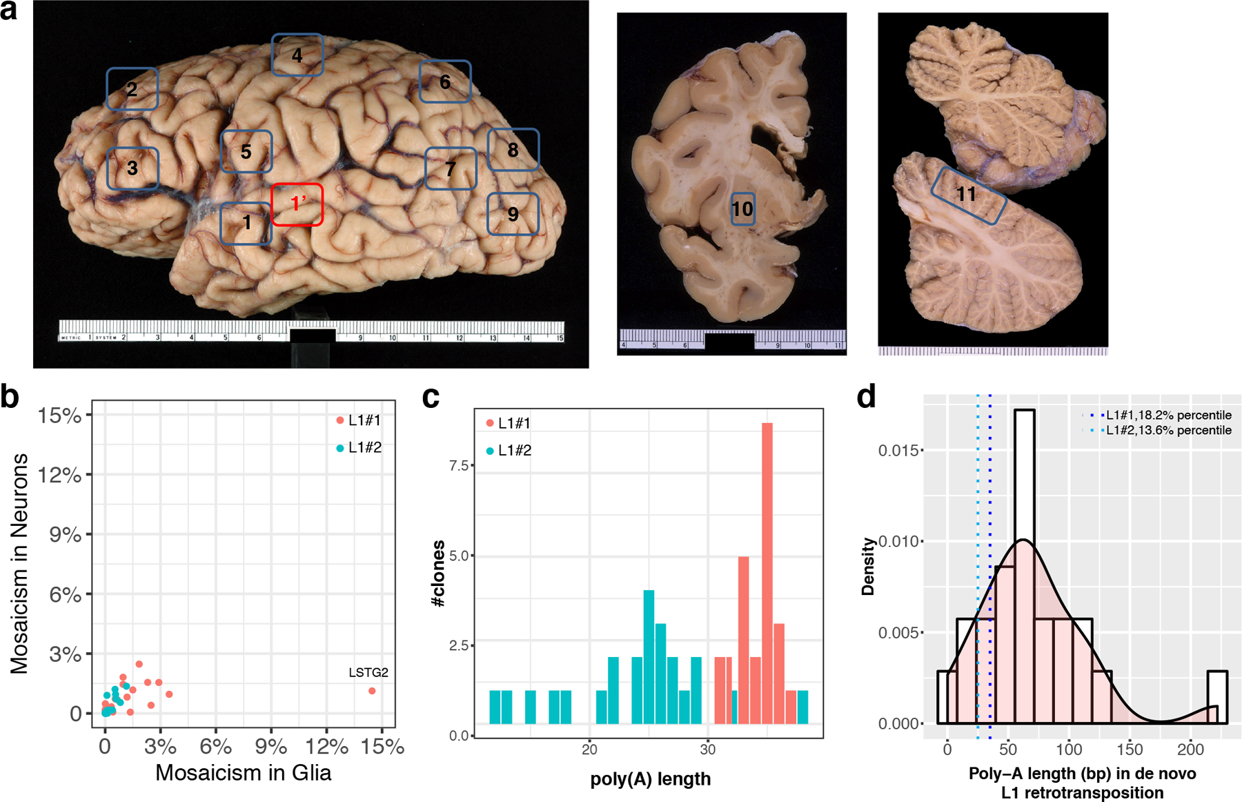
(a) Anatomical brain regions studied in donor 12004: 1 and 1’, superior temporal gyrus (BA22, both sides); 2, prefrontal cortex distal (BA9, both sides); 3, prefrontal cortex proximal (BA46, both sides); 4, motor cortex distal (BA4, both sides); 5, motor cortex proximal (BA6, both sides); 6, parietal cortex distal (BA7, both sides); 7, parietal cortex proximal (BA39, both sides); 8, occipital cortex distal (BA19, both sides); 9, occipital cortex proximal (BA19, both sides); 10, putamen (both sides); 11, cerebellum (both sides). The tissue for deep whole genome sequencing is from right superior temporal gyrus (1’). The tissues that were dissected from both hemispheres were bilaterally symmetrical. The metric unit on the ruler is the centimeter. (b) The levels of mosaicism in neurons are highly correlated with levels in glia. Red, L1#1; green, L1#2. (c) Poly(A) lengths of L1#1 and L1#2 were estimated as the lengths supported by the highest numbers of GL1#1 and GL1#2 clones (see Supplementary 8b). The variation among clones was likely the result of PCR stutter around low-complexity templates⁶⁸. (d) Poly-A length distribution in 22 previously reported de novo and disease-causing L1 retrotranspositions. The poly-A lengths of L1#1 and L1#2 are at 18.2% and 13.6% percentiles, respectively, of this distribution.

Extended Data Fig. 9. The genomic locus with L1#1 insertion.

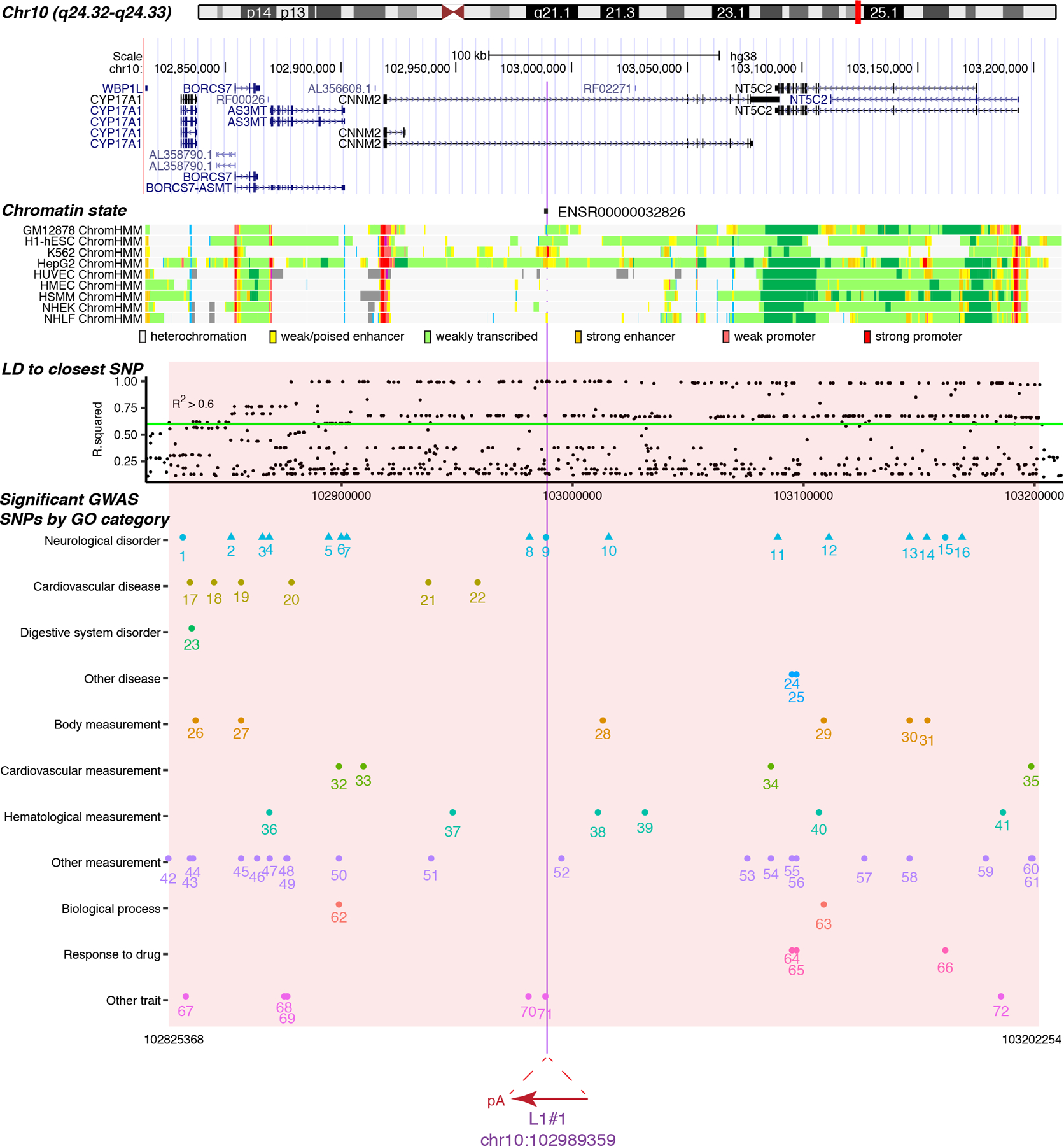
Supplementary Fig. 13. L1#1 is inserted in a 2.6kb promoter flanking region (ENSR00000032826) that is hypothesized to regulates the expression of nearby genes⁶⁹. The chromatin states are shown for a subset of human cell lines: light gray, heterochromatin; light green, weakly transcribed; yellow, weak/poised enhancer; orange, strong enhancer; light red, weak promoter; bright red, strong promoter. L1#1 is inserted in a linkage disequilibrium (LD) block, based on the common SNPs that are highly correlated (R2 > 0.6, green line) with the closest common SNP to L1#1, rs1890185. This LD block is highlighted in red, and contains 72 lead SNPs associated with 10 diseases or disorders and 28 measurements or other traits⁷⁰, including 13 risk SNPs from 11 schizophrenia studies (triangle). We categorized all traits under 11 terms based on the Experimental Factor Ontology⁷¹. The significantly associated SNPs, indexed from number 1 to 72, are documented in details in Supplementary Table 6.

Extended Data Fig. 10. Fluorescence quantification in the reporter assay.

(a-b) Original photos of the representative images in Fig. 6d and 6e. (c) Raw fluorescence intensities (green and red) used in the statistical analysis in Fig. 6f and Fig. 6g were in the range of 0–3035 for green fluorescence and 0–3613 for red, with no saturated pixels (>4000). Each cell is represented by the average pixel intensity (dot) and the maximum and minimum pixel intensities (bar). Red, Gcont#1; Cyan, GL1#1; Green, Gcont#2; Purple, GL1#2. (d) Measurement of the green fluorescence, red fluorescence and brightfield of three cells. C1, live cell; C2, dead cell, C3, dead cell. Each image is a representative of the green and red fluorescence images in well 1 to well 5 for any reporters (total=60). (e) Representative images from each the GFP fluorescence of the control and L1#1 reporters in the single transfection experiment (2 wells and 3 images per well, see Fig. 6c). The maximum signal intensities are adjusted from 4095 to 1000 in (d) and (e) to illustrate the cells with weak fluorescence.

Members of The Brain Somatic Mosaicism Network

Xiaowei Zhu¹, Bo Zhou¹, Alexander Urban¹, Christopher Walsh², Javier Ganz², Mollie Woodworth², Pengpeng Li², Rachel Rodin², Robert Hill², Sara Bizzotto², Zinan Zhou², Alice Lee³, Alissa D'Gama³, Alon Galor³, Craig Bohrson³, Daniel Kwon³, Doga Gulhan³, Elaine Lim³, Isidro Cortes³, Joe Luquette³, Maxwell Sherman³, Michael Coulter³, Michael Lodato³, Peter Park³, Rebeca Monroy³, Sonia Kim³, Yanmei Dou³, Andrew Chess⁴, Attila Jones⁴, Chaggai Rosenbluh⁴, Schahram Akbarian⁴, Ben Langmead⁵, Jeremy Thorpe⁵, Jonathan Pevsner⁵, Rob Scharpf⁵, Sean Cho⁵, Flora Vaccarino⁶, Liana Fasching⁶, Simone Tomasi⁶, Nenad Sestan⁶, Sirisha Pochareddy⁶, Andrew Jaffe⁷, Apua Paquola⁷, Daniel Weinberger⁷, Jennifer Erwin⁷, Jooheon Shin⁷, Richard Straub⁷, Rujuta Narurkar⁷, Anjene Addington⁸, David Panchision⁸, Doug Meinecke⁸, Geetha Senthil⁸, Lora Bingaman⁸, Tara Dutka⁸, Thomas Lehne⁸, Alexej Abyzov⁹, Taejeong Bae⁹, Laura Saucedo-Cuevas¹⁰, Tara Conniff¹⁰, Diane A. Flasch¹¹, Trenton J. Frisbie¹¹, Jeffrey M. Kidd¹¹, Mandy M. Lam¹¹, John B. Moldovan¹¹, John V. Moran¹¹, Kenneth Y. Kwan¹¹, Ryan E. Mills¹¹, Sarah Emery¹¹, Weichen Zhou¹¹, Yifan Wang¹¹, Kenneth Daily¹², Mette Peters¹², Fred Gage¹³, Meiyan Wang¹³, Patrick Reed¹³, Sara Linker¹³, Ani Sarkar¹³, Aitor Serres¹⁴, David Juan¹⁴, Inna Povolotskaya¹⁴, Irene Lobon¹⁴, Manuel Solis¹⁴, Raquel Garcia¹⁴, Tomas Marques-Bonet¹⁴, Gary Mathern¹⁵, Eric Courchesne¹⁶, Jing Gu¹⁶, Joseph Gleeson¹⁶, Laurel Ball¹⁶, Renee George¹⁶, Tiziano Pramparo¹⁶, Aakrosh Ratan¹⁷, Mike J. McConnell¹⁷

¹Stanford University, Palo Alto, CA. ²Boston Children's Hospital, Boston, MA. ³Harvard University, Boston, MA. ⁴Icahn School of Medicine at Mt. Sinai, New York, NY. ⁵Kennedy Krieger Institute, Baltimore, MD. ⁶Yale University, New Haven, CT. ⁷Lieber Institute for Brain Development, Baltimore, MD. ⁸National Institute of Mental Health, Bathesda, MD. ⁹Mayo Clinic, Rochester, MN. ¹⁰Rockefeller University, New York, NY. ¹¹University of Michigan, Ann Arbor, MI. ¹²Sage Bionetworks, Seattle, WA. ¹³Salk Institute for Biological Studies, La Jolla, CA. ¹⁴Universitat Pompeu Fabra, Barcelona, Spain. ¹⁵University of California, Los Angeles, Los Angeles, CA. ¹⁶University of California, San Diego, San Diego, CA. ¹⁷University of Virginia, Charlottesville, VA.

References

- 1.Luan DD, Korman MH, Jakubczak JL & Eickbush TH Reverse transcription of R2Bm RNA is primed by a nick at the chromosomal target site: A mechanism for non-LTR retrotransposition. Cell 72, 595–605 (1993). [DOI] [PubMed] [Google Scholar]
- 2.Symer DE et al. Human l1 retrotransposition is associated with genetic instability in vivo. Cell 110, 327–338 (2002). [DOI] [PubMed] [Google Scholar]
- 3.Hancks DC & Kazazian HH Roles for retrotransposon insertions in human disease. Mob. DNA 7, (2016). [DOI] [PMC free article] [PubMed] [Google Scholar]
- 4.Tubio JMC et al. Extensive transduction of nonrepetitive DNA mediated by L1 retrotransposition in cancer genomes. Science 345, (2014). [DOI] [PMC free article] [PubMed] [Google Scholar]
- 5.Evrony GD et al. Cell Lineage Analysis in Human Brain Using Endogenous Retroelements. Neuron 85, 49–60 (2015). [DOI] [PMC free article] [PubMed] [Google Scholar]
- 6.Erwin JA et al. L1-associated genomic regions are deleted in somatic cells of the healthy human brain. Nat. Neurosci 19, 1583–1591 (2016). [DOI] [PMC free article] [PubMed] [Google Scholar]
- 7.Reilly MT, Faulkner GJ, Dubnau J, Ponomarev I & Gage FH The Role of Transposable Elements in Health and Diseases of the Central Nervous System. J. Neurosci 33, 17577–17586 (2013). [DOI] [PMC free article] [PubMed] [Google Scholar]
- 8.Jacob-Hirsch J. et al. Whole-genome sequencing reveals principles of brain retrotransposition in neurodevelopmental disorders. Cell Res 28, 187–203 (2018). [DOI] [PMC free article] [PubMed] [Google Scholar]
- 9.Muotri AR et al. Somatic mosaicism in neuronal precursor cells mediated by L1 retrotransposition. Nature 435, 903–910 (2005). [DOI] [PubMed] [Google Scholar]
- 10.Richardson SR et al. Heritable L1 retrotransposition in the mouse primordial germline and early embryo. Genome Res 27, 1395–1405 (2017). [DOI] [PMC free article] [PubMed] [Google Scholar]
- 11.Sanchez-Luque FJ et al. LINE-1 Evasion of Epigenetic Repression in Humans. Mol. Cell 75, 590–604.e12 (2019). [DOI] [PubMed] [Google Scholar]
- 12.Baillie JK et al. Somatic retrotransposition alters the genetic landscape of the human brain. Nature 479, 534–537 (2011). [DOI] [PMC free article] [PubMed] [Google Scholar]
- 13.Upton KR et al. Ubiquitous L1 mosaicism in hippocampal neurons. Cell 161, 228–239 (2015). [DOI] [PMC free article] [PubMed] [Google Scholar]
- 14.Evrony GD et al. Single-neuron sequencing analysis of l1 retrotransposition and somatic mutation in the human brain. Cell 151, 483–496 (2012). [DOI] [PMC free article] [PubMed] [Google Scholar]
- 15.Evrony GD, Lee E, Park PJ & Walsh CA Resolving rates of mutation in the brain using single-neuron genomics. Elife 5, 1–32 (2016). [DOI] [PMC free article] [PubMed] [Google Scholar]
- 16.Zhou W et al. Identification and characterization of occult human-specific LINE-1 insertions using long-read sequencing technology. (2019). doi: 10.1093/nar/gkz1173 [DOI] [PMC free article] [PubMed]
- 17.Rishishwar L, Mariño-Ramírez L & Jordan IK Benchmarking computational tools for polymorphic transposable element detection. Brief. Bioinform 18, 908–918 (2017). [DOI] [PMC free article] [PubMed] [Google Scholar]
- 18.Keane TM, Wong K & Adams DJ RetroSeq: Transposable element discovery from next-generation sequencing data. Bioinformatics 29, 389–390 (2013). [DOI] [PMC free article] [PubMed] [Google Scholar]
- 19.Birur B, Kraguljac NV, Shelton RC & Lahti AC Brain structure, function, and neurochemistry in schizophrenia and bipolar disorder—a systematic review of the magnetic resonance neuroimaging literature. npj Schizophr 3, 15 (2017). [DOI] [PMC free article] [PubMed] [Google Scholar]
- 20.Eberle MA et al. A reference data set of 5.4 million phased human variants validated by genetic inheritance from sequencing a three-generation 17-member pedigree. Genome Res 27, 157–164 (2017). [DOI] [PMC free article] [PubMed] [Google Scholar]
- 21.Flasch DA et al. Genome-wide de novo L1 Retrotransposition Connects Endonuclease Activity with Replication. Cell 1–15 (2019). doi: 10.1016/j.cell.2019.02.050 [DOI] [PMC free article] [PubMed]
- 22.Breiman L. Random Forests. Mach. Learn 45, 5–32 (2001). [Google Scholar]
- 23.Skowronski J, Fanning TG & Singer MF Unit-length line-1 transcripts in human teratocarcinoma cells. Mol. Cell. Biol 8, 1385–97 (1988). [DOI] [PMC free article] [PubMed] [Google Scholar]
- 24.Moran JV et al. Exon Shuffling by L1 Retrotransposition. Science 283, 1530–1534 (1999). [DOI] [PubMed] [Google Scholar]
- 25.Bae T. et al. Different mutational rates and mechanisms in human cells at pregastrulation and neurogenesis. Science 359, 550–555 (2018). [DOI] [PMC free article] [PubMed] [Google Scholar]
- 26.Ovchinnikov I et al. Genomic Characterization of Recent Human LINE-1 Insertions: Evidence Supporting Random Insertion Genomic Characterization of Recent Human LINE-1 Insertions: Evidence Supporting Random Insertion 2050–2058 (2001). doi: 10.1101/gr.194701 [DOI] [PMC free article] [PubMed]
- 27.Morrish TA et al. DNA repair mediated by endonuclease-independent LINE-1 retrotransposition. Nat. Genet 31, 159–165 (2002). [DOI] [PubMed] [Google Scholar]
- 28.McConnell MJ et al. Intersection of diverse neuronal genomes and neuropsychiatric disease: The Brain Somatic Mosaicism Network. Science 356, (2017). [DOI] [PMC free article] [PubMed] [Google Scholar]
- 29.Feng Q, Moran JV, Kazazian HH & Boeke JD Human L1 retrotransposon encodes a conserved endonuclease required for retrotransposition. Cell 87, 905–916 (1996). [DOI] [PubMed] [Google Scholar]
- 30.Grimaldi G, Skowronski J & Singer MF Defining the beginning and end of KpnI family segments. EMBO J 3, 1753–1759 (1984). [DOI] [PMC free article] [PubMed] [Google Scholar]
- 31.Zingler N. et al. Analysis of 5’ junctions of human LINE-1 and Alu retrotransposons suggests an alternative model for 5’-end attachment requiring microhomology-mediated end-joining. Genome Res 15, 780–789 (2005). [DOI] [PMC free article] [PubMed] [Google Scholar]
- 32.Zerbino DR, Wilder SP, Johnson N, Juettemann T & Flicek PR The Ensembl Regulatory Build. Genome Biol 16, 1–8 (2015). [DOI] [PMC free article] [PubMed] [Google Scholar]
- 33.Ripke S. et al. Biological insights from 108 schizophrenia-associated genetic loci. Nature 511, 421–427 (2014). [DOI] [PMC free article] [PubMed] [Google Scholar]
- 34.Han JS, Szak ST & Boeke JD Transcriptional disruption by the L1 retrotransposon and implications for mammalian transcriptomes. Nature 429, 268–274 (2004). [DOI] [PubMed] [Google Scholar]
- 35.Dou Y. et al. Accurate detection of mosaic variants in sequencing data without matched controls. Nature Biotechnology (2020). doi: 10.1038/s41587-019-0368-8 [DOI] [PMC free article] [PubMed]
- 36.Scott EC & Devine SE The role of somatic L1 retrotransposition in human cancers. Viruses (2017). doi: 10.3390/v9060131 [DOI] [PMC free article] [PubMed]
- 37.Malatesta P, Hartfuss E & Götz M. Isolation of radial glial cells by fluorescent-activated cell sorting reveals a neuronal lineage. Development 127, 5253–5263 (2000). [DOI] [PubMed] [Google Scholar]
- 38.Coufal NG et al. L1 retrotransposition in human neural progenitor cells. Nature 460, 1127–1131 (2009). [DOI] [PMC free article] [PubMed] [Google Scholar]
- 39.Rehen SK et al. Chromosomal variation in neurons of the developing and adult mammalian nervous system. Proc. Natl. Acad. Sci. U. S. A 98, 13361–13366 (2001). [DOI] [PMC free article] [PubMed] [Google Scholar]
- 40.De Cecco M. et al. L1 drives IFN in senescent cells and promotes age-associated inflammation. Nature 566, 73–78 (2019). [DOI] [PMC free article] [PubMed] [Google Scholar]
- 41.Jacob-Hirsch J. et al. Whole-genome sequencing reveals principles of brain retrotransposition in neurodevelopmental disorders. Cell Res 28, 187–203 (2018). [DOI] [PMC free article] [PubMed] [Google Scholar]
- 42.Yamaguchi Y & Miura M. Programmed cell death in neurodevelopment. Dev. Cell 32, 478–490 (2015). [DOI] [PubMed] [Google Scholar]
- 43.Shirley MD et al. Sturge–Weber Syndrome and Port-Wine Stains Caused by Somatic Mutation in. N. Engl. J. Med 368, 1971–1979 (2013). [DOI] [PMC free article] [PubMed] [Google Scholar]
- 44.Lim JS et al. Brain somatic mutations in MTOR cause focal cortical dysplasia type II leading to intractable epilepsy. Nat. Med 21, 395 (2015). [DOI] [PubMed] [Google Scholar]
- 45.Poduri A. et al. Somatic Activation of AKT3 Causes Hemispheric Developmental Brain Malformations. Neuron 74, 41–48 (2012). [DOI] [PMC free article] [PubMed] [Google Scholar]
- 46.Thyme SB et al. Phenotypic Landscape of Schizophrenia-Associated Genes Defines Candidates and Their Shared Functions. Cell (2019). [DOI] [PMC free article] [PubMed]
- 47.Fine D. et al. A syndrome of congenital microcephaly, intellectual disability and dysmorphism with a homozygous mutation in FRMD4A. Eur. J. Hum. Genet 23, 1729–1734 (2015). [DOI] [PMC free article] [PubMed] [Google Scholar]
- 48.Rees E. et al. Analysis of copy number variations at 15 schizophrenia-associated loci. Br. J. Psychiatry 204, 108–114 (2014). [DOI] [PMC free article] [PubMed] [Google Scholar]
- 49.Lek M. et al. Analysis of protein-coding genetic variation in 60,706 humans. Nature 536, 285–291 (2016). [DOI] [PMC free article] [PubMed] [Google Scholar]
- 50.Ikenouchi J & Umeda M. FRMD4A regulates epithelial polarity by connecting Arf6 activation with the PAR complex. Proc. Natl. Acad. Sci 107, 748–753 (2010). [DOI] [PMC free article] [PubMed] [Google Scholar]
Methods-only References
- 51.Stan AD et al. Magnetic resonance spectroscopy and tissue protein concentrations together suggest lower glutamate signaling in dentate gyrus in schizophrenia. Mol. Psychiatry 20, 433–439 (2015). [DOI] [PubMed] [Google Scholar]
- 52.Matevossian A & Akbarian S. Neuronal Nuclei Isolation from Human Postmortem Brain Tissue. J. Vis. Exp 4–5 (2008). doi: 10.3791/914 [DOI] [PMC free article] [PubMed]
- 53.Kozlenkov A. et al. A unique role for DNA (hydroxy)methylation in epigenetic regulation of human inhibitory neurons. Sci. Adv (2018). doi: 10.1126/sciadv.aau6190 [DOI] [PMC free article] [PubMed]
- 54.Julius MH, Masuda T & Herzenberg LA Demonstration That Antigen-Binding Cells Are Precursors of Antibody-Producing Cells After Purification with a Fluorescence-Activated Cell Sorter. Proc. Natl. Acad. Sci. U. S. A 69, 1934–1938 (1972). [DOI] [PMC free article] [PubMed] [Google Scholar]
- 55.Zhang Y. et al. Purification and Characterization of Progenitor and Mature Human Astrocytes Reveals Transcriptional and Functional Differences with Mouse. Neuron 89, 37–53 (2016). [DOI] [PMC free article] [PubMed] [Google Scholar]
- 56.Sudmant PH et al. An integrated map of structural variation in 2,504 human genomes. Nature 526, 75–81 (2015). [DOI] [PMC free article] [PubMed] [Google Scholar]
- 57.Li H & Durbin R. Fast and accurate short read alignment with Burrows-Wheeler transform. Bioinformatics 25, 1754–1760 (2009). [DOI] [PMC free article] [PubMed] [Google Scholar]
- 58.Jurka J. Repbase Update: a database and an electronic journal of repetitive elements. Trends Genet 16, 418–420 (2000). [DOI] [PubMed] [Google Scholar]
- 59.Wootton JC Non-globular domains in protein sequences: Automated segmentation using complexity measures. Comput. Chem 18, 269–285 (1994). [DOI] [PubMed] [Google Scholar]
- 60.Friedman JH, Hastie T & Tibshirani R. Regularization Paths for Generalized Linear Models via Coordinate Descent. J. Stat. Softw 33, 1–22 (2010). [PMC free article] [PubMed] [Google Scholar]
- 61.Liaw A & Wiener M. Classification and Regression by randomForest. R news 2, 18–22 (2002). [Google Scholar]
- 62.Robin X. et al. pROC: An open-source package for R and S+ to analyze and compare ROC curves. BMC Bioinformatics 12, (2011). [DOI] [PMC free article] [PubMed] [Google Scholar]
- 63.Robinson JT et al. Integrative genomics viewer. Nat. Biotechnol 29, 24–26 (2011). [DOI] [PMC free article] [PubMed] [Google Scholar]
- 64.Zhou B et al. Detection and quantification of mosaic genomic dna variation in primary somatic tissues using ddPCR: analysis of mosaic transposable-element insertions, copy-number variants, and single-nucleotide variants. in Digital PCR: Methods and Protocols (eds. Karlin-neumann G & Francisco B) 1768, 173–190 (SPringer Science+Business Media, New York, 2018). [DOI] [PubMed] [Google Scholar]
- 65.Szak ST et al. Molecular archeology of L1 insertions in the human genome. Genome Biol 3, research00521–18 (2002). [DOI] [PMC free article] [PubMed] [Google Scholar]
- 66.Heckman KL & Pease LR Gene splicing and mutagenesis by PCR-driven overlap extension. Nat. Protoc 2, 924–932 (2007). [DOI] [PubMed] [Google Scholar]
- 67.Bonano VI, Oltean S & Garcia-blanco MA A protocol for imaging alternative splicing regulation in vivo using fluorescence reporters in transgenic mice. Nat. Protoc 2, 2166–2181 (2007). [DOI] [PubMed] [Google Scholar]
- 68.Shinde D, Lai Y, Sun F & Arnheim N. Taq DNA polymerase slippage mutation rates measured by PCR and quasi-likelihood analysis: (CA/GT)nand (A/T)nmicrosatellites. Nucleic Acids Res 31, 974–980 (2003). [DOI] [PMC free article] [PubMed] [Google Scholar]
- 69.Zerbino DR et al. Ensembl regulation resources. Database 2016, 1–13 (2016). [DOI] [PMC free article] [PubMed] [Google Scholar]
- 70.McMahon A. et al. The NHGRI-EBI GWAS Catalog of published genome-wide association studies, targeted arrays and summary statistics 2019. Nucleic Acids Res 47, D1005–D1012 (2018). [DOI] [PMC free article] [PubMed] [Google Scholar]
- 71.Malone J. et al. Modeling sample variables with an Experimental Factor Ontology. Bioinformatics 26, 1112–1118 (2010). [DOI] [PMC free article] [PubMed] [Google Scholar]
Associated Data
This section collects any data citations, data availability statements, or supplementary materials included in this article.
Supplementary Materials
Data Availability Statement