Mass spectrometry and proteome analysis to identify SARS-CoV-2 protein from COVID-19 patient swab samples

Summary

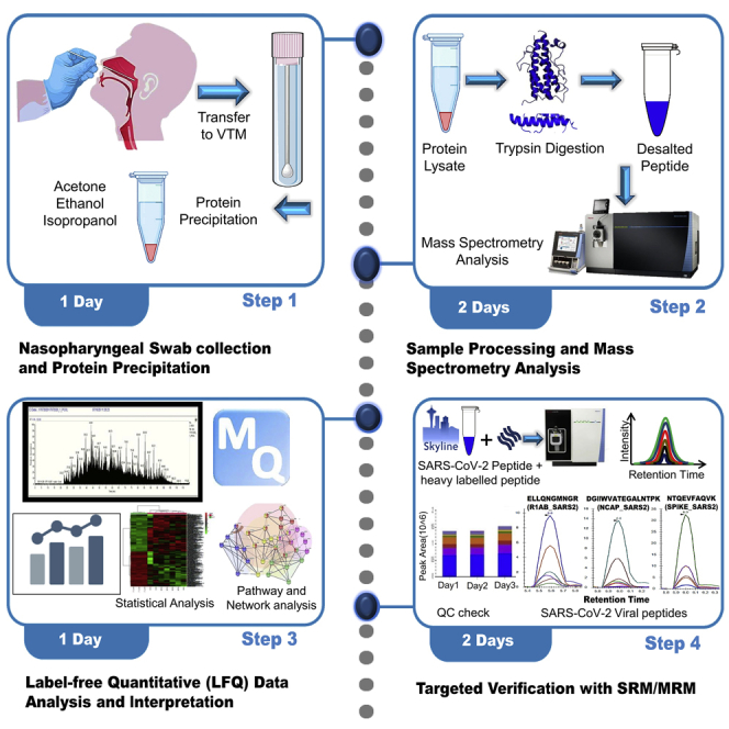
With new emerging SARS-CoV-2 strains and their increased pathogenicity, diagnosis has become more challenging. Molecular diagnosis often involves the use of nasopharyngeal swabs and subsequent real-time PCR-based tests. Although this test is the gold standard, it has several limitations; therefore, more complementary assays are required. This protocol describes how to identify SARS-CoV-2 protein from patients' nasopharyngeal swab samples. We first introduce the approach of label-free quantitative proteomics. We then detail target verification by triple quadrupole mass spectrometry (MS)-based targeted proteomics.

For complete details on the use and execution of this profile, please refer to Bankar et al. (2021).

Graphical abstract

Highlights

• •A protocol for identification of SARS-CoV-2 protein from patients' swab samples
• •Sequential steps involved in proteomic sample preparation are elaborated
• •Detailed procedure for MS-based targeted proteomic verification is presented
• •A detailed presentation of workflow for label-free and targeted data analyses

With new emerging SARS-CoV-2 strains and their increased pathogenicity, diagnosis has become more challenging. Molecular diagnosis often involves the use of nasopharyngeal swabs and subsequent real-time PCR-based tests. Although this test is the gold standard, it has several limitations; therefore, more complementary assays are required. This protocol describes how to identify SARS-CoV-2 protein from patients' nasopharyngeal swab samples. We first introduce the approach of label-free quantitative proteomics. We then detail target verification by triple quadrupole mass spectrometry (MS)-based targeted proteomics.

Before you begin

The study was approved by the Indian Institute of Technology (IIT), Bombay ethical committee, and Kasturba hospital for infectious diseases, Institutional Review Board.

Sample collection for deep proteome profiling

Timing: 1 day—Day 1

Timing: 4 h for step 1

• 1.
  Day 1: Procurement of Nasopharyngeal swab and viral inactivation

  • a.
    Swab Sample Collection for SARS-CoV-2

    • i.
      Collect nasopharyngeal Swab from COVID-19 suspected patients following complete biosafety protocol as per World Health Organization (WHO) and Indian Council of Medical Research (ICMR) guidelines.

      Note: This step to be performed by trained medical practitioners.

    • ii.
      For this, insert a sterile cotton swab into nostrils parallel to the palate, allowing it to absorb secretions and remove while slowly rotating.

      Note: Virus settled at the mucosal lining of the nasopharynx is thus picked-up on the swab while removing.

    • iii.
      Immediately immerse into sterile VTM (Viral Transport Media) (CDC, 2020).
    • iv.
      Keep 3 mL of total VTM in each tube and store at 4°C until a quantitative PCR test is performed (RT-PCR is currently considered the gold standard for SARS-CoV-2 detection).
    • v.
      Classify the swab samples into three categories based on RT-PCR screening: the positive samples, true negative samples and negative but recovered samples.

      Note: all the sample processing should be performed under the aseptic conditions of a BSL-2 facility as per WHO (World Health Organization) and ICMR (Indian Council of Medical Research) guidelines.

    • vi.
      Collect around 800 μL of the Swab+VTM mix in a sterile tube and incubate at 65°C for 45 min for heat inactivation of the virus.
    • vii.
      Aliquot 200 μL of heat-inactivated Swab+VTM mix in three sterile tubes and add 600 μL of acetone, ethanol, and isopropanol independently (one solvent per tube) and incubate at −20°C for 4 h.
    • viii.
      After incubation with the organic solvent, centrifuge the tubes at 15,000×g for 20 min at 4°C. Remove the supernatant using a micropipette without disturbing the protein precipitate.
    • ix.
      Further dry these precipitated protein pellets in the Laminar hood of BSL-2 and store at −80°C till further processing (the samples should be processed within a week).

      CRITICAL: If the samples are shipped from the hospital to the research center, they should be shifted in an aseptic container, thus minimizing the risk of contamination. All the activities such as aliquoting and processing should be done following biosafety guidelines in a BSL-2 laboratory.

Key resources table

REAGENT or RESOURCE	SOURCE	IDENTIFIER
Chemicals, peptides, and recombinant proteins
Acetone (HPLC grade)	Merck	SF2SF62425
Ethanol absolute	Merck	K51871183 942
Quick Start Bradford 1× Dye Reagent	Bio-Rad	5000205
Acetonitrile (ACN; MS grade)	Fisher Scientific	A/0620/21
Bovine Serum Albumin	HiMedia	TC194-25G
Calcium chloride	Fisher Scientific	BP510-500
Formic acid (FA; MS grade)	Fisher Scientific	147930250
Iodoacetamide	Sigma-Aldrich	1149-25G
Isopropanol (MS grade)	Fisher Scientific	Q13827
Magnesium Chloride	Fischer Scientific	BP214-500
Methanol (MS grade)	Fisher Scientific	A456-4
M.S. grade water	Pierce	51140
Phosphate Buffer Saline	HiMedia	TL1006-500ML
Sodium Chloride	Merck	DF6D661300
TCEP	Sigma-Aldrich	646547
Tris Base	Merck	648310
Trypsin (MS grade)	Pierce	90058
Urea	Merck	MB1D691237
Biological samples
Clinical samples from COVID-19 patients	Bankar et al. (2021)	For the characteristics see Table S1 from Bankar et al. (2021); Mendeley Data: https://doi.org/10.17632/rnfn3vhg63.1
Software and algorithms
MaxQuant	Tyanova et al. (2016)	MaxQuant v1.6.6.0
Metaboanalyst	Xia et al. (2015)	Metaboanalyst software V4
Reactome	Fabregat et al. (2018)	Reactome Version 73
Metascape	Zhou et al. (2019)	Metascape Version 3.5
STRING	Szklarczyk et al. (2019)	STRING Version 11
Skyline	MacLean et al. (2018)	Skyline Version 20.2.1.286
Deposited data
LFQ raw files and search output files for proteomics data sets	Bankar et al. (2021)	ProteomeXchange Consortium via the PRIDE partner repository: "PRIDE: PXD020580" and "PRIDE: PXD023016" https://www.ebi.ac.uk/pride/archive/projects/PXD023016 https://www.ebi.ac.uk/pride/archive/projects/PXD020580
Targeted proteomics data	Bankar et al. (2021)	Panorama Public: “https://panoramaweb.org/COVID_Swab_MRM.url”.
Additional supplemental items	Bankar et al. (2021)	Tables S1, S8 and S10 from Bankar et al. (2021); Mendeley Data: https://doi.org/10.17632/rnfn3vhg63.1.
Additional supplemental items	This paper	Table S4; Mendeley Data: DOI: https://doi.org/10.17632/ykx6jrpsm3.1 (https://data.mendeley.com/datasets/ykx6jrpsm3/1)
Other
Microtubes 1.5 mL	Axygen, A corning brand	MCT-150-C
BD™ Universal Viral Transport	Becton, Dickinson and Company	220239
PK20 EMPORE OCTADECYL C18 47MM	Merck	66883-U
Acclaim™ PepMap™ 100 C18 HPLC Columns	Thermo Scientific™	(P/N 164564)
PepMap TM RSLC C18 2 μm,100 Å, 75 μm∗50 cm	Thermo Scientific™	(P/N ES803A)
Hypersil Gold C18 column	Thermo Fisher Scientific	25002-102130
Micropipettes	Gilson	F167380
C18 material for in-house C18 tips	Merck Millipore	ZTC18M008
Zirconia/Silica beads	BioSpec products	11079110z
Pierce™ LTQ Velos ESI Positive Ion Calibration Solution	Thermo Scientific™	88323
Microplate reader (spectrophotometer)	Thermo Fisher Scientific	MultiSkan Go
pH meter	Eutech	CyberScan pH 510
Digital Shaking Drybath	Thermo Fisher Scientific	88880028
Orbitrap Fusion mass spectrometer	Thermo Fisher Scientific	FSN 10452
Nano LC	Thermo Fisher Scientific	EASY-nLC1200
TSQ Altis mass spectrometer	Thermo Fisher Scientific	TSQ02-10002
uHPLC - Vanquish	Thermo Fisher Scientific	VQF01-20001
Vacuum concentrator	Thermo Fisher Scientific	Savant ISS 110

Materials and equipment

Urea Lysis Buffer 8 M urea, 50 mM Tris, pH 8.0, 75 mM NaCl, 1 mM MgCl₂ for 50 mL (freshly prepared)

Reagent	Final concentration	Amount
Urea	8 M	30 mg
Tris	50 mM	3 mg
NaCl	75 mM	0.21 gms
MgCl2	1 mM	0.01 gms

Note: Initially, add all the regents to 30 mL of MilliQ water, maintain the pH 8, and make the volume 50 mL.

Note: Store at room temperature (R.T.°C) for 3 days. (Prepare fresh before beginning the experiment)

Dilution buffer (25 mM Tris pH 8.0, 1 mM CaCl₂)

Reagent	Final concentration	Amount
Tris	25 mM	151.2 gms
CaCl2	1 mM	7.2 gms

Note: Initially, add all the regents to 30 mL of MilliQ water, maintain the pH 8, and make the volume 50 mL.

Note: Store at R.T.°C for 3 days. (Prepare fresh before beginning the experiment)

Reagents for Mass Spectrometry (Discovery Study)

Solvents/buffer	Composition	Volume
Solvent A	0.1% Formic Acid	25 mL
Solvent B	80% ACN in 0.1% formic acid	25 mL
Wash Buffer	0.1% Formic Acid	50 mL
MilliQ Water	NA

Note: Store at R.T.°C, depending on experimental runs buffer are changed every 7 days.

Reagents for mass spectrometry (targeted study)

• •MRM sample Buffer

Reagent	Final concentration	Volume
Milli Q water	NA	1 mL
Formic Acid	0.1 %	1 µL

• •HPLC Buffer A

Reagent	Final concentration	Volume
Milli Q water	NA	1 Liter
Formic Acid	0.1 %	1 mL

• •HPLC Buffer B

Reagent	Final concentration	Volume
Acetonitrile	80 %	800 mL
Formic Acid	0.1 %	1 mL
Milli Q water	N/A	200 mL

• •HPLC Seal wash buffer

Reagent	Final concentration
Methanol	10 % (Milli Q water)

• •HPLC Needle Wash buffer

Reagent	Final concentration
Acetonitrile	50 % (Milli Q water)

Note: Store at R.T.°C. Generally the Buffer A and Buffer B used in uHPLC gets exhausted in 3–4 days and can be stored at R.T. Thus depending on experimental runs buffer are changed every 3–4 days. Whereas MRM sample buffer should be prepared fresh. HPLC seal and needle wash buffer can be replaced with fresh buffer in every 7 days.

Step-by-step method details

Discovery proteomics study for swab samples

Timing: 2 days—Day 2 and Day 3

Timing: 21 h for step 1

Timing: 4–6 h for step 2

Timing: 3–4 h, per sample, for step 3

Timing: 4–6 h for step 4

Timing: 2–4 h for step 5

Timing: 2 h for step 6

In the discovery proteomics study, label-free quantification (LFQ) is performed for the swab samples with an aim to identify the total number of proteins present in the swab samples. In LFQ experimental design, the proteins are trypsinized to generate peptides. These peptides are then analyzed using LC-MS/MS to generate raw data consisting of peptide sequences. These peptide sequences are then mapped to FASTA with suitable search engines such as Maxquant or Proteome Discoverer to identify the proteins. Further statistical and pathway analysis helped us to understand the significant and differential proteins expressed in each disease type contributing to their respective pathway and biology.

• 1.
  Day 2: Sample preparation for Label-Free-Quantification (LFQ) based mass spectrometry analysis

  • a.
    Dissolving the protein pellets in a suitable buffer

    • i.
      Add 75 μL of freshly prepared lysis buffer (8 M urea, 50 mM Tris, pH 8.0, 75 mM NaCl, 1 mM MgCl₂) to the protein pellet obtained from each solvent (acetone, ethanol and isopropanol).
    • ii.
      Dissolve the protein pellets in freshly prepared lysis buffer by vortexing.
    • iii.
      Pool the proteins extracted from solvents (i.e., Ethanol, Acetone and Isopropanol). Further, it can be stored at −80°C or processed immediately by in-solution digestion.

      Note: Urea buffer with Tris is used for lysis as Urea is a denaturant that helps to open the three-dimensional structure of proteins, which helps in digestion. This lysis buffer should be freshly prepared each time you begin your experiment. The pool of protein from Ethanol, Acetone and Isopropanol solvent extraction was made because the combination of these three yielded more SARS-CoV-2 unique peptides after in-solution digestion followed by mass spectrometry analysis (Table S1 and Figure S1).

  • b.
    Reduction and alkylation

    • i.
      Quantify the swab lysate mix by Bradford assay using Bovine Serum Albumin (BSA) protein to plot the standard curve (B. P. A. I. M. BIORAD, no date; Blagoev and Mann, 2006). The swab sample used in the study can have a concentration of ∼12μg/μL (total amount of protein ranges from 10–15 mg).
    • ii.
      Run the samples in 12% SDS-PAGE (P. G. E. BIORAD, no date; SDS-PAGE Gel, 2015) to check for the protein profile. One should obtain a clear protein profile in the gel before proceeding with in-solution digestion and mass spectrometry analysis (Figure S2).

      Note: SDS PAGE is run only for Quality Control purpose. The gel profile indicates whether the sample is good enough to take for digestion followed by Mass Spectrometric analysis, otherwise it will be detrimental for both columns and instrument.

      Optional: Samples should be loaded in duplicate. Use 10–15 μg of protein for Q.C. check.

    • iii.
      Place 30 μg of swab lysate in a fresh 1.5 mL Axygen tube for enzymatic digestion (make the final volume to 20 μL).
    • iv.
      Add 0.8 μL of 0.5 M TCEP (tris(2-carboxyethyl) phosphine solution, pH 7.0 for every 20 μL of swab lysate, to make final concentration of 20 mM.
    • v.
      Incubate swab lysate with TCEP at 37°C for 60 min for reduction of proteins.

      Note: i. Use Axygen 1.5 mL tubes (MCT-150-C), ii. Preferably use 1–10 μL high precision pipettes, iii. keep on non-shaking incubator at 37°C for 1 h.

    • vi.
      Add 1.6 μL of 0.5 M Iodoacetamide (IAA) solution for every 20 μL of swab lysate to make a final concentration of 40 mM and incubate at 37°C for 15 min in the dark.
  • c.
    In-solution digestion for generation of peptide

    • i.
      Dilute the alkylated sample by adding 4–5 volumes (60–80 μL) of dilution buffer (25 mM Tris pH 8.0, 1 mM CaCl₂) so that the final concentration of Urea is less than 1 M. This is required for optimal activity of trypsin.

      CRITICAL: Adjust pH of the solution to 8.0 with Sodium Hydroxide solution or HCl as per the supplier details. Check the pH using pH paper strip; use a drop of the sample on the paper and check the color as per the indicator.

    • ii.
      Digest the proteins by adding Pierce™ Trypsin Protease, MS Grade in 1:30 ratio (enzyme: protein) for 16 h at 37°C (Thermo Fisher, Digital Shaking Drybath - 500 rpm).

      Note: Preferably use 1–10 μL high precision pipettes for adding trypsin. Vortex briefly and give a short spin. Tap gently to remove air bubbles, if any.

• 2.Day 3: Quenching, peptide desalting, and peptide quantification

• a.
  Quenching of trypsinization reaction

  • i.
    Stop trypsin activity reaction by completely drying the samples in a Savant Speed Vac. Concentrator (ISS 110) set at medium heat (∼ 43°C).
• b.
  Preparation of in-house C18 desalting tips

  • i.
    Take a 20–200 μL (Tarson) tip and cut it below the mark.
  • ii.
    To prepare desalting tips, use the backside of a 10 μL tip to measure the amount of material (PK20 Empore Octadecyl C18 47 mm) required. DO NOT use material lower than this as it may not be sufficient to sit inside the tip well, resulting in loose packing and leakage.
  • iii.
    Pack the tip with the material properly by making the surface even from all sides. If this is not done, the material might not get activated evenly.
  • iv.
    Insert this tip into a 1.5 mL Eppendorf tube.

    Note: For further details of this protocol, one can refer these (Kumar et al., 2020; Ghantasala et al., 2021; Verma et al., 2021) and Figure S3.

    CRITICAL: Please DO NOT use sharp objects like a needle to make the C18 desalting tips. Insert the material heads-up into the tip. Peptide binding capacity of these in-house C18 tip depends upon the amount of C18 material used, the average loading volume can be 20–30 μL (∼30 μg), recovery volume is around 15–20 μL (∼15 μg) of peptide.

    Alternatives: Commercially available Millipore® Ziptips C18, pack of 96, Pierce™ C18 Tips, 10 μL bed can be used as an alternative to these tips

• c.
  In-house C18 tips desalting protocol: Activation

  • i.
    Pass 40 μL of 50% acetonitrile (ACN) with 0.1% formic acid (F.A.) three times from the in-house C18 tip (tip containing C18 material which is freshly prepared for peptide desalting from step (2.b). Centrifuge at 1500×g for 1 min (i.e., 40 μL, 1 min, 1500×g) to pass the solution through the tips.
  • ii.
    Pass 99.9% ACN in 0.1% FA; 40 μL, 1 min, 1500×g. Repeat this step 3 times.

    Note: Pass 99.9% ACN in 0.1% F.A.; 40 μL, 3 times simultaneously for activating the C18 material present in the in-house C18 tip and the eluent is discarded each time.

• d.
  In-house C18 tips desalting protocol: Equilibration

  • i.
    Pass 0.1% F.A. in Milli-Q water; 40 μL, 1 min, 1500×g. Repeat this step 3 times.
  • ii.
    Discard the remaining solvent with a syringe and insert the tip into a 1.5 mL sample tube.

    Note: As the peptide sample is reconstituted in the 0.1% F.A. in Milli-Q, C18 material in the in-house C18 tip is washed with 0.1% F.A. in Milli-Q water to equilibrate the in-house C18 tip with the sample buffer.

• e.
  In-house C18 tips desalting protocol: Sample passing

  • i.
    Reconstitute the peptide sample in an appropriate volume (preferably 40 μL) of Milli Q water with 0.1% F.A. and add to the activated tip, which is passed through the tip by centrifugation for 1 min at 1000×g. The eluted peptide solution is again passed through the same in-house C18 tip (by centrifugation) at least 6 times (Figure S3).

    Note: Here, the eluted peptide was reapplied and repeatedly passed through C18 material of the in-house C18 tip to maximize the binding of peptides with the C18 material

• f.
  In-house C18 tips desalting protocol: Sample cleaning

  • i.
    Pass Milli Q water with 0.1% F.A.; 40 μL, 1 min, 1500×g. Repeat this step 3 times.
  • ii.
    Discard the remaining solvent with a syringe and insert the tip into a fresh 1.5 mL tube.

    Note: Here, 0.1% F.A. was passed with the C18 material of the in-house C18 tip to remove and wash the unwanted salts present in the peptide solution.

• g.
  In-house C18 tips desalting protocol: Sample elution

  • i.
    Pass 50% ACN in 0.1% FA; 60 μL, 1 min, 1000×g. Repeat this step 3 times. Fresh ACN aliquot is used each time and the elute was collectively pooled.
  • ii.
    Pass 70% ACN in 0.1% F.A.; 60 μL, 3 min, 4000×g and pool the eluent with the eluent obtained from step (2. g.i).
  • iii.
    After pooled eluent is obtained from passing 50% ACN and 70% ACN elution, dry the eluent with Savant speed-vac (ISS 110) at low-temperature mode.

    Note: Once you have passed the peptide solution 6 times and washed the in-house C18 tip with 0.1% F.A. to remove the debris, pass 50% and 70% ACN in 0.1% F.A., sequentially to elute the peptides binding to the C18 material of the in-house C18 tip (Figure S3).(Kumar et al., 2020; Ghantasala et al., 2021; Verma et al., 2021).

• h.
  Quantification of peptides

  • i.
    Reconstitute cleaned peptides in 15 μL of 0.1 % (v/v) formic acid (FA) in MQ water. Take the absorbance at 205 and 280 nm (e.g., using MultiSkan GO, Thermo Fisher Scientific).
  • ii.
    Estimate the peptide concentration using the Scopes method (Scopes, 1974; Anthis and Clore, 2013).
  • iii.
    Take 1 μg of peptide forward for the mass spectrometry analysis.

    Note: Final peptide concentration is made to 0.25 μg/μL and 4 μL of peptide solution is injected into the nLC

• 3.
  Day 3: Sample analysis with Mass Spectrometry (Discovery Proteomics Study)

  • a.
    Instrumental Quality Assessment and Quality check

    • i.
      Use a high resolution mass spectrometer to perform the deep proteomic analysis of thus prepared peptide samples.

      Note: We have used Orbitrap Fusion™ coupled to EASY-nLC™ 1200 System for the discovery proteomic analysis of COVID-19 swab samples.

    • ii.
      Calibrate the instrument, as per requirement.

      Note: Both MS and MS/MS calibration should be carried out at the regular intervals (monthly and at the beginning of a new batch of an experiment). For Orbitrap Fusion calibration was done with Pierce™ LTQ Velos ESI Positive Ion Calibration Solution - which includes caffeine (2 μg/mL), MRFA (1 μg/mL), Ultramark 1621 (0.001%) and n-butylamine (0.0005%) in an aqueous solution of acetonitrile (50%), methanol (25%) and acetic acid (1%) - as per manufacturer's instructions (Catalog, 2015).

  • b.
    Nanospray columns

    Note: The column outline from the L.C. is connected to the precolumn/trap column using Viper union, the trap column is connected to the Analytical column using Mixing / Venting Tee (Fisher Scientific Inc, 2013). The analytical column is then placed near to sweep cone and Ion transfer capillary with the EASY-Spray NG source (Figure S4).

    • i.
      For the above mentioned setup, use precolumn Acclaim PepMap TM 100, 100 μm∗2 cm, nanoviper C18, 5 μm,100 Å.

      Note: Precolumn is mainly involved in conditioning the mobile phase before it reaches to the analytical column of nanoLC.

    • ii.
      For the Analytical column, use PepMap TM RSLC C18 2 μm,100 Å, 75 μm∗50 cm.

      Note: Analytical column is generally involved in qualitative analysis and results in fractionation of peptide samples according to their hydrophobicity.

  • c.
    Liquid Chromatography System used for Discovery Proteomics Study

    • i.
      Thermo EASY-nLC™ 1200 System has been used for the discovery phase proteomics, operated at a flow rate of 300 nL/min.
    • ii.
      Solvent A is composed of 0.1% F.A. in M.S. grade water, and solvent B comprises 80% ACN with 0.1% F.A. in M.S. grade water.
    • iii.
      Use an L.C. gradient of 120 min to separate peptides on the nLC column.
    • iv.
      Solvent B increased from 5 to 30% from the 5^th min to the 80^th min of the run, followed by an increase to 60% and then to 90% till 115^th min. Solvent B is maintained at 90% for the last 5 min (Table 1; Figure 1).
  • d.
    M.S. parameters and data acquisition

    • i.
      Keep the peptide samples obtained from the in-solution digestion of the swab protein pool (i.e., Ethanol, Acetone, and Isopropanol) in the nano-LC autosampler maintained at 8°C and analyze the sample by using LC-MS setup as per parameters mentioned in Table S2.
    • ii.
      Inject one μg (0.25 μg/μL) of the peptide for the 120 min analysis on is subjected Orbitrap Fusion™ in ddMS² OT HCD mode (Table S2) for spectral acquisition (Figure 2).

      Note: Technical replicates for Mass spectrometry runs of individual samples were not performed. However, the individual samples in each cohort were considered as biological replicates. Samples were randomly run for discovery analysis and for targeted verification study. Blanks were run after each sample to ensure that there was no carryover from one sample to another.

• 4.Day 3: MaxQuant analysis of swab samples
  Save the mass spectrometric raw files (.raw) generated after mass spectrometry in a folder named DD-MM-YY format for the protein identification by MaxQuant coupled with the Andromeda search engine.

  • a.
    MaxQuant analysis

    • i.
      Analyze the raw datasets by using MaxQuant (v1.6.6.0) (Tyanova et al., 2016) with the Human SwissProt and severe acute respiratory syndrome coronavirus 2 (SARS-CoV-2) SwissProt database and perform the downstream analysis as described in the quantification and statistical analysis section. Readers are also encouraged to follow the latest software guidelines from MaxQuant (https://maxquant.org/) (Tyanova et al., 2015).

      Note: Reader can go through the given link for detailed workflow for MaxQuant analysis (http://coxdocs.org/doku.php?id=maxquant:manual:beginner) and for training purposes, user can visit YouTube Videos available from MaxQuant (https://maxquant.org/summer_school/).

      CRITICAL: For this study, we used the Human and SARS-CoV-2 SwissProt database, which contains more than 20,300 and 13 proteins, respectively (Bankar et al., 2021). Users can parallelly use other search engines like MASCOT, Sequest HT, MS Amanda (Dorfer et al., 2014) integrated into Proteome Discoverer (Orsburn, 2021), Sequest, Mascot and Comet integrated into Trans-Proteomic Pipeline (TPP) (Deutsch et al., 2015) etc.

    • ii.
      In MaxQuant, use Label-Free-Quantification (LFQ) parameters and set the label-type setting as "standard" with a multiplicity of 1. Keep maximum missing cleavage of 2 for both human and COVID-19 analysis, Carbamido-methylation at Cysteine (+57.021464 Da) as the fixed modification and oxidation at Methionine (+15.994915 Da) as the variable modification (Table S3).
    • iii.
      Set the False-Discovery-Rate (FDR) to 1% to ensure high protein and peptide detection reliability.
    • iv.
      Set the decoy mode to "revert" and the type of identified peptide to "unique+razor".

      CRITICAL: All the parameters/settings used for the MaxQuant analysis (v1.6.6.0) are described in the mqpar.xml file in the given link "PRIDE: PXD020580’’and "PRIDE: PXD023016" Link: https://www.ebi.ac.uk/pride/archive/projects/PXD023016https://www.ebi.ac.uk/pride/archive/projects/PXD020580.

• 5.Day 3: Label-free quantification and statistical analysis
  In this step, downstream analysis is done on the MaxQuant output data by using Microsoft Excel, R (Version 4.0.2), Python (Version 3.7.6), Metaboanalyst (Xia et al., 2015) and Hierarchical Clustering Explorer (Version 3.0) (Seo and Shneiderman, 2002). For visualization and generation of different figures, Metaboanalyst and R are used. The detailed workflow of analysis is mentioned in the following section.

  • a.
    Quantification and statistical analysis

    • i.
      In this step, use the MaxQuant analyzed proteins output file for statistical analysis. MaxQuant output files are in the txt folder, present inside the combined folder and the output file is in .txt format. Open the proteingroups.txt file in an excel sheet and remove the contaminants, Rev_proteins (Revere Decoy database) and proteins with a q-value greater than 0.05.
    • ii.
      To understand the quality of the datasets, investigate the chromatogram of the samples and correlation coefficient (Spearman Rank Correlation) between the samples by using Metaboanalyst software (Xia et al., 2015). Reader can go through the given link for detailed tutorials and guidelines (https://www.metaboanalyst.ca/docs/Tutorials.xhtml).

      CRITICAL: This step is very crucial before going for the statistical analysis. Few samples having poor chromatograms and quality issues can be excluded for downstream analysis. For day-to-day variability and reproducibility of the instrument, user can run all human sample pools and BSA for quality control and observe the correlation coefficient between the sample pools and individual pools as described in Bankar et al. (2021).

    • iii.
      Now transform the data into Log2 value and calculate the fold change by comparing the median intensities of the two sample groups and perform the Welch's t-test using Microsoft excel.

      Note: In this study, no missing value imputation is done to avoid any discrepancy in the data. Also, the datasets do not require normalization because a Gaussian distribution of features across the samples was observed, as represented in Figure 3. All human sample pools, used to observe the sample-to-sample variation, also show very minimal difference (as shown in Bankar et al., 2021).

      CRITICAL: In each sample dataset, different parameters are needed to be examined, such as the correlation coefficient across the samples, number of features identified in each sample, distribution pattern, etc., to understand the dataset more thoroughly. Also, normalization of the dataset is required if the dataset is not showing the Gaussian distribution and the user can choose a suitable strategy for data normalization. Reader can find all detected peptides in Table S4 (Mendeley DOI: https://doi.org/10.17632/ykx6jrpsm3.1), that contains the details of peptides.

    • iv.
      Perform the principal component analysis, partial least square-discriminant analysis and select the proteins based on the variable importance in projection (VIP) score using Metaboanalyst software (https://www.metaboanalyst.ca/docs/Tutorials.xhtml).
    • v.
      Calculate the significance level of the proteins based on the t-test independent samples with Bonferroni correction and use the Log2 transformed data for the violin plot.

      Note: In this study (Bankar et al., 2021), proteins passing the t-test and having the p-value less than 0.05 were considered as significant (p-value annotation legend: ns: 5.00e-02 < p <= 1.00e+00; ∗: 1.00e-02 < p <= 5.00e-02; ∗∗: 1.00e-03 < p <= 1.00e-02; ∗∗∗: 1.00e-04 < p <= 1.00e-03; ∗∗∗∗: p <= 1.00e-04).

    • vi.
      Plot the heatmap by using Metaboanalyst. Set the Distance Measure parameter to Euclidean and clustering algorithm to Ward clustering.

      Note: In this study, all the statistical data analyses are completed using Microsoft Excel, R (Version 4.0.2), Python (Version 3.7.6), Metaboanalyst (Xia et al., 2015), and Hierarchical Clustering Explorer (Version 3.0). Metaboanalyst is an easily accessible software and it provides different statistical analysis features for different types of data apart from metabolomics.

• 6.Day 3: Pathway and Network Analysis
  In this step, all the significant proteins are used for the pathway and network analysis.

  • a.
    Take the protein list, including those which are passing the fold change criteria and having a p-value less than 0.05.
  • b.
    For G.O. enrichment analysis (Zhou et al., 2019)

    • i.
      Go to the Metascape (https://metascape.org) site
    • ii.
      Upload the proteins list
    • iii.
      Select the input and analysis species
    • iv.
      Click on Express Analysis and it will generate the analysis report. Now, Click on Analysis Report Page to visualize the most significant pathways.
  • c.
    For protein-protein interaction analysis and pathway, mapping study uses the STRING (https://string-db.org) (Szklarczyk et al., 2021) and Reactome (https://reactome.org) (Fabregat et al., 2018).

    Note: In this study, we have used the STRING Version 11 (Szklarczyk et al., 2019) and Reactome Version 73 (Fabregat et al., 2018). Reader can go through the given link for detailed workflow and Guidelines for STRING (https://string-db.org/cgi/help?sessionId=b8bB44TT3aIO) and Reactome (https://reactome.org/userguide/analysis).

Table 1.

Liquid chromatography for 120 min gradient

Time (min)	Duration (min)	Flow (nL/min)	%B	%A
00:00	00:00	300	0	100
05:00	05:00	300	5	95
80:00	75:00	300	30	70
110:00	30:00	300	60	40
115:00	05:00	300	90	10
120:00	05:00	300	90	10

Figure 1.

Plot showing nLC gradient for 120 min

Figure 2.

Representative chromatogram of a nasal swab sample showing the relative abundance at the y axis and retention time at the x axis

Figure 3.

Distribution curve representing the density of all features across all swab samples (x axis showing intensity and y axis showing the density of the features)

Targeted verification with multiple reaction monitoring (MRM)

Timing: 2 days—Day 4 and Day 5

Timing: 2 h for step 7

Timing: 1 h for step 8

Timing: 1 h for step 9

Timing: 1 h for step 10

Timing: 3 h for step 11

Timing: 3 h for step 12

Timing: 6 h for step 13

The verification step involves the targeted proteomics approaches as Selected Reaction Monitoring (SRM) or MRM, which has grown in popularity as a method for detecting proteins of interest with high sensitivity, quantitative precision, and repeatability in mass spectrometry-based protein quantification. The study's verification phase tries to corroborate the differential abundances of selected proteins between experimental conditions, such as disease and control groups or severe versus non severe conditions.

• 7.
  Day 4: Selection of MRM targets and instrument optimization

  • a.
    Selection of MRM targets

    • i.
      Choose targets for the MRM experiment based on some hypothesis from your discovery dataset or already available datasets from literature (MacLean et al., 2010) (MacLean et al., 2018).

      Note: The first step in verification investigations is selecting and prioritizing candidate proteins because validating every differentially expressed protein is difficult. There are no hard and fast rules for the initial selection of candidates. However, these candidates are often selected based on fold change and statistical significance. Other strategies can also be employed for target selection, such as top hits obtained based on functional enrichment analysis, machine learning approach or comparative analysis with published literature.

    • ii.
      Check for the initial response of the selected peptides in pooled samples to ensure if the target can be detected or not.
    • iii.
      Always take replicate measurements in any quantitative study.

      Note: Replicates help to determine the precision with which a particular analyte can be quantified. These replicate measurements can be used to determine an estimate of the coefficient of variation (CV), which further define the repeatability and reproducibility of the experiment.

    • iv.
      Spike-in any SIL peptide (sequence-unique from the targets already present) into the samples in equal concentrations.

      Note: This works really well when there are limitations to the sample amount present, as in the current study. Such an exogenously spiked analyte/peptide can be used to determine the coefficient of variation. The CV can be calculated with the peak area values of these spiked-in peptides in all the samples of a set, using the formula below:

      CV= Standard deviation in Peak areas of SIL peptide/mean of the peak areas

      CRITICAL: There can be two aims to use the MRM technique. Firstly is qualitative verification of the shotgun data to estimate the extent of dysregulation of proteins of interest. Secondly, to develop a robust assay that has been rigorously tested and satisfies specific regulations so that it can be used in routine clinical applications. In the current study, we have used the MRM technique for a qualitative verification of the shotgun results only. MRM assay that can be used for clinical applications needs to be first rigorously optimized in terms of response, selectivity, accuracy, precision and stability of the selected targets for the assay. Once basic parameters like repeatability and reproducibility are established, further parameters can be assessed. The response of this target peptide should not be affected by interference from the sample matrix. For this, an SIL peptide with the same sequence (as that of the peptide in question) should be spiked into the sample and response to be compared with the endogenous peptide. For absolute quantification, the LOD and LOQ of this peptide should be determined. It is also advised to check the stability of this peptide in different storage conditions and several biological replicates.

  • b.
    Viral targets- Select peptides unique to the SARS-CoV-2 proteome

    • i.
      Make a list of SARS-CoV-2 peptides based on the discovery phase of your experiments from RT-PCR positive samples. Check their uniqueness to SARS-CoV-2 by using BLASTp.
    • ii.
      Download the full SARS-CoV-2 proteome in FASTA format and keep it ready.
  • c.
    Host Targets

    • i.
      Make a list of the Uniprot IDs of all relevant proteins.

      Note: Interesting proteins that show dysregulation between COVID-19 positive vs negative samples or COVID-19 severe vs non-severe samples should be chosen. These may either be biologically relevant or might be exploited for diagnostic purposes.

    • ii.
      Go to the Uniprot website (https://www.uniprot.org).
    • iii.
      In the search box, type "Homo sapiens" and press "enter". Filter by "Reviewed" only.
    • iv.
      Click on download. Ensure that the options box looks as shown below and then press "Go". This ensures the entire reviewed Human proteome is downloaded in FASTA format (Figure 4).

• 8.Day 4: Thermo Altis Triple Quadrupole Mass spectrometer run parameters
  The following setup describes how to set up the mass spectrometer before data acquisition using the Thermo XCalibur instrument setup.

  • a.
    UHPLC parameters

    • i.
      Under Pump module, make general settings as Solvent A- 0.1% F.A. and Solvent B -80% ACN
    • ii.
      Set up the Liquid chromatography (L.C.) pump gradient as shown in the Table 2. Flow rate= 0.45 (mL/min) and Stop run= 10 min. All samples were run in a gradient of 10 min.
    • iii.
      HPLC Column: Hypersil GOLD analytical column (100 × 2 mm, C18, Thermo Fisher Scientific) was used.
    • iv.
      Set up the sample module as given in Table 3 (Temperature= 4°C).
    • v.
      Make temperature settings in the column compartment module as per Table S5.
    • vi.
      Keep 'Use temperature control' for all three, i.e., checked for Column chamber, precolumn cooler and preheater.
    • vii.
      Make the following settings for 'Startup Shutdown' under the smart setup option
      Maximum equilibration time= 50 min
      Pump flow= 0.450 mL/min
      Purge pump= Checked
      Flush system= Checked
      Duration= 0.5 min
      Sample module temperature module= Checked
      ColumnComp temperature control= Checked
  • b.
    TSQ Altis (QQQ) parameters
    Set the global parameters and scan parameters for TSQ Altis triple quadrupole (QQQ) mass spectrometer as per Table S6.

• 9.Day 4: Building a background proteome
  A background proteome is essential when we insert our proteins of interest in the Skyline document (Pino et al., 2020) and want to look for all possible unique peptides for those proteins.

  Note: If you have selected specific peptides to be the targets, this step can be skipped.

  • a.
    Open a new Skyline document and go to Settings→ Peptide settings→ Digestion.
  • b.
    Here in Background proteome, "build" the background proteome by clicking on Background Proteome→ Add.
  • c.
    Name the proteome file, click on "create", and browse to a suitable directory (to save the files). Next, add the FASTA files (from step 7 b. and c.) and click OK. (The .protdb file will be created in the selected folder and automatically added to the current Skyline document).

    Note: This process takes some time, depending on the number of proteins present in your FASTA file.

• 10.Day 4: Inserting targets and preparation of a transition list
  A transition list contains all the information about the targets that is understandable by the instrument. A transition is usually a pair of the m/z filters in Q1 and Q3 of a triple quadrupole required to detect a specific fragment properly.

  • a.
    Open a new Skyline document and go to Settings→ Peptide settings→ Digestion. The enzyme should be Trypsin K|R. Ensure the appropriate background proteome is selected and the peptide uniqueness is enforced as per the user's preference.
  • b.
    Go to Peptide settings→ Filter. Ensure the settings are as shown below and then click OK (Figure 5).
  • c.
    Go to Settings→ Transition settings→ Filter. Change the settings to match the screenshot below and click OK (Figure 6).

    Note: The filter setting for peptides and transitions can be changed according to the user's needs.

  • d.
    Insert the selected peptide targets by clicking on Edit→ Insert→ Peptides. A list of targets and their transitions will appear.
  • e.
    Now insert the refined transitions for the heavy labeled spiked-in synthetic peptide.

    Note: The heavy transitions are added by clicking on Peptide settings→ Modifications tab. Isotope label type should be "heavy" and appropriate C-term heavy label modifications need to be selected here. It is better to refine transitions for the heavy labeled peptide in a separate experiment and add those transitions in the current document.

  • f.
    Export the transition list by clicking on File→ Export→ Transition list. In the dialogue box, fill in as given below and click OK (Figure 7).

    Note: There is a limitation to the number of transitions that can be monitored in a single method or list depending on the instrument capabilities. For a TSQ Altis, usually, 450–500 transitions can be taken in an unscheduled method. If the total number of transitions in your Skyline document is more than this limit, ensure that you export them as "Multiple methods".

  • g.
    Another dialog box pops up as shown. Click YES (Figure 8).
  • h.
    The file will be saved in a .csv format (e.g., SRM_final.csv).
  • i.
    Also, save this Skyline document in a preferred folder by clicking on File→ Save As and browse to the folder. This file will be used to view and analyze the acquired results.

    Note: If the sample amount is limited and the number of transitions for selected targets are too high so pools can be used. Equal parts of samples belonging to a specific subgroup are pooled together and run as representatives for that group. Pools can be run to optimize unrefined transition lists.

    In this study, we monitored few viral peptides belonging to Replicase 1ab (ELLQNGMNGR), Nucleocapsid (DGIIWVATEGALNTPK) and Spike proteins (NTQEVFAQVK), respectively (Bankar et al., 2021). Since one could detect both viral and human proteins from swab samples, the transition list might have human proteins too. In such a case, SRMAtlas (http://www.srmatlas.org/) can also be helpful in this situation (for Human targets). Many human proteins are huge and have a large number of unique peptides. They can be narrowed down using SRMAtlas that gives the most frequently and consistently observed unique peptides for a protein in SRM experiments all around the world. In this study,in addition to viral peptides, the abundance change of a few host proteins was also verified using the MRM approach. If one aims to monitor and quantify a low-concentration analyte (peptide) in a sample targeted proteomics, stable isotope labeled (SIL) spike-in peptides (of the same sequence as that of target analyte) can be utilized for achieving the quantification. Firstly, serial dilutions of heavy SIL spike-in peptide samples can be run to determine a concentration at which a sufficient signal is obtained for the SIL spike-in peptide. This is followed by a spike-in of an equal amount of both heavy and light SIL peptides into the sample. The signal intensity of heavy and light peptides should give the same intensity if there is no endogenous peptide in the sample. In this way, the amount of endogenous peptide can then be quantified by monitoring the difference between the intensity of heavy and light peptide.

• 11.
  Day 4: Preparation of the method file using transition list on QQQ mass spectrometer

  • a.
    Under Scan parameters of QQQ, go to import option.
  • b.
    Browse to the folder where the transition list was saved and select the list (e.g., SRM_final.csv).
  • c.
    The selected list should have several columns, as shown in the table below.
  • d.
    After importing the list, go to file→save as option to save the prepared method (e.g., SRM_final.method). Refer Table S7 for a representative illustration of transition list.

• 12.
  Day 4: Setting up the acquisition queue on the QQQ mass spectrometer

  • a.
    Setting up the acquisition queue on the QQQ mass spectrometer

    • i.
      Sample type: Select the sample type as unknown, blank or Q.C.

      CRITICAL: Q.C. samples are standard samples. Often peptides from a pure protein (e.g., BSA in this case) are used as a measure for the day-wise instrument reproducibility. Q.C. samples are injected at least once a day. The concentration to be injected and transitions to be monitored are standardized by each lab and reproducibility is measured in teams of the uniformness in peak areas of the response.

    • ii.
      Filename: Customized file name can be given to annotate the data file.
    • iii.
      Path: It is the location of the drive or folder where the acquired data has to be saved.
    • iv.
      Instrument Method: Here, the method is browsed and selected from the folder where it was saved (This is the same method file that had been created using the transition list, e.g., SRM_final.method)
    • v.
      Position: It represents the position of the sample in the autosampler (e.g., G: A1 is the A1 position in the Green tray).
    • vi.
      Injection Volume: It tells the volume of injection specified for a run.
    • vii.
      For all the samples, the same is repeated.
    • viii.
      Once the acquisition queue is complete, save it in a particular folder and start the run by clicking on the run sample icon (if only a single sample has to be run) or run sequence icon (for multiple samples run).

      Note: While the acquisition queue is running, the row for the running sample cannot be edited.

  • b.
    Import and overview of acquired data in Skyline

    • i.
      Open the same Skyline document which was used for exporting the transition list.
    • ii.
      Go to File → Import → Results
    • iii.
      Browse to the folder where acquired data is saved. Select the raw files and open them.
    • iv.
      Observe the peaks in which the x-axis represents the retention time and the y-axis represents the intensity.
    • v.
      Annotate the peak area considering the coelution of all peptide transitions (library can be used to identify the correct peak).

      Note: Check if all the peaks are properly annotated by the software; else, annotate each peak manually by dragging the cursor and selecting the peak.

    • vi.
      To view the spectra for all the samples at once for a particular peptide, go to View → Arrange graphs → Tiled.
    • vii.
      For getting the stacked bar plot for the peak area of all the samples (replicates), go to View → Peak area → Replicate comparison.
    • viii.
      Refine the unrefined data by selecting the peptides which show consistent results across the samples. Delete the peptides or transitions which are not up to the mark.
    • ix.
      Perform statistical analysis as in the following steps.

      Note: Before moving to the next step, it should be ensured that the obtained results have sufficient data points for each spectral peak. An optimal number of data points is required for quantitative analysis, which is usually preferred as 10–15. If there are very few data points, such as only 3, the peak shape will be sharp and distorted, while the peak would be noisy with too many data points. This can be optimized by taking care of cycle time and dwell time. Dwell time is the amount of time for monitoring one transition and cycle time represents the total time for monitoring all the transitions once (one cycle). So, for getting 10 data points, the same cycle should repeat 10 times in the given window (peak width). The cycle time or dwell time can be finalized during optimization based on the peak width and number of data points required. Suppose there are 300 transitions to be monitored and we set the dwell time as 5 ms (milliseconds), then cycle time would be 1.5 s (300∗5). With these settings, if the peak width is 20 s, we may get 13 data points (20/1.5). In this study, the cycle time was set as 2 s.

• 13.Day 5: Statistical analysis in Skyline
  This section shows the steps for comparing the data obtained across the groups.

  • a.
    Document settings options

    • i.
      Go to Settings → Document settings → Annotations → Add. A box appears for defining annotation.
    • ii.
      In the Name option, write the name for a particular annotation (e.g., in this study, we have created four annotations; Subject ID, BioReplicate, Condition (+/-), Conditions), define the values in the provided box (e.g., for Conditions it could be Severe, Non-severe). For applying to the option, select replicates and then select OK.
    • iii.
      Values for all the annotations can be defined (as in the skyline document).
    • iv.
      In the annotation tab, all the annotations will appear.
    • v.
      Each annotation can be edited by going to Annotations → Edit List → Select a particular annotation→ Edit.
  • b.
    Document grid options
    This step shows the steps after completing the document settings

    • i.
      Go to View→ Document grid; a grid appears with all the replicates and annotations which were selected in the document settings.
    • ii.
      Against each replicate, annotations can be selected from the dropdown option in each cell (e.g., for condition (+/-), three options appear in the dropdown; COVID-19 Positive, COVID-19 Negative and Non-COVID-19).
    • iii.
      As in above two steps 13b (i) and (ii), complete the grid for other columns. Provide the subject I.D. in each cell or all values can be copied from a Microsoft document and pasted in the grid.
    • iv.
      Go to Tools→ Tools store→ Select MSstats→ Install (If not already installed).
  • c.
    Group comparison and statistical analysis using MSstats in Skyline
    This step shows the settings for Severe vs Non-Severe group comparison.

    • i.
      Go to Settings→ Document settings→ Group Comparison→ Add. A box appears.
    • ii.
      Fill in the details for the group comparison. Provide the name (e.g., Severe vs Non-Severe), select the Control group annotation from the dropdown option (e.g., Conditions in this case), select the control group value (e.g., Non-Severe), Value to compare against (e.g., Severe)
    • iii.
      Select Subject ID against the option 'Identify annotation for technical replicates'.
    • iv.
      Set the confidence level to 95% and scope to peptide and select OK

      Note: Confidence level can be increased and for protein wise comparison, protein option can be selected against scope.

    • v.
      Under the group comparison tab, the name of the prepared group comparison appears. Please select it and then click OK.
    • vi.
      Make similar settings for other comparisons of 'Positive vs negative'.
    • vii.
      Go to view→ Other Grids→ Group Comparison→ Select the particular comparison (e.g., Severe vs Non-Severe). A grid appears.
    • viii.
      On LHS, click on Reports→ Customize Report→ Provide the report name (e.g., Severe vs Non-Severe), Check required options like Fold change result, protein, peptide, Isotope label type and Adjusted p-value. Click OK to save the report.

      Note: Adjusted p-value option appear by clicking on plus sign under Fold change results. Other options can also be selected like Absolute Fold Change, Log 2 Fold change etc.

    • ix.
      Similarly, the report can be prepared and saved for other comparisons (e.g., Positive vs Negative).
    • x.
      Results can be visualized in Skyline itself by clicking on the Peak area graph, going to group by → Select the particular condition (e.g., Condition (+/-) for Positive vs negative and Conditions for Severe vs Non-severe).
    • xi.
      The analysis report can also be exported using the 'export' option in .csv format.

Figure 4.

Shows the downloading of FASTA file

Table 2.

Liquid chromatography for 10 min gradient used for the targeted experiment

S. no.	Time (min)	% B	% a
1	0	2	98
2	6	45	55
3	6.5	95	5
4	7	95	5
5	7.5	2	98
6	10	2	98

Table 3.

UHPLC sample module parameters (targeted proteomics), related to step 8a

Speed parameters
Draw speed	5 μL/s
Dispense speed	5 μL/s
Injection wash procedure parameters
Wash mode	Both (before and after draw)
Wash time	10 s
Wash speed	10 s
Connected pump
Flow is delivered from	Pump
Sample puncture
Puncture offset	5 μm

Figure 5.

Shows peptide settings, peptides having length of (8–25); only amino acids are selected

Figure 6.

Shows transition settings, peptides having precursor charge of (2,3), ion charges of (1,2), and only y ion types selected

Figure 7.

Shows exporting of the transition list

Figure 8.

Shows exporting of transition list with default setting, with collision energy none

Expected outcomes

Mass spectrometry-based deep proteomic study helps efficiently analyze clinical samples by identifying unique peptides in a simple, rapid and high throughput process. Thus, a successful MS-based assay followed by target verification has high potential in developing clinically relevant tests/assays, providing clinicians with therapeutic choice, diagnosis, and treatment. One of the crucial steps in MS-based studies is identifying unique peptides and proteins depending on sample preparation and protein precipitation. Three organic solvents (ethanol, acetone, and isopropanol) and their protein precipitate pool were used for studying the swab samples. Discovery proteomic analysis resulted in the maximum number of peptides identified from the protein precipitate pool from all the 3 solvents, followed by acetone precipitation (Figure S1). In this study (Bankar et al., 2021), we studied nasopharyngeal swab samples collected in viral transport media (VTM), which identified around 3749 proteins and 26655 peptides. Further, samples from 13 patients were used in target verification. Four viral peptides belonging to SARS-CoV-2 Spike glycoprotein (P0DTC2); nucleoprotein (P0DTC9), Replicase polyprotein 1ab and Spike Tide, which was used as internal standard and spiked in all the samples, were detected in MRM (Bankar et al., 2021). Further validation of this study is required in a larger cohort of COVID-19-positive and COVID-19-negative samples. We believe our proteomics-based workflow and data generated would help identify Severe and Non-severe SARS-CoV-2 patients and Positive and Negative SARS-CoV-2 patients. The current protocol for global and targeted assays of SARS-CoV-2 swab samples would be helpful to the researchers in Mass Spectrometry based diagnosis and conventional screening techniques.

Limitations

Mass Spectrometry has been a promising technology for analyzing SARS-CoV-2 samples in a rapid and real-time manner. Time point sample acquisition and analysis could provide more insights into the disease progression. However, we have not taken time point samples rather compared the nasopharyngeal swab samples of different severe and non-severe patients of SARS-CoV-2. Further more patient samples are required to be studied, which will increase the predictive confidence of this study.

Troubleshooting

Problem 1

Users may find the chromatogram pattern is not satisfactory and has low relative intensity during M.S. analysis of samples (step 3.d ).

Potential solution

One can optimize the sample preparation reduction and alkylation time. The mentioned time has been optimized and works best in the present case. Buffer pH (pH 8) should be checked before trypsin addition (Digestion with trypsin works best at optimum pH of 8). Obtaining clean peptides (without any salt and urea) is a prerequisite; that is why one should focus on the peptide desalting step. To obtain a good chromatogram, one needs to optimize the gradient time and buffer composition during gradient optimization. Periodically the Ion transfer capillary should be cleaned weekly and the instrument should be calibrated at least once in a month to obtain good fragmentation and maintaining mass accuracy.

Problem 2

Sometimes, it is observed that you may end up with low protein coverage across the samples (step 5.a).

Potential solution

To get maximum protein coverage from the clinical samples, one needs to optimize the solvent-based protein extraction. We have used three solvents (ethanol, acetone, and isopropanol) for protein precipitation of swab samples and found that the pool of all the protein precipitate works the best, followed by acetone-based protein precipitation. One can also use TCA-Acetone and Trizol based protein extraction, which is also most frequently used for LCMS-based analysis. One should keep in mind the final peptide going into the LCMS should be free of any impurity, which can interfere with instrument performance. For the LCMS setting, one can start with the default protocol provided in the instrument, which can be optimized under the guidance of the application scientist.

Problem 3

For your targeted experiment, you may observe that the list of target proteins is very long while the amount of sample available is limited (step 10).

Potential solution

Start the experiment with a pooled sample and optimize the list of transitions/peptides for the final run. The actual samples can be run against the optimized list only.

Problem 4

You have observed a drop in the ion signals over time in your Triple Quadrupole mass spectrometer (step 12.b).

Potential solution

Firstly, verify the observation using quality control (Q.C.) sample. If the problem persists in the Q.C. sample as well, then perform the following troubleshooting steps for the instrument. Clean the source and ITC (Ion Transfer Capillary), prepare fresh buffer and perform column conditioning of the HPLC system.

Moreover, columns have a limited life and if the problem continues, switch the column in use with a fresh one.

Problem 5

While analyzing the targeted data, you realize that multiple overlapping peaks appear in the results (step 12.b).

Potential solution

It is possible that such results are obtained when the run time is too short of eluting all the targeted peptides. In that case, the problem can be solved by slightly increasing the run time.

Problem 6

Your targeted data is showing very sharp or distorted peaks in the results (step 12.b).

Potential solution

Such results are usually due to a less number of data points that are not sufficient to give a proper peak shape. Optimization of the cycle and dwell time to acquire around 8–12 data points per transition can be pivotal in solving this problem.

Resource availability

Lead contact

Further information and requests for resources and reagents should be directed to the lead contact, Sanjeeva Srivastava- Department of Biosciences and Bioengineering, Indian Institute of Technology Bombay, Powai, Mumbai 400 076; India: Email- sanjeeva@iitb.ac.in.

Materials availability

This study did not generate any new unique reagents and/or materials.

Data and code availability

All the proteomic data associated with the main study is available in (Bankar et al., 2021) Data and code availability. The LFQ raw files and search output files for proteomics data sets deposited to the ProteomeXchange Consortium via the PRIDE partner repository is "PRIDE: PXD020580" and "PRIDE: PXD023016" (Link: “https://www.ebi.ac.uk/pride/archive/projects/PXD023016, https://www.ebi.ac.uk/pride/archive/projects/PXD020580)”. The targeted proteomics data is deposited in the Panorama Public and can be accessed through this link: “https:// panoramaweb.org/COVID_Swab_MRM.url”. The present research did not use any new codes (Bankar et al., 2021).

References

- Anthis N.J., Clore G.M. Sequence-specific determination of protein and peptide concentrations by absorbance at 205 nm. Protein Sci. 2013;22:851–858. doi: 10.1002/pro.2253. [DOI] [PMC free article] [PubMed] [Google Scholar]
- Bankar R., Suvarna K., Ghantasala S., Banerjee A., Biswas D., Choudhury M., Palanivel V., Salkar A., Verma A., Singh A., Mukherjee A. Proteomic investigation reveals dominant alterations of neutrophil degranulation and mRNA translation pathways in patients with COVID-19. iScience. 2021;24:102135. doi: 10.1016/j.isci.2021.102135. [DOI] [PMC free article] [PubMed] [Google Scholar]
- BIORAD, B. P. A. I. M. (no date) Quick Start TM Bradford Protein Assay Instruction Manual, Instruction Man.
- BIORAD, P. G. E. (no Date) A Guide to Polyacrylamide Gel Electrophoresis and Detection BEGIN.
- Blagoev B., Mann M. Quantitative proteomics to study mitogen-activated protein kinases. Methods. 2006;40:243–250. doi: 10.1016/J.YMETH.2006.08.001. [DOI] [PubMed] [Google Scholar]
- Catalog Calibration Tools for Mass Spectrometry, Thermo Fisher Scientific, p. 12. 2015. https://www.thermofisher.com/document-connect/document-connect.html?url=https%3A%2F%2Fassets.thermofisher.com%2FTFS-Assets%2FLSG%2Fbrochures%2F1602867_MS_Controls_and_Standards_Brochure.pdf
- CDC Preparation of viral transport medium. Preparation of Viral Transport Medium. 2020;36:1–8. [Google Scholar]
- Deutsch E.W., Mendoza L., Shteynberg D., Slagel J., Sun Z., Moritz R.L. Trans-Proteomic Pipeline, a standardized data processing pipeline for large-scale reproducible proteomics informatics. Proteomics Clin. Appl. 2015;9:745–754. doi: 10.1002/PRCA.201400164. [DOI] [PMC free article] [PubMed] [Google Scholar]
- Dorfer V., Pichler P., Stranzl T., Stadlmann J., Taus T., Winkler S., Mechtler K. MS Amanda, a universal identification algorithm optimized for high accuracy tandem mass spectra. J. Proteome Res. 2014;13:3679–3684. doi: 10.1021/PR500202E. [DOI] [PMC free article] [PubMed] [Google Scholar]
- Fabregat A., Korninger F., Viteri G., Sidiropoulos K., Marin-Garcia P., Ping P., Wu G., Stein L., DEustachio P., Hermjakob H. Reactome graph database: efficient access to complex pathway data. PLoS Comput. Biol. 2018;14 doi: 10.1371/journal.pcbi.1005968. [DOI] [PMC free article] [PubMed] [Google Scholar]
- Fisher Scientific Inc T. 2013. The Complete and Easy Guide to Configuring Your Specific Thermo NanoLC for Mass Spec Analysis. [Google Scholar]
- Ghantasala S., Pai M.G.J., Srivastava S. Quantitative proteomics workflow using multiple reaction monitoring based detection of proteins from human brain tissue. JoVE (Journal of Visualized Experiments) 2021;2021:e61833. doi: 10.3791/61833. [DOI] [PubMed] [Google Scholar]
- Kumar V., Ray S., Ghantasala S. An integrated quantitative proteomics workflow for cancer biomarker discovery and validation in plasma. Front. Oncol. 2020;10:1840. doi: 10.3389/FONC.2020.543997/BIBTEX. [DOI] [PMC free article] [PubMed] [Google Scholar]
- MacLean B., Tomazela D.M., Shulman N., Chambers M., Finney G.L., Frewen B., Kern R., Tabb D.L., Liebler D.C., MacCoss M.J. Skyline: an open source document editor for creating and analyzing targeted proteomics experiments. Bioinformatics. 2010;26:966–968. doi: 10.1093/bioinformatics/btq054. [DOI] [PMC free article] [PubMed] [Google Scholar]
- MacLean B.X., Pratt B.S., Egertson J.D., MacCoss M.J., Smith R.D., Baker E.S. Using skyline to analyze data-containing liquid chromatography, ion mobility spectrometry, and mass spectrometry dimensions. J. Am. Soc. Mass Spectrom. 2018;29:2182–2188. doi: 10.1007/s13361-018-2028-5. [DOI] [PMC free article] [PubMed] [Google Scholar]
- Orsburn B.C. Proteome discoverer—a community enhanced data processing suite for protein informatics. Proteomes. 2021;9 doi: 10.3390/PROTEOMES9010015. [DOI] [PMC free article] [PubMed] [Google Scholar]
- Pino L.K., Searle B.C., Bollinger J.G., Nunn B., MacLean B., MacCoss M.J. John Wiley & Sons, Ltd; 2020. The Skyline Ecosystem: Informatics for Quantitative Mass Spectrometry Proteomics, Mass Spectrometry Reviews; pp. 229–244. [DOI] [PMC free article] [PubMed] [Google Scholar]
- Scopes R.K. Measurement of protein by spectrophotometry at 205 nm. Anal. Biochem. 1974;59:277–282. doi: 10.1016/0003-2697(74)90034-7. [DOI] [PubMed] [Google Scholar]
- SDS-PAGE Gel. (2015). Cold Spring, 2015, p. pdb.rec087908. 10.1101/pdb.rec087908. [DOI]
- Seo J., Shneiderman B. Interactively exploring hierarchical clustering results. Computer. 2002;35:80–86. doi: 10.1109/MC.2002.1016905. [DOI] [Google Scholar]
- Szklarczyk D., Gable A.L., Lyon D., Junge A., Wyder S., Huerta-Cepas J., Simonovic M., Doncheva N.T., Morris J.H., Bork P., Jensen L.J. STRING v11: protein-protein association networks with increased coverage, supporting functional discovery in genome-wide experimental datasets. Nucleic Acids Res. 2019;47:D607–D613. doi: 10.1093/nar/gky1131. [DOI] [PMC free article] [PubMed] [Google Scholar]
- Szklarczyk D., Gable A.L., Nastou K.C., Lyon D., Kirsch R., Pyysalo S., Doncheva N.T., Legeay M., Fang T., Bork P., Jensen L.J. The STRING database in 2021: customizable protein-protein networks, and functional characterization of user-uploaded gene/measurement sets. Nucleic Acids Res. 2021;49:D605–D612. doi: 10.1093/NAR/GKAA1074. [DOI] [PMC free article] [PubMed] [Google Scholar]
- Tyanova S., Temu T., Carlson A., Sinitcyn P., Mann M., Cox J. Visualization of LC-MS/MS proteomics data in MaxQuant. Proteomics. 2015;15:1453–1456. doi: 10.1002/PMIC.201400449/ABSTRACT. [DOI] [PMC free article] [PubMed] [Google Scholar]
- Tyanova S., Temu T., Cox J. The MaxQuant computational platform for mass spectrometry-based shotgun proteomics. Nat. Protoc. 2016;11:2301–2319. doi: 10.1038/nprot.2016.136. [DOI] [PubMed] [Google Scholar]
- Verma A., Kumar V., Ghantasala S., Mukherjee S., Srivastava S. Comprehensive workflow of mass spectrometry-based shotgun proteomics of tissue samples. JoVE (Journal of Visualized Experiments) 2021:e61786. doi: 10.3791/61786. [DOI] [PubMed] [Google Scholar]
- Xia J., Sinelnikov I.V., Han B., Wishart D.S. MetaboAnalyst 3.0-making metabolomics more meaningful. Nucleic Acids Res. 2015;43:W251–W257. doi: 10.1093/nar/gkv380. [DOI] [PMC free article] [PubMed] [Google Scholar]
- Zhou Y., Zhou B., Pache L., Chang M., Khodabakhshi A.H., Tanaseichuk O., Benner C., Chanda S.K. Metascape provides a biologist-oriented resource for the analysis of systems-level datasets. Nat. Commun. 2019;10 doi: 10.1038/S41467-019-09234-6. [DOI] [PMC free article] [PubMed] [Google Scholar]
Associated Data
This section collects any data citations, data availability statements, or supplementary materials included in this article.
Supplementary Materials
Data Availability Statement