Stability analysis and Hopf bifurcation in fractional order SEIRV epidemic model with a time delay in infected individuals

Abstract

Infectious diseases have been a constant cause of disaster in human population. Simultaneously, it provides motivation for math and biology professionals to research and analyze the systems that drive such illnesses in order to predict their long-term spread and management. During the spread of such diseases several kinds of delay come into play, owing to changes in their dynamics. Here, we have studied a fractional order dynamical system of susceptible, exposed, infected, recovered and vaccinated population with a single delay incorporated in the infectious population accounting for the time period required by the said population to recover. We have employed Adam–Bashforth–Moulton technique for deriving numerical solutions to the model system. The stability of all equilibrium points has been analyzed with respect to the delay parameter. Utilizing actual data from India COVID-19 instances, the parameters of the fractional order SEIRV model were calculated. Graphical demonstration and numerical simulations have been done with the help of MATLAB (2018a). Threshold values of the time delay parameter have been found beyond which the system exhibits Hopf bifurcation and the solutions are no longer periodic.

1. Introduction

Vaccination is one of the most effective measures in the prevention and control of highly contagious diseases like chicken pox, small pox, HIV, SARS, Swine flu, polio etc. It has been proved that vaccination may be considered as a key component in the anti-spread drive of such diseases. Among other measures, complete lockdown, semi lockdown, rationing, improvement of health services etc. may be mentioned. Considering the formidable challenge posed by the social, cultural, economic, demographic and geographical impact of such diseases on human population, it becomes necessary to discover methods of their prevention. From the inception of viral invasion into human community, scientists have constantly made efforts in the study of causes of newly infected cases of susceptible and exposed population, and the effect of vaccination on recovered population. Mathematical modeling of these epidemic diseases is very common in the related research where in the total population is primarily compartmentalized into the susceptible individuals $\left(S\right)$, the exposed individuals $\left(E\right)$, the infected individuals $\left(I\right)$ and the recovered individuals $\left(R\right)$. Another compartment of the population is considered to be the vaccinated individuals $\left(V\right)$. The dynamics of these variables are widely studied using integral order differential equations.[1], [2], [3], [4], [5], [6], [7], [8] In this communication, we have considered the Caputo derivative of order $0<\nu \le 1$ which is a special type of fractional order derivative to study the behavior of the spread of COVID-19 disease. Recently, an extensive investigation is being carried out to study the spread and prevention of corona virus disease which is reported to have a high fatality rate.[9], [10], [11], [12], [13], [14], [15], [16], [17], [18], [19], [20], [21] Kuang²² presents delay logistic equations, which are particularly applicable to epidemic systems. Mathematical models of epidemic systems with delay are discussed by Brauer and Chavez²³. Xu et al.²⁴ explore the effect of numerous time delays on fractional-order neural network bifurcation. For even more published articles, see Refs. [25], [26], [27], [28], [29], [30] Since it is quite natural that the infected population will take some time to recover, here, we have considered a single time delay in the infected population.

1.1. Motivation and novelties of the work

Fractional derivatives are an effective tool for understanding memory and inheritance in a variety of systems and situations. The essential information of a function is preserved in stacked format by fractional calculus. To study the dynamics of disease transmission, fractional-order modeling has been applied. Furthermore, whereas fractional derivative is not local, integer-order differentiation is. This tendency is beneficial in the modeling of epidemics. The Caputo derivative is extremely useful for discussing real-world situations since it enables conventional initial and boundary conditions to be used in the derivation, and the derivation of a constant is zero, which is not the fact with the Riemann–Liouville derivative. Epidemic models with time delay are more effective and realistic. Immunity period delays, infection period delays, latent period delays, and other delays are all frequent. Therefore, investigation of the role of delay is vital in the dynamics of epidemic models. Liu³¹ introduced a delayed $SEIS$ epidemic system and investigated the Hopf bifurcation by employing the time delay produced by the infected population’s cure period as the bifurcation parameter. Delay Differential Equations of epidemic models are also discussed in Refs. [32], [33], [34], [35], [36], [37], [38], [39], [40]. Motivated by early research, we explore the study of the disease’s impact using an appropriate mathematical model [$\mathit{SEIRV}$ model] in terms of the Caputo derivatives of the dynamical variables with a single delay parameter.

The objectives of the current work are:

• •To investigate the stability of a time-delayed fractional order $\mathit{SEIRV}$ model.
• •The basic reproduction number as well as the points of equilibrium are determined.
• •Existence of Hopf bifurcation at interior equilibrium point.
• •To obtain a numerical solution, the Adam–Bashforth–Moulton​ predictor–corrector technique is used.

1.2. Structure of the article

The construction of the $\mathit{SEIRV}$ model, as well as the establishing of non-negativity and boundedness of the solution and the calculation of the basic reproduction number, are all covered in Section 2. Section 3 comprises of the stability analysis of equilibrium points. Section 4 consists of the numerical solution of the model using Adam–Bashforth–Moulton method. Numerical Simulation using MATLAB is presented in Section 5. Section 6 consists of the conclusion.

2. Formulation

The total population $\left(N\right)$ is compartmentalized into five classes, namely, the susceptible individuals $\left(S\right)$, the exposed individuals $\left(E\right)$, the infected individuals $\left(I\right)$, the recovered individuals $\left(R\right)$ and the vaccinated individuals $\left(V\right)$ at any time $t\ge 0$. Thus

$$N\left(t\right)=S\left(t\right)+E\left(t\right)+I\left(t\right)+R\left(t\right)+V\left(t\right).$$ (2.1)

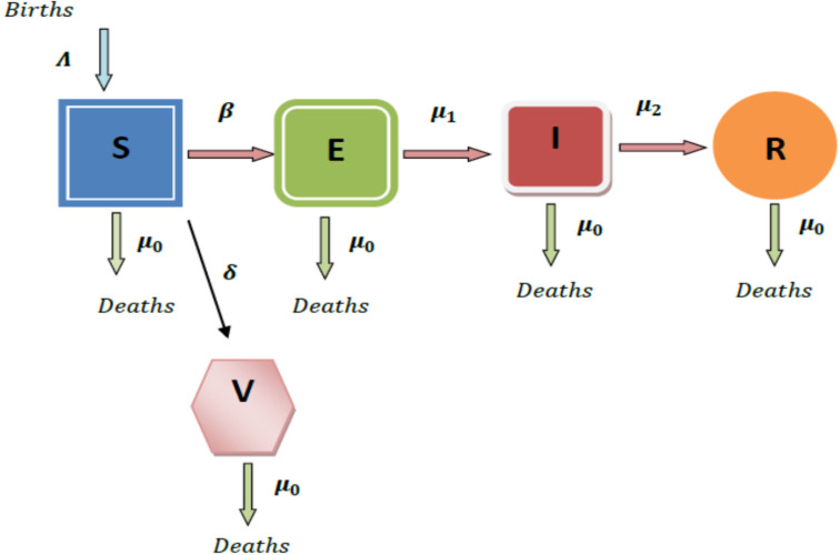
Fig. 1 depicts a flow diagram of the proposed $\mathit{SEIRV}$ model with vaccination.

Fig. 1.

Diagrammatic representation of the $\mathit{SEIRV}$ model.

The Caputo fractional derivative[41], [42], [43], [44], [45] of order $0<\nu \le 1$ is defined as

Definition 1

A function $h:{\mathbb{R}}^{+}\to \mathbb{R}$ with fractional order $0<\nu \le 1$, is defined as

$${}^C{I}_t^{\nu }\left(h\left(t\right)\right)=\frac{1}{\Gamma \left(\nu \right)}{\int }_0^t{(t-p)}^{\nu -1}h\left(p\right)dp,$$ (2.2)

here the Gamma function is denoted by $\Gamma \left(\right)$.

Definition 2

The Caputo derivative of order $0<\nu \le 1$, is defined as

$${}^C{I}_t^{\nu }\left(h\left(t\right)\right)=I^{n-\nu }{D}_t^{\nu }\left(h\left(t\right)\right)=\frac{1}{\Gamma \left(n-\nu \right)}{\int }_0^t{(t-p)}^{n-\nu -1}\frac{d^n}{d{p}^n}h\left(p\right)dp,$$ (2.3)

where $n-1<\nu <n$.

Definition 3

Let $h\in C\left[a,b\right],a<b$. The fractional derivative in Caputo sense or order $0<\nu \le 1$ is defined as

$${}^C{D}_t^{\nu }\left(h\left(t\right)\right)=\frac{M\left(\nu \right)}{(1-\nu )}{\int }_a^t{h}^{\prime }\left(p\right)exp\left(\text{–}\frac{\nu (t-p)}{1-\nu }\right)dp,$$ (2.4)

where the normalization function is denoted by $M\left(\nu \right)$ with $M\left(0\right)=M\left(1\right)=1$.

Definition 4

The Laplace transform for the fractional operator of order $0<\nu \le 1$ is defined as

$$L\left({}^C{D}_t^{\nu }\right)\left(h\left(t\right)\right)=p^{\nu }L\left(h\left(t\right)\right)-\sum _{i=0}^{k-1}{p}^{\nu -i-1}{h}^{\left(i\right)}\left(0\right),k-1<\nu \le k\in \mathbb{N}.$$ (2.5)

Definition 5

One-parametric and two-parametric Mittag-Leffler functions are described as follows: $E_{a_1}\left(p\right)={\sum }_{i=0}^{\infty }\frac{p^i}{\Gamma \left(a_{1}i+1\right)}$ and $E_{a_1,a_2}\left(p\right)={\sum }_{i=0}^{\infty }\frac{p^i}{\Gamma \left(a_{1}i+a_2\right)}$ where $a_1,a_2\in {\mathbb{R}}^{+}$.

Definition 6

For $a_1,a_2\in {\mathbb{R}}^{+}$ and $A\in {ℂ}^{n\times n}$ where $ℂ$ denotes complex plane, then

$$L\left\{t^{a_2-1}{E}_{a_1,a_2}\left(A{t}^{a_1}\right)\right\}=\frac{p^{a_1-a_2}}{p^{a_1}-A},\text{where}{E}_{a_1,a_2}:\text{Mittag-Leffler function}.$$ (2.6)

Lemma 1

Consider the following fractional order system:

$${}^C{D}_t^{\nu }\left(Y\left(t\right)\right)=\Phi \left(Y\right),Y_{t_0}=\left({y_{t_0}}^1,{y_{t_0}}^2,\dots ,{y_{t_0}}^n\right),{y_{t_0}}^j,j=1,2,\dots ,n$$

with $0<\nu <1,Y\left(t\right)=(y^1\left(t\right),y^2\left(t\right),\dots ,y^n\left(t\right))$ and $\Phi \left(Y\right):\left[t_0,\infty \right]\to {\mathbb{R}}^{n\times n}$ . For $\Phi \left(Y\right)=0$ , we get all the equilibrium points. These equilibrium points are locally asymptotically stable iff each eigen value ${\lambda }_j$ of the Jacobian matrix $J\left(Y\right)=\frac{\partial ({\Phi }_1,{\Phi }_2,\dots ,{\Phi }_n)}{\partial (y^1,y^2,\dots ,y^n)}$ calculated at the equilibrium points satisfies $|arg\left({\lambda }_j\right)|>\frac{\nu \pi }{2}$ .

Lemma 2

Let $h\left(t\right)\in {\mathbb{R}}^{+}$ be a differentiable function. Then, for any $t>0$ ,

$${}^C{D}_t^{\nu }\left[h\left(t\right)-h^{\ast }-h^{\ast }ln\frac{h\left(t\right)}{h^{\ast }}\right]\le \left(1-\frac{h^{\ast }}{h\left(t\right)}\right){}^C{D}_t^{\nu }\left(h\left(t\right)\right),h^{\ast }\in {\mathbb{R}}^{+},\forall \nu \in \left(0,1\right).$$

The integral order $\mathit{SEIRV}$ model ^{46 , 47} with vaccination as a dynamical variable is as follows:

$${\mathrm{D}}_{\mathrm{t}}\mathrm{S}\left(\mathrm{t}\right)=\Lambda -\beta S\left(t\right)I\left(t\right)-{\mu }_{0}S\left(t\right)-\delta S\left(t\right)$$

$${\mathrm{D}}_{\mathrm{t}}\mathrm{E}\left(\mathrm{t}\right)=\beta S\left(t\right)I\left(t\right)-({\mu }_0+{\mu }_1)E\left(t\right),$$ (2.7)

$${\mathrm{D}}_{\mathrm{t}}\mathrm{I}\left(\mathrm{t}\right)={\mu }_{1}E\left(t\right)-({\mu }_0+{\mu }_2)I\left(t\right)$$

$${\mathrm{D}}_{\mathrm{t}}\mathrm{R}\left(\mathrm{t}\right)={\mu }_{2}I\left(t\right)-{\mu }_{0}R\left(t\right)$$

$${\mathrm{D}}_{\mathrm{t}}\mathrm{V}\left(\mathrm{t}\right)=\delta S\left(t\right)-{\mu }_{0}V\left(t\right)$$

where

$\Lambda$ : birth rate of $S$ ,

$\beta$ : infection rate of $S$ ,

${\mu }_0$ : mortality rate of $I$ ,

$\delta$ : vaccination rate,

${\mu }_1$ : progression rate from $E$ to $I$ ,

${\mu }_2$ : recovery rate of $I$ .

In this presentation, we analyze the $\mathit{SEIRV}$ model with time delay using Caputo operator of order $0<\nu \le 1$.

$${}^C{D}_t^{\nu }S\left(t\right)={\Lambda }^{\nu }-{\beta }^{\nu }S\left(t\right)I\left(t\right)-{{\mu }_0}^{\nu }S\left(t\right)-{\delta }^{\nu }R\left(t\right),$$

$${}^C{D}_t^{\nu }E\left(t\right)={\beta }^{\nu }S\left(t\right)I\left(t\right)-({{\mu }_0}^{\nu }+{{\mu }_1}^{\nu })E\left(t\right),$$ (2.8)

$${}^C{D}_t^{\nu }I\left(t\right)={{\mu }_1}^{\nu }E\left(t\right)-{{\mu }_0}^{\nu }I\left(t\right)-{{\mu }_2}^{\nu }I\left(t\right),$$

$${}^C{D}_t^{\nu }R\left(t\right)={{\mu }_2}^{\nu }I\left(t\right)-{{\mu }_0}^{\nu }R\left(t\right),$$

$${}^C{D}_t^{\nu }\mathrm{V}\left(\mathrm{t}\right)={\delta }^{\nu }S\left(t\right)-{{\mu }_0}^{\nu }V\left(t\right).$$

The time dimension of the system (2.8) is confirmed to be valid, even though both sides have dimension ${\left(time\right)}^{-\nu }$. Let $t_0=0$ and ignore the super script $\nu$ and the system becomes:

$${}^C{D}_t^{\nu }\mathrm{S}\left(\mathrm{t}\right)=\Lambda -\beta S\left(t\right)I\left(t\right)-{\mu }_{0}S\left(t\right)-\delta S\left(t\right),$$

$${}^C{D}_t^{\nu }\mathrm{E}\left(\mathrm{t}\right)=\beta S\left(t\right)I\left(t\right)-({\mu }_0+{\mu }_1)E\left(t\right),$$ (2.9)

$${}^C{D}_t^{\nu }\mathrm{I}\left(\mathrm{t}\right)={\mu }_{1}E\left(t\right)-{\mu }_{0}I\left(t\right)-{\mu }_{2}I(t-{\eta }_1),$$

$${}^C{D}_t^{\nu }\mathrm{R}\left(\mathrm{t}\right)={\mu }_{2}I(t-{\eta }_1)-{\mu }_{0}R\left(t\right),$$

$${}^C{D}_t^{\nu }\mathrm{V}\left(\mathrm{t}\right)=\delta S\left(t\right)-{\mu }_{0}V\left(t\right),$$

where ${\eta }_1$ is the time delay describing the period of cure the infected individuals.

The initial conditions are

$$S\left(\phi \right)={\psi }_1\left(\phi \right),E\left(\phi \right)={\psi }_2\left(\phi \right),I\left(\phi \right)={\psi }_3\left(\phi \right),R\left(\phi \right)={\psi }_4\left(\phi \right),V\left(\phi \right)={\psi }_5\left(\phi \right),\left(-{\eta }_1\le \phi \le 0\right),$$ (2.10)

where $\psi$ =${\left({\psi }_1,{\psi }_2,{\psi }_3,{\psi }_4,{\psi }_5\right)}^T\in B$, such that ${\psi }_i\left(\phi \right)\ge 0,i=1,2,3,4,5$. Where $\mathrm{B}$ denotes the Banach space of continuous mapping from the interval $[-{\eta }_1,0]$ to ${\mathbb{R}}^5$. We presume, by biological meaning, that ${\psi }_i\left(\phi \right)>0$ for $i=1,2,3,4,5$.

Non-negativity and boundedness

Theorem 2.1

The closed region $\Omega =\{(S,E,I,R,V)\in {\mathbb{R}}^5:0<N\le \frac{\Lambda }{{\mu }_0}\}$ is non-negative invariant of system (2.9) for all $t\ge 0$ .

Proof

We have

$${}^C{D}_t^{\nu }(S+E+I+R+V)\left(t\right)=\lambda -{\mu }_0(S+E+I+R)\left(t\right).$$

• •
  $${}^C{D}_t^{\nu }N\left(t\right)=\lambda -{\mu }_{0}N\left(t\right)$$
• •
  $${}^C{D}_t^{\nu }N\left(t\right)+{\mu }_{0}N\left(t\right)=\lambda .$$ (2.11)

  Applying Laplace transforms, we get

  $$p^{\nu }L\left(N\left(t\right)\right)-p^{\nu -1}N\left(0\right)+{\mu }_{0}L\left(N\left(t\right)\right)=\frac{\lambda }{p}$$
• •
  $$L\left(N\left(t\right)\right)\left(p^{\nu +1}+{\mu }_0\right)=p^{\nu }N\left(0\right)+\lambda$$
• •
  $$L\left(N\left(t\right)\right)=\frac{p^{\nu }N\left(0\right)+\lambda }{p^{\nu +1}+{\mu }_0}=\frac{p^{\nu }N\left(0\right)}{p^{\nu +1}+{\mu }_0}+\frac{\lambda }{p^{\nu +1}+{\mu }_0}.$$ (2.12)

Taking inverse Laplace transform, we have

$$N\left(t\right)=N\left(0\right)E_{\nu ,1}\left(-{\mu }_0{t}^{\nu }\right)+\lambda t^{\nu }{E}_{\nu ,\nu +1}\left(-{\mu }_0{t}^{\nu }\right).$$ (2.13)

According to Mittag-Leffler function,

$$E_{c,d}\left(z\right)=z{E}_{c,c+d}\left(z\right)+\frac{1}{\Gamma \left(d\right)}$$

Hence,

$$N\left(t\right)=\left(N\left(0\right)-\frac{\lambda }{{\delta }_0}\right)E_{\nu ,1}\left(-{\mu }_0{t}^{\nu }\right)+\frac{\lambda }{{\mu }_0}$$

Thus

$$\underset{t\to \infty }{lim}SupN\left(t\right)\le \frac{\lambda }{{\mu }_0}.$$ (2.14)

And hence the model (2.9) is bounded above by $\frac{\lambda }{{\mu }_0}$.

Thus $S,E,I,R$, and $V$ are all non-negative, and the model (2.9) is non-negative invariant.

Basic reproduction number

The basic reproduction number ${\mathfrak{R}}_0$ provides the number of secondary cases induced by single susceptible individual.

Using next generation matrix method,^{48 , 49} ${\mathfrak{R}}_0$ can be determined from the maximum eigen value of $\mathcal{F}{V}^{-1}$ where,

$$\mathcal{F}=\left[\begin{array}{cc}\hfill 0\hfill & \hfill \frac{\beta \Lambda }{{\mu }_0+\delta }\hfill \\ \hfill 0\hfill & \hfill 0\hfill \end{array}\right]\text{and}V=\left[\begin{array}{cc}\hfill {\mu }_0+{\mu }_1\hfill & \hfill 0\hfill \\ \hfill -{\mu }_1\hfill & \hfill {\mu }_0+{\mu }_2\hfill \end{array}\right].$$

Therefore, the reproduction number

$${\mathfrak{R}}_0=\frac{\beta \Lambda {\mu }_1}{\left({\mu }_0+\delta \right)\left({\mu }_0+{\mu }_1\right)({\mu }_0+{\mu }_2)}.$$ (2.15)

3. Stability analysis

The disease-free equilibrium points $E_0$ and the epidemic equilibrium point $E_1$ of are obtained from

$${}^C{D}_t^{\nu }S\left(t\right)={}^C{D}_t^{\nu }E\left(t\right)={}^C{D}_t^{\nu }I\left(t\right)={}^C{D}_t^{\nu }R\left(t\right)={}^C{D}_t^{\nu }V\left(t\right)=0.$$ (3.1)

We have $E_0=\frac{\Lambda }{{\mu }_0+\delta },0,0,0,\frac{\Lambda \delta }{{\mu }_0({\mu }_0+\delta )}$) and $E_1=(S^{\ast },E^{\ast },I^{\ast },R^{\ast },V^{\ast })$,

where $S^{\ast }=\frac{\left({\mu }_0+{\mu }_1\right)({\mu }_0+{\mu }_2)}{\beta {\mu }_1}$, $E^{\ast }=\frac{({\mu }_0+{\mu }_2)}{{\mu }_1}{I}^{\ast }$, $I^{\ast }=\frac{\Lambda {\mu }_1}{\left({\mu }_0+{\mu }_1\right)({\mu }_0+{\mu }_2)}-\frac{{\mu }_0+\delta }{\beta }$,

$R^{\ast }=\frac{{\mu }_2}{{\mu }_0}{I}^{\ast }$, $V^{\ast }=\frac{\left({\mu }_0+{\mu }_1\right)({\mu }_0+{\mu }_2)\delta }{\beta {\mu }_0{\mu }_1}$.

Now we consider the community matrix of the model (2.9) at $E_0$ is given by

$$J_0=P+Q{e}^{-\lambda {\eta }_1},$$

where

$$P=\left[\begin{array}{ccccc}\hfill P_{11}\hfill & \hfill 0\hfill & \hfill P_{13}\hfill & \hfill 0\hfill & \hfill 0\hfill \\ \hfill 0\hfill & \hfill P_{22}\hfill & \hfill P_{23}\hfill & \hfill 0\hfill & \hfill 0\hfill \\ \hfill 0\hfill & \hfill P_{32}\hfill & \hfill P_{33}\hfill & \hfill 0\hfill & \hfill 0\hfill \\ \hfill 0\hfill & \hfill 0\hfill & \hfill 0\hfill & \hfill P_{44}\hfill & \hfill 0\hfill \\ \hfill P_{51}\hfill & \hfill 0\hfill & \hfill 0\hfill & \hfill 0\hfill & \hfill P_{55}\hfill \end{array}\right],Q=\left[\begin{array}{ccccc}\hfill 0\hfill & \hfill 0\hfill & \hfill 0\hfill & \hfill 0\hfill & \hfill 0\hfill \\ \hfill 0\hfill & \hfill 0\hfill & \hfill 0\hfill & \hfill 0\hfill & \hfill 0\hfill \\ \hfill 0\hfill & \hfill 0\hfill & \hfill Q_{33}\hfill & \hfill 0\hfill & \hfill 0\hfill \\ \hfill 0\hfill & \hfill 0\hfill & \hfill Q_{43}\hfill & \hfill 0\hfill & \hfill 0\hfill \\ \hfill 0\hfill & \hfill 0\hfill & \hfill 0\hfill & \hfill 0\hfill & \hfill 0\hfill \end{array}\right],$$

with $P_{11}=-(\delta +{\mu }_0)$, $P_{13}=-\beta S_0$, $P_{22}=-({\mu }_1+{\mu }_0)$, $P_{23}=\beta S_0,P_{32}={\mu }_1$, $P_{33}=-{\mu }_0,P_{44}=-{\mu }_0,P_{51}=\delta ,P_{55}=-{\mu }_0,Q_{33}=-{\mu }_2,Q_{43}={\mu }_2$.

Theorem 3.1

When ${\mathfrak{R}}_0$ < 1, the equilibrium point $E_0$ of the model (2.9) is locally asymptotically stable, and when ${\mathfrak{R}}_0>1$ , it is unstable in the absence of time delay.

Proof

The characteristic equation of $J_0$ is given by determinant $\left(P+Q-\lambda I_5\right)=0$.

The roots of the characteristic equation are $-{\mu }_0$, $-{\mu }_0$, $-(\delta +{\mu }_0)$ and ${\lambda }^2-\lambda \left(P_{22}+P_{33}+Q_{33}\right)+\left(P_{22}{P}_{33}+P_{22}{Q}_{33}-P_{23}{P}_{32}\right)=0$.

The roots are negative if $\left(P_{22}+P_{33}+Q_{33}\right)<0$ and $\left(P_{22}{P}_{33}+P_{22}{Q}_{33}-P_{23}{P}_{32}\right)>0$, using Routh–Hurwitz Criterion.

Now $\left(P_{22}{P}_{33}+P_{22}{Q}_{33}-P_{23}{P}_{32}\right)>0$

$$=>\left({\mu }_1+{\mu }_0\right)\left({\mu }_0+{\mu }_2\right)-\frac{\beta \Lambda {\mu }_1}{\left({\mu }_0+\delta \right)}>0$$

$$=>{\mathfrak{R}}_0<1$$

Therefore the point $E_0$ is locally asymptotically stable or unstable according as ${\mathfrak{R}}_0<1$or ${\mathfrak{R}}_0>1$.

Theorem 3.2

The equilibrium point $E_0$ of the model (2.9) is locally asymptotically stable when ${\eta }_1\in [0,{{\eta }_1}^{\ast }]$ , ${{\eta }_1}^{\ast }=\frac{1}{k}si{n}^{-1}\left(\frac{vx+uy}{x^2+y^2}\right)$ .

Proof

The characteristic equation of $J_0$ is given by determinant $\left(P+Q{e}^{-\lambda {\eta }_1}-\lambda I_5\right)=0$.

Now

$$({\lambda }^5+P_4{\lambda }^4+P_3{\lambda }^3+P_2{\lambda }^2+P_1\lambda +P_0)+\left(Q_4{\lambda }^4+Q_3{\lambda }^3+Q_2{\lambda }^2+Q_1\lambda \right)e^{-\lambda {\eta }_1}=0$$ (3.2)

Where

$$P_4=-\left(P_{11}+P_{22}+P_{33}+P_{44}+P_{55}\right),$$

$$P_3=\left(P_{11}+P_{44}+P_{55}\right)\left(P_{22}+P_{33}\right)\left(P_{11}{P}_{44}+P_{11}{P}_{55}+P_{44}{P}_{55}\right)-(P_{22}{P}_{33}-P_{23}{P}_{32}),$$

$$P_2=\left[-P_{11}{P}_{44}{P}_{55}-\left(P_{11}{P}_{44}+P_{11}{P}_{55}+P_{44}{P}_{55}\right)\left(P_{22}+P_{33}\right)\right)-\left(\left(P_{11}+P_{44}+P_{55}\right)\left(P_{22}{P}_{33}-P_{23}{P}_{32}\right)\right],$$

$$P_1=[P_{11}{P}_{44}{P}_{55}\left(P_{22}+P_{33}\right)+(P_{11}{P}_{44}+P_{11}{P}_{55}+P_{44}{P}_{55})(P_{22}{P}_{33}-P_{23}{P}_{32})],$$

$$P_0=-P_{11}{P}_{44}{P}_{55}\left(P_{22}{P}_{33}-P_{23}{P}_{32}\right),$$

$$Q_4=-Q_{33},$$

$$Q_3=Q_{33}(P_{11}+P_{44}+P_{55}),$$

$$Q_2=-Q_{33}\left(P_{11}{P}_{44}+P_{11}{P}_{55}+P_{44}{P}_{55}\right),$$

$$Q_1=Q_{33}\left(P_{11}{P}_{44}{P}_{55}\right).$$

Let $\lambda =ik$ be a root of the Eq. (3.2), then we have

$$xcos\left(k{\eta }_1\right)+ysin\left(k{\eta }_1\right)=u,xsin\left(k{\eta }_1\right)-ycos\left(k{\eta }_1\right)=v,$$ (3.3)

where

$$x=Q_2{k}^2-Q_4{k}^4,y=Q_3{k}^3-Q_{1}k,u=P_4{k}^4-P_2{k}^2+P_0,v=k^5+P_3{k}^3-P_{1}k$$

We find that

$$x^2+y^2=u^2+v^2=>k^{10}+R_4{k}^8+R_3{k}^6+R_2{k}^4+R_1{k}^2+R_0=0,$$ (3.4)

where

$$R_4=2P_3+{P_4}^2-{Q_4}^2,R_3={P_3}^2-2P_1-2P_4{P}_2-{Q_3}^2+2Q_2{Q}_4,$$

$$R_2=-2P_1{P}_3+{P_2}^2+2P_0{P}_4+2Q_1{Q}_3-{Q_2}^2,$$

$$R_1={P_1}^2-2P_0{P}_2-{Q_1}^2,R_0={P_0}^2.$$

Putting $k^2=t$ in Eq. (3.4), then we have

$$t^5+R_4{t}^4+R_3{t}^3+R_2{t}^2+R_{1}t+R_0=0.$$ (3.5)

If ${t_1}^{\ast }$ is a positive root in Eq. (3.5), then $k=\sqrt{{t_1}^{\ast }}$ is a positive root in Eq. (3.4). Eliminating $cos\left(k{\eta }_1\right)$ from the Eq. (3.3), we obtain

$${{\eta }_1}^{\ast }=\frac{1}{k}si{n}^{-1}\left(\frac{vx+uy}{x^2+y^2}\right)$$

Theorem 3.3

When ${\mathfrak{R}}_0$ < 1, the equilibrium point $E_0$ of the model (2.9) is globally asymptotically stable, and unstable when ${\mathfrak{R}}_0>1$ for any positive ${\eta }_1$ .

Proof

Consider the suitable Lyapunov function:

$$\mathcal{F}\left(\mathrm{t}\right)={\mathcal{F}}_1+{\mathcal{F}}_2$$

where,

$${\mathcal{F}}_1=\left({\mu }_1\right)\mathrm{E}\left(\mathrm{t}\right)+\left({\mu }_0+{\mu }_1\right)\mathrm{I}\left(\mathrm{t}\right)\text{ and}{\mathcal{F}}_2=-{\int }_{\mathrm{t}-{\eta }_1}^{\mathrm{t}}\mathrm{I}\left(\mathrm{z}\right)\mathrm{dz}$$

Taking fractional derivative, we get

$${}^C{D}_t^{\nu }\mathcal{F}\left(t\right)={}^C{D}_t^{\nu }{\mathcal{F}}_1\left(t\right)+{}^C{D}_t^{\nu }{\mathcal{F}}_2\left(t\right)$$

From (2.5) we get,

$${}^C{D}_t^{\nu }\mathcal{F}\left(\mathrm{t}\right)=[{\mu }_1\beta S\left(t\right)I\left(t\right)-\left({\mu }_0+{\mu }_1\right)\left({\mu }_0+{\mu }_2\right)I\left(t\right)].$$ (3.6)

Now,

$${}^C{D}_t^{\nu }\mathcal{F}\left(\mathrm{t}\right)=[\beta S{\mu }_1-\left({\mu }_0+{\mu }_1\right)\left({\mu }_0+{\mu }_2\right)]I$$

Since $S=\frac{\Lambda }{{\mu }_0+\delta }$, it follows that

$${}^C{D}_t^{\nu }\mathcal{F}\left(t\right)=I\left[\left({\mu }_0+{\mu }_1\right)({\mu }_0+{\mu }_2)\right][\frac{\beta \Lambda {\mu }_1}{\left({\mu }_0+\delta \right)\left({\mu }_0+{\mu }_1\right)({\mu }_0+{\mu }_2)}-1]=I\left[\left({\mu }_0+{\mu }_1\right)({\mu }_0+{\mu }_2)\right][{\mathfrak{R}}_0-1].$$

Hence if ${\mathfrak{R}}_0<1$, then ${}^C{D}_t^{\nu }\mathcal{F}\left(\mathrm{t}\right)<0$. As a result of LaSalle’s extension to Lyapunov’s principle,^{50 , 51} $E_0$ is globally asymptotically stable and unstable if ${\mathfrak{R}}_0>1$.

Theorem 3.4

If ${\mathfrak{R}}_0>1$ , the equilibrium point $E_1=(S^{\ast },E^{\ast },I^{\ast },R^{\ast },V^{\ast })$ is locally asymptotically stable when ${\eta }_1=0$ .

Proof

The characteristic equation of the system (2.9) at the epidemic equilibrium $E_1$ is $\left(-{\mu }_0-\lambda \right)\left(-{\mu }_0-\lambda \right)$ (${\lambda }^3+A{\lambda }^2+B\lambda +C)=0$.

where

$$A=-\left(G_{11}+G_{22}+G_{33}+H_{33}\right),$$

$$B=G_{11}\left(G_{22}+G_{33}+H_{33}\right)+\left(G_{22}{G}_{33}-G_{23}{G}_{32}+G_{13}{G}_{21}{G}_{32}\right),$$

$$C=-G_{11}(G_{22}{G}_{33}-G_{23}{G}_{32}+G_{13}{G}_{21}{G}_{32}),$$

with

$$G_{11}=-\beta I^{\ast }-\delta -{\mu }_0,G_{22}=-{\mu }_0-{\mu }_1,G_{33}=-{\mu }_0,H_{33}=-{\mu }_2,G_{13}=-\beta S^{\ast },G_{23}=\beta S^{\ast },G_{32}={\mu }_1,G_{21}=\beta I^{\ast },G_{23}=\beta I^{\ast }.$$

Using Routh–Hurwitz Criterion, the system (2.9) is locally asymptotically stable at $E_1$ as $A>0,C>0,AB>C$.

Theorem 3.5

The epidemic equilibrium $E_1=(S^{\ast },E^{\ast },I^{\ast },R^{\ast },V^{\ast })$ of the system (2.9) is locally asymptotically stable when ${\eta }_1\in [0,{{\eta }_1}^{\ast }]$ , ${{\eta }_1}^{\ast }=\frac{1}{m_{10}}si{n}^{-1}\left(\frac{ad+bc}{a^2+b^2}\right)$ ; system (2.9) undergoes a Hopf bifurcation at $E_1$ when ${\eta }_1={{\eta }_1}^{\ast }$ .

Proof

The characteristic equation of the system (2.9) at the epidemic equilibrium $E_1$ is given by determinant $\left(G+H{e}^{-\lambda {\eta }_1}-\lambda I_5\right)=0$.

Now

$${\lambda }^5+A_4{\lambda }^4+A_3{\lambda }^3+A_2{\lambda }^2+A_1\lambda +A_0+\left(B_4{\lambda }^4+B_3{\lambda }^3+B_2{\lambda }^2+B_1\lambda +B_0\right)e^{-\lambda {\eta }_1}=0.$$ (3.7)

where

$$A_4=-\left(G_{11}+G_{22}+G_{33}+G_{44}+G_{55}\right),$$

$$A_3=(G_{11}{G}_{22}-G_{23}{G}_{32}+G_{11}{G}_{33}+G_{22}{G}_{33}+G_{11}{G}_{44}+G_{22}{G}_{44}+G_{33}{G}_{44}+G_{11}{G}_{55}+G_{22}{G}_{55}+G_{33}{G}_{55}),$$

$$A_2=\left[-G_{13}{G}_{21}{G}_{32}+G_{11}{G}_{23}{G}_{32}-G_{11}{G}_{22}{G}_{33}-G_{11}{G}_{22}{G}_{44}+G_{23}{G}_{32}{G}_{44}\right)-G_{11}{G}_{33}{G}_{44}-G_{22}{G}_{33}{G}_{44}-G_{11}{G}_{22}{G}_{55}+G_{23}{G}_{32}{G}_{55}-G_{11}{G}_{33}{G}_{55}-G_{22}{G}_{33}{G}_{55}+G_{44}{G}_{55}-G_{11}{G}_{44}{G}_{55}-\left(G_{22}{G}_{44}{G}_{55}-G_{33}{G}_{44}{G}_{55}\right],$$

$$A_1=[G_{13}{G}_{21}{G}_{32}{G}_{44}-G_{11}{G}_{23}{G}_{32}{G}_{44}+G_{11}{G}_{22}{G}_{33}{G}_{44}+G_{13}{G}_{21}{G}_{32}{G}_{55}-G_{11}{G}_{23}{G}_{32}{G}_{55}+G_{11}{G}_{22}{G}_{33}{G}_{55}+G_{11}{G}_{22}{G}_{44}{G}_{55}-G_{23}{G}_{32}{G}_{44}{G}_{55}+G_{11}{G}_{33}{G}_{44}{G}_{55}+G_{22}{G}_{33}{G}_{44}{G}_{55}],$$

$$A_0=-G_{13}{G}_{21}{G}_{32}{G}_{44}{G}_{55}+G_{11}{G}_{23}{G}_{32}{G}_{44}{G}_{55}-G_{11}{G}_{22}{G}_{33}{G}_{44}{G}_{55},$$

$$B_4=-H_{33},$$

$$B_3=G_{11}{H}_{33}+G_{22}{H}_{33}+G_{44}{H}_{33}+G_{55}{H}_{33},$$

$$B_2=-G_{11}{G}_{22}{H}_{33}-G_{11}{G}_{44}{H}_{33}-G_{22}{G}_{44}{H}_{33}-G_{11}{G}_{55}{H}_{33}-G_{22}{G}_{55}{H}_{33}-G_{44}{G}_{55}{H}_{33},$$

$$B_1=G_{11}{G}_{22}{G}_{44}{H}_{33}+G_{11}{G}_{22}{G}_{55}{H}_{33}+G_{11}{G}_{44}{G}_{55}{H}_{33}+G_{22}{G}_{44}{G}_{55}{H}_{33},$$

$$B_0=G_{11}{G}_{22}{G}_{44}{G}_{55}{H}_{33},$$

with $G=\left[\begin{array}{ccccc}\hfill G_{11}\hfill & \hfill 0\hfill & \hfill G_{13}\hfill & \hfill 0\hfill & \hfill 0\hfill \\ \hfill G_{21}\hfill & \hfill G_{22}\hfill & \hfill G_{23}\hfill & \hfill 0\hfill & \hfill 0\hfill \\ \hfill 0\hfill & \hfill G_{32}\hfill & \hfill G_{33}\hfill & \hfill 0\hfill & \hfill 0\hfill \\ \hfill 0\hfill & \hfill 0\hfill & \hfill 0\hfill & \hfill G_{44}\hfill & \hfill 0\hfill \\ \hfill G_{51}\hfill & \hfill 0\hfill & \hfill 0\hfill & \hfill 0\hfill & \hfill G_{55}\hfill \end{array}\right]$, $H=\left[\begin{array}{ccccc}\hfill 0\hfill & \hfill 0\hfill & \hfill 0\hfill & \hfill 0\hfill & \hfill 0\hfill \\ \hfill 0\hfill & \hfill 0\hfill & \hfill 0\hfill & \hfill 0\hfill & \hfill 0\hfill \\ \hfill 0\hfill & \hfill 0\hfill & \hfill H_{33}\hfill & \hfill 0\hfill & \hfill 0\hfill \\ \hfill 0\hfill & \hfill 0\hfill & \hfill H_{43}\hfill & \hfill 0\hfill & \hfill 0\hfill \\ \hfill 0\hfill & \hfill 0\hfill & \hfill 0\hfill & \hfill 0\hfill & \hfill 0\hfill \end{array}\right]$,

where $G_{11}=-(\beta I^{\ast }+\delta +{\mu }_0)$, $G_{13}=-\beta S^{\ast }$, $G_{21}=\beta I^{\ast },G_{22}=-({\mu }_1+{\mu }_0)$, $G_{23}=\beta S^{\ast },G_{32}={\mu }_1$, $G_{33}=-{\mu }_0,G_{44}=-{\mu }_0,G_{51}=\delta ,G_{55}=-{\mu }_0,H_{33}=-{\mu }_2,H_{43}={\mu }_2$.

If we consider $\lambda$ $=i{m}_1$ to be a root of the Eq. (3.7), we get

$$acos\left(m_1{\eta }_1\right)+bsin\left(m_1{\eta }_1\right)=c,asin\left(m_1{\eta }_1\right)-bcos\left(m_1{\eta }_1\right)=d,$$ (3.8)

where

$$a=B_2{m_1}^2-B_4{m_1}^4-B_0,b=B_3{m_1}^3-B_1{m}_1,c=A_4{m_1}^4-A_2{m_1}^2+A_0,d={m_1}^5+A_3{m_1}^3-A_1{m}_1$$

Now we have

$$a^2+b^2=c^2+d^2=>{m_1}^{10}+L_4{m_1}^8+L_3{m_1}^6+L_2{m_1}^4+L_1{m_1}^2+L_0=0,$$ (3.9)

where

$$L_4=2A_3+{A_4}^2-{B_4}^2,L_3={A_3}^2-2A_1-2A_4{A}_2-{B_3}^2+2B_2{B}_4,$$

$$L_2=-2A_1{A}_3+{A_2}^2+2A_0{A}_4+2B_1{B}_3-{B_2}^2+2B_0{B}_4,$$

$$L_1={A_1}^2-2A_0{A}_2-{B_1}^2-2B_0{B}_2,$$

$$L_0={A_0}^2-{B_0}^2.$$

Put ${m_1}^2=j$ in Eq. (3.9), then we have

$$j^5+L_4{j}^4+L_3{j}^3+L_2{j}^2+L_{1}j+L_0=0.$$ (3.10)

Now consider that

Case-1: If $j_0$ is a positive root in Eq. (3.10), then $m_{10}=\sqrt{j_0}$ is a positive root in Eq. (3.9).

Eliminating $cos\left(m_1{\eta }_1\right)$ from (3.8) and substituting $m_1=m_{10}$, where $m_{10}$ is a positive root of Eq. (3.9), we have

$${{\eta }_1}^{\ast }=\frac{1}{m_{10}}si{n}^{-1}\left(\frac{ad+bc}{a^2+b^2}\right)$$

Now, by differentiating Eq. (3.7) with regard to ${\eta }_1$ and simplifying with $\lambda$ $=i{m}_{10}$, we get

$$\text{Re}{{\left[\frac{d\lambda }{d{\eta }_1}\right]}^{-1}}_{\lambda =i{m}_{10}}=\frac{f_1^{\prime }\left(j_0\right)}{a^2+b^2}$$ (3.11)

Therefore, Re ${{\left[\frac{d\lambda }{d{\eta }_1}\right]}^{-1}}_{\lambda =i{m}_{10}}\ne 0$ if the condition

$f_1^{\prime }\left(j_0\right)=\frac{d{f}_1\left(j\right)}{dj}\ne 0$ at $j=j_0$ holds, where $f_1\left(j\right)=j^5+L_4{j}^4+L_3{j}^3+L_2{j}^2+L_{1}j+L_0$.

Thus, according to the Hopf bifurcation theorem,⁵² we obtain the result of Theorem 3.5 if Case-1 hold.

Theorem 3.6

The epidemic equilibrium $E_1$ is globally asymptotically stable if ${\mathfrak{R}}_0>1$ .

Proof

Consider the non-linear Lyapunov function:

$$W\left(t\right)=\left(S\left(t\right)-S^{\ast }-S^{\ast }log\frac{S\left(t\right)}{S^{\ast }}\right)+\left(E\left(t\right)-E^{\ast }-E^{\ast }log\frac{E\left(t\right)}{E^{\ast }}\right)+Q\left(I\left(t\right)-I^{\ast }-I^{\ast }log\frac{I\left(t\right)}{I^{\ast }}\right).$$

Using Lemma 2 and taking the fractional derivative of $W\left(t\right)$ with respect to time is,

$${}^C{D}_t^{\nu }W\left(t\right)\le \left(1-\frac{S^{\ast }}{S\left(t\right)}\right){}^C{D}_t^{\nu }S\left(t\right)+\left(1-\frac{E^{\ast }}{E\left(t\right)}\right){}^C{D}_t^{\nu }E\left(t\right)+Q\left(1-\frac{I^{\ast }}{I\left(t\right)}\right){}^C{D}_t^{\nu }\mathrm{I}\left(\mathrm{t}\right).$$ (3.12)

Using system (2.9) we get,

$${}^C{D}_t^{\nu }W\left(t\right)\le \left(\Lambda -\beta S\left(t\right)I\left(t\right)-{\mu }_{0}S\left(t\right)-\delta S\left(t\right)-\frac{S^{\ast }(\Lambda -\beta S\left(t\right)I\left(t\right)-{\mu }_{0}S\left(t\right)-\delta S\left(t\right))}{S\left(t\right)}\right)+\left((\beta S\left(t\right)I\left(t\right)-\left({\mu }_0+{\mu }_1\right)E\left(t\right))-\frac{E^{\ast }(\beta S\left(t\right)I\left(t\right)-\left({\mu }_0+{\mu }_1\right)E\left(t\right))}{E\left(t\right)}\right)+Q\left(({\mu }_{1}E\left(t\right)-{\mu }_{0}I\left(t\right)-{\mu }_{2}I(\mathrm{t}-{\eta }_1))-\frac{I^{\ast }\left({\mu }_{1}E\left(t\right)-{\mu }_{0}I\left(t\right)-{\mu }_{2}I(\mathrm{t}-{\eta }_1)\right)}{I\left(t\right)}\right).$$ (3.13)

We have Eq. (2.9) in steady state,

$$\Lambda =\beta S^{\ast }{I}^{\ast }+{\mu }_0{S}^{\ast }+\delta S^{\ast }.$$ (3.14)

Substituting Eq. (3.14) into (3.13) we have,

$${}^C{D}_t^{\nu }W\left(t\right)\le \left(\beta S^{\ast }{I}^{\ast }+{\mu }_0{S}^{\ast }+\delta S^{\ast }-\beta S\left(t\right)I\left(t\right)-{\mu }_{0}S\left(t\right)-\delta S\left(t\right)\right)-\left(\frac{S^{\ast }(\beta S^{\ast }{I}^{\ast }+{\mu }_0{S}^{\ast }+\delta S^{\ast }-\beta S\left(t\right)I\left(t\right)-{\mu }_{0}S\left(t\right)-\delta S\left(t\right))}{S\left(t\right)}\right)+\left((\beta S\left(t\right)I\left(t\right)-\left({\mu }_0+{\mu }_1\right)E\left(t\right))-\frac{E^{\ast }(\beta S\left(t\right)I\left(t\right)-\left({\mu }_0+{\mu }_1\right)E\left(t\right))}{E\left(t\right)}\right)+Q\left(({\mu }_{1}E\left(t\right)-{\mu }_{0}I\left(t\right)-{\mu }_{2}I(\mathrm{t}-{\eta }_1))\right)\left(-\frac{I^{\ast }\left({\mu }_{1}E\left(t\right)-{\mu }_{0}I\left(t\right)-{\mu }_{2}I(\mathrm{t}-{\eta }_1)\right)}{I\left(t\right)}\right).$$

Further simplification gives,

$${}^C{D}_t^{\nu }W\left(t\right)\le \left(\beta S^{\ast }{I}^{\ast }+{\mu }_0{S}^{\ast }+\delta S^{\ast }-{\mu }_{0}S\left(t\right)-\delta S\left(t\right)\right)-\left(\frac{S^{\ast }(\beta S^{\ast }{I}^{\ast }+{\mu }_0{S}^{\ast }+\delta S^{\ast }-\beta S\left(t\right)I\left(t\right)-{\mu }_{0}S\left(t\right)-\delta S\left(t\right))}{S\left(t\right)}\right)+\left((-\left({\mu }_0+{\mu }_1\right)E\left(t\right))-\frac{E^{\ast }(\beta S\left(t\right)I\left(t\right)-\left({\mu }_0+{\mu }_1\right)E\left(t\right))}{E\left(t\right)}\right)+Q\left(({\mu }_{1}E\left(t\right)-{\mu }_{0}I\left(t\right)-{\mu }_{2}I(\mathrm{t}-{\eta }_1))\right)-\left(\frac{I^{\ast }\left({\mu }_{1}E\left(t\right)-{\mu }_{0}I\left(t\right)-{\mu }_{2}I(\mathrm{t}-{\eta }_1)\right)}{I\left(t\right)}\right).$$ (3.15)

Collecting all infected classes from (3.15) to zero without a single star (*):

$$S^{\ast }\beta I\left(t\right)-\left({\mu }_0+{\mu }_1\right)E\left(t\right)+Q\left({\mu }_{1}E\left(t\right)--{\mu }_{0}I\left(t\right)-{\mu }_{2}I(\mathrm{t}-{\eta }_1)\right)=0.$$ (3.16)

The steady state of equilibrium point (2.9), we get

$$Q=\frac{S^{\ast }\beta }{\left({\mu }_0+{\mu }_2\right)},\left({\mu }_0+{\mu }_1\right)=\frac{I^{\ast }{S}^{\ast }\beta }{E^{\ast }},{\mu }_1=\frac{({\mu }_0+{\mu }_2)I^{\ast }}{E^{\ast }}.$$ (3.17)

Substituting the expression from (3.17) into (3.15) gives:

$${}^C{D}_t^{\nu }W\left(t\right)\le \left(\beta S^{\ast }{I}^{\ast }+{\mu }_0{S}^{\ast }+\delta S^{\ast }-{\mu }_{0}S-\delta S\left(t\right)\right)-\left(\frac{S^{\ast }(\beta S^{\ast }{I}^{\ast }+{\mu }_0{S}^{\ast }-{\mu }_{0}S-\delta S)}{S}\right)+\left(-\frac{E^{\ast }\beta SI}{E}+I^{\ast }{S}^{\ast }\beta \right)+(-\frac{I^{\ast }{S}^{\ast }E\beta I^{\ast }}{I{E}^{\ast }}+\beta S^{\ast }{I}^{\ast }).$$

Using $A.M.\ge G.M.$, we get:

$$(2-\frac{s}{S^{\ast }}-\frac{S^{\ast }}{S})\le 0,(3-\frac{S^{\ast }}{S}-\frac{I^{\ast }E}{I{E}^{\ast }}-\frac{S{E}^{\ast }I}{E})\le 0.$$

Thus

$${}^C{D}_t^{\nu }W\left(t\right)\le 0\text{for}{\mathfrak{R}}_0>1$$

Therefore $E_1$ is globally asymptotically stable, according to LaSalle’s Invariance Principle.⁵¹

4. Adam–Bashforth–Moulton method for the $\mathit{SEIRV}$ model

For fractional order initial value situations, the Adams–Bashforth–Moulton​ approach is the most commonly used numerical technique.

Let

$${}^C{D}_t^{\nu }{L}_j\left(t\right)=g_j(t,L_j\left(t\right),L_j(t-{\eta }_1)),t\in \left[-{\eta }_1,0\right],L_j^r\left(0\right)=L_{j0}^r,$$ (4.1)

$r=0,1,2,\dots ,⌈\nu ⌉$, $j\in \mathbb{N}$

where $L_{j0}^r\in \mathbb{R}$, $\nu >0$ and ${}^C{D}_t^{\nu }$ is same as Volterra integral equation in the Caputo sense.

$$L_j\left(t\right)=\sum _{n=0}^{⌈\nu ⌉-1}{L}_{j0}^r\frac{t^n}{n!}+\frac{1}{\Gamma \left(\nu \right)}{\int }_0^t{(t-u)}^{\nu -1}{g}_j(u,L_j\left(u\right),L_j(u-{\eta }_1))du,j\in \mathbb{N}.$$ (4.2)

Let $h=\frac{T}{\hat{m}},t_n=nh,n=0,1,2,\dots ,\hat{m}$.

Corrector formulae:

$$S_{n+1}=S_0+\frac{h^{\nu }}{\Gamma \left(\nu +2\right)}\left(\Lambda -\beta S_{n+1}^p{I}_{n+1}^p-{\mu }_0{S}_{n+1}^p-\delta S_{n+1}^p\right)+\frac{h^{\nu }}{\Gamma \left(\nu +2\right)}\sum _{j=0}^n{\alpha }_{j,n+1}\left(\Lambda -\beta S_j{I}_j-{\mu }_0{S}_j-\delta S_j\right),$$

$$E_{n+1}=E_0+\frac{h^{\nu }}{\Gamma \left(\nu +2\right)}\left(\beta S_{n+1}^p{I}_{n+1}^p-({\mu }_0+{\mu }_1)E_{n+1}^p\right)+\frac{h^{\nu }}{\Gamma \left(\nu +2\right)}\sum _{j=0}^n{\alpha }_{j,n+1}(\beta S_j{I}_j-({\mu }_0+{\mu }_1)E_j),$$

$$I_{n+1}=I_0+\frac{h^{\nu }}{\Gamma \left(\nu +2\right)}\left({\mu }_1{E}_{n+1}^p-({\mu }_0+{\mu }_2)I_{n+1}^p\right)+\frac{h^{\nu }}{\Gamma \left(\nu +2\right)}\sum _{j=0}^n{\alpha }_{j,n+1}({\mu }_1{E}_j-({\mu }_0+{\mu }_2)I_j),$$

$$R_{n+1}=R_0+\frac{h^{\nu }}{\Gamma \left(\nu +2\right)}\left({\mu }_2{I}_{n+1}^p-{\mu }_0{R}_{n+1}^p\right)+\frac{h^{\nu }}{\Gamma \left(\nu +2\right)}\sum _{j=0}^n{\alpha }_{j,n+1}({\mu }_2{I}_j-{\mu }_0{R}_j),$$

$$V_{n+1}=V_0+\frac{h^{\nu }}{\Gamma \left(\nu +2\right)}\left(\delta S_{n+1}^p-{\mu }_0{V}_{n+1}^p\right)+\frac{h^{\nu }}{\Gamma \left(\nu +2\right)}\sum _{j=0}^n{\alpha }_{j,n+1}(\delta S_j-{\mu }_0{V}_j).$$ (4.3)

Predictor formulae:

$$S_{n+1}^p=S_0+\frac{1}{\Gamma \left(\nu \right)}\sum _{j=0}^n{\Theta }_{j,n+1}\left(\Lambda -\beta S_j{I}_j-{\mu }_0{S}_j-\delta S_j\right),$$

$$E_{n+1}^p=E_0+\frac{1}{\Gamma \left(\nu \right)}\sum _{j=0}^n{\Theta }_{j,n+1}(\beta S_j{I}_j-({\mu }_0+{\mu }_1)E_j),$$ (4.4)

$$I_{n+1}^p=I_0+\frac{1}{\Gamma \left(\nu \right)}\sum _{j=0}^n{\Theta }_{j,n+1}({\mu }_1{E}_j-({\mu }_0+{\mu }_2)I_j),$$

$$R_{n+1}^p=R_0+\frac{1}{\Gamma \left(\nu \right)}\sum _{j=0}^n{\Theta }_{j,n+1}({\mu }_2{I}_j-{\mu }_0{R}_j),$$

$$V_{n+1}^p=V_0+\frac{1}{\Gamma \left(\nu \right)}\sum _{j=0}^n{\Theta }_{j,n+1}(\delta S_j-{\mu }_0{V}_j),$$

where

$${\nu }_{j,n+1}=\left\{\begin{array}{cc}{n}^{\nu +1}-\left(n-\nu \right){(n+1)}^{\nu },\hfill & ifj=0,\hfill \\ {(n-j+2)}^{\nu +1}+{(n-j)}^{\nu +1}-2{(n-j+1)}^{\nu +1},\hfill & if0\le j\le n,\hfill \\ 1,\hfill & ifj=1,\hfill \end{array}\right)$$

and

$${\Theta }_{j,n+1}=\frac{h^{\nu }}{\nu }\left[{(n+1-j)}^{\nu }-{\left(n-j\right)}^{\nu }\right],0\le j\le n.$$

5. Numerical simulation

We have studied and analyzed the dynamical behavior of the solutions of (2.9) using an extensive numerical simulation. In this section, we use MATLAB to analyze the solutions generated by Adams–Bashforth–Moulton scheme. The results of model simulations and the associated findings have been classified as follows:

Case - $\mathbf{I}$

In this case, we analyze the dynamical characteristics of all population for various fractional order with ${\eta }_1=0$.

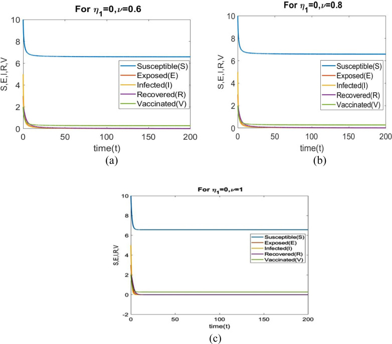
From Figs. 2(a) to 2(c) illustrate that when ${\mathfrak{R}}_0<1$, the number of exposed individuals, infected individuals and recovered individuals drops to zero. So the point $E_0$ is locally asymptotically stable when ${\mathfrak{R}}_0<1$ for different values of $\nu$. Table 1 displays the values of parameters.

Fig. 2.

Time series analysis corresponding to ${\eta }_1=0$ for (a) $\nu =0.6$ (b) $\nu =0.8$ (c) $\nu =1$.

Parameters	Value	Source
$\Lambda$	5	Estimated
$\beta$	0.01	Estimated
${\mu }_0$	0.731	Estimated
$\delta$	0.03	Model to fit
${\mu }_1$	0.015	Estimated
${\mu }_2$	0.5	Estimated
${\mathfrak{R}}_0$	0.0534	Estimated

Case - $\mathbf{II}$

In this case, we analyze the dynamical characteristics of all population for various fractional order with ${\eta }_1=0$, ${\eta }_1=0.5$ and ${\eta }_1=2$.

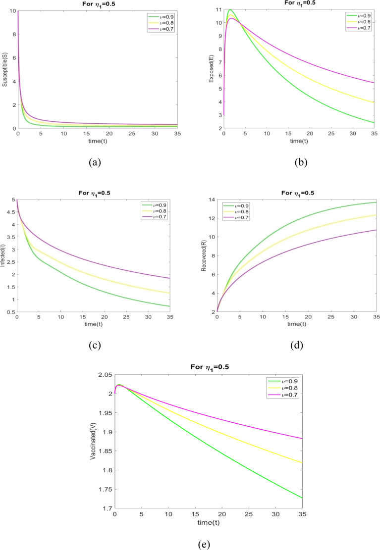
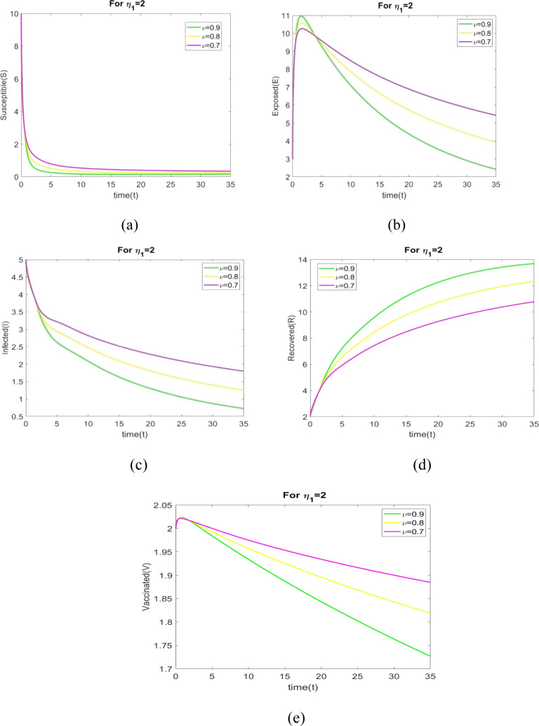
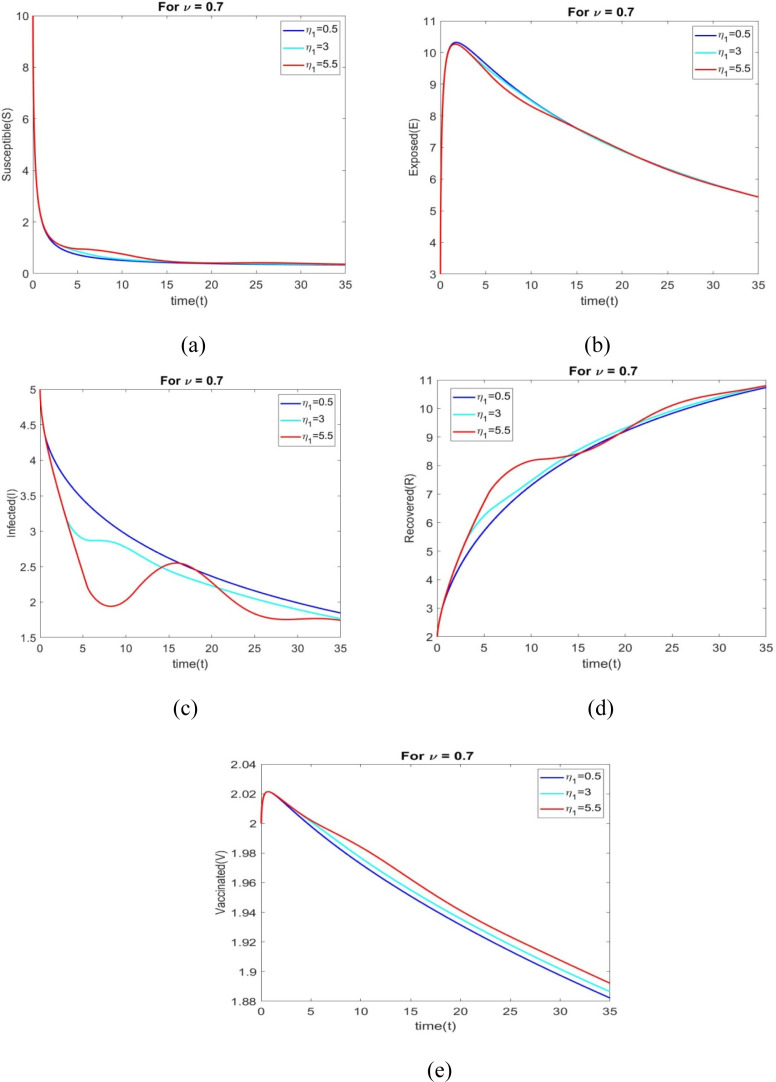
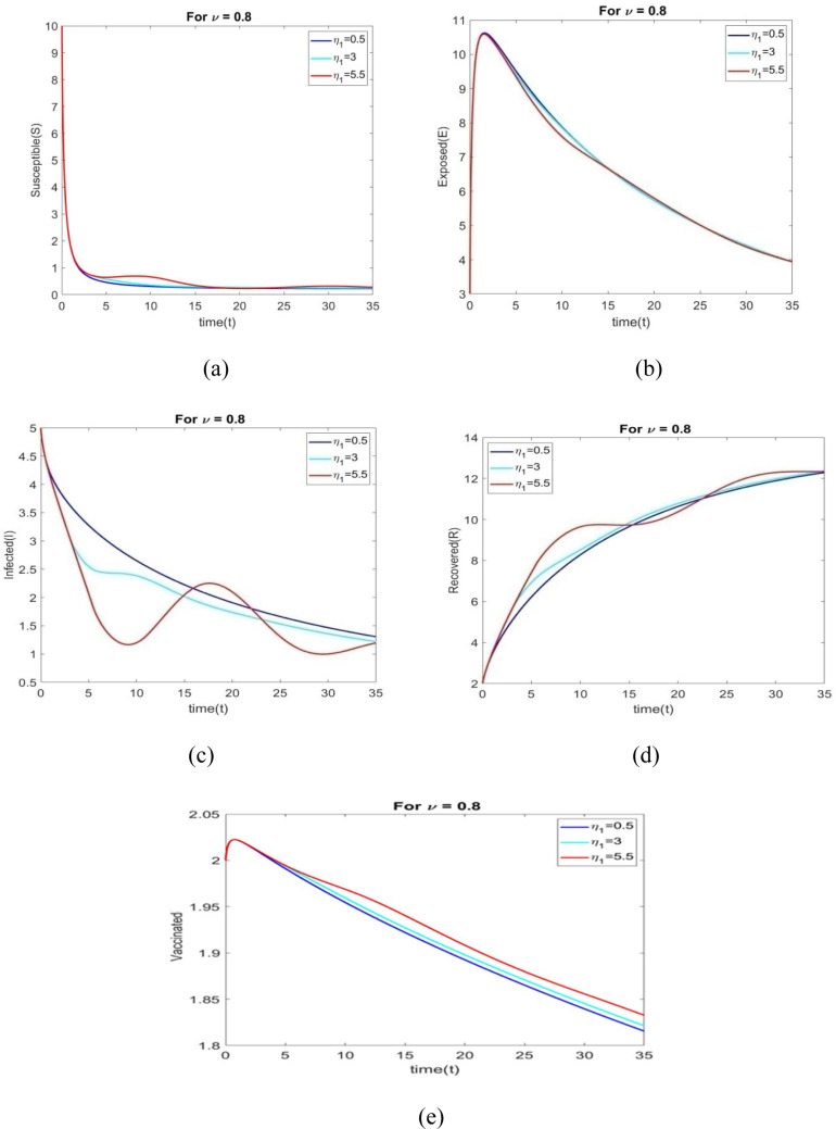
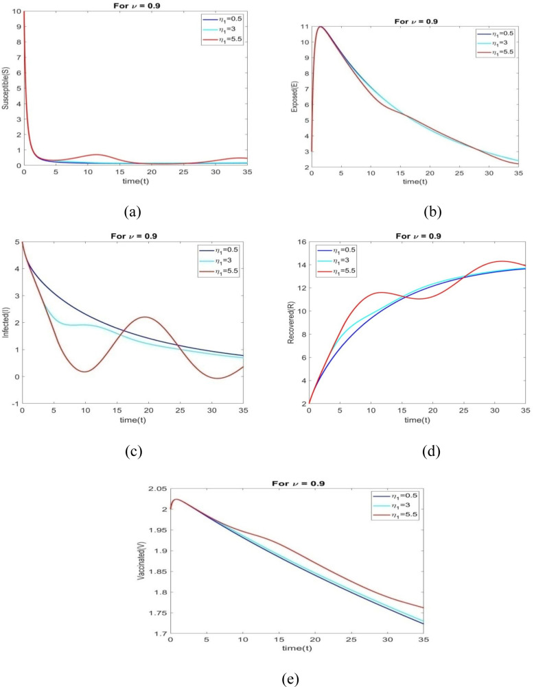
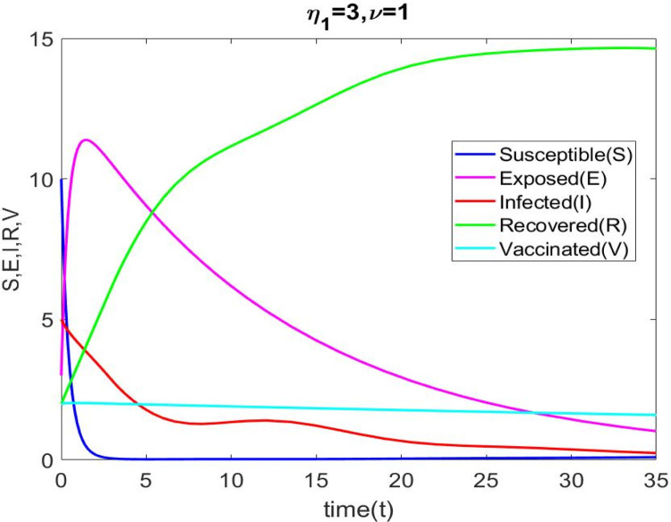
The values of parameters in Table 2 are used to plot the figures in Fig. 3, Fig. 4, Fig. 5, Fig. 6, Fig. 7, Fig. 8, Fig. 9, Fig. 10. The behavior of all individuals with time corresponding to ${\eta }_1=0.5$ for different fractional order $\nu$ is shown in Figs. 3(a) through 3(e). The number of susceptible individuals and infected individuals decreases when $\nu$ increases. The number of recovered individuals increases when $\nu$ increases.

Parameters	Value	Source
$\Lambda$	0.0182	Estimated
$\beta$	0.476	Estimated
${\mu }_0$	0.0073	Estimated
$\delta$	0.01	Model to fit
${\mu }_1$	0.071	53,54
${\mu }_2$	0.286	53,54
${\mathfrak{R}}_0$	1.55	Estimated

Fig. 3.

The behavior of $S,E,I,R$ and $V$ for varied values of $\nu =0.9,0.8,0.7$ with ${\eta }_1=0.5$.

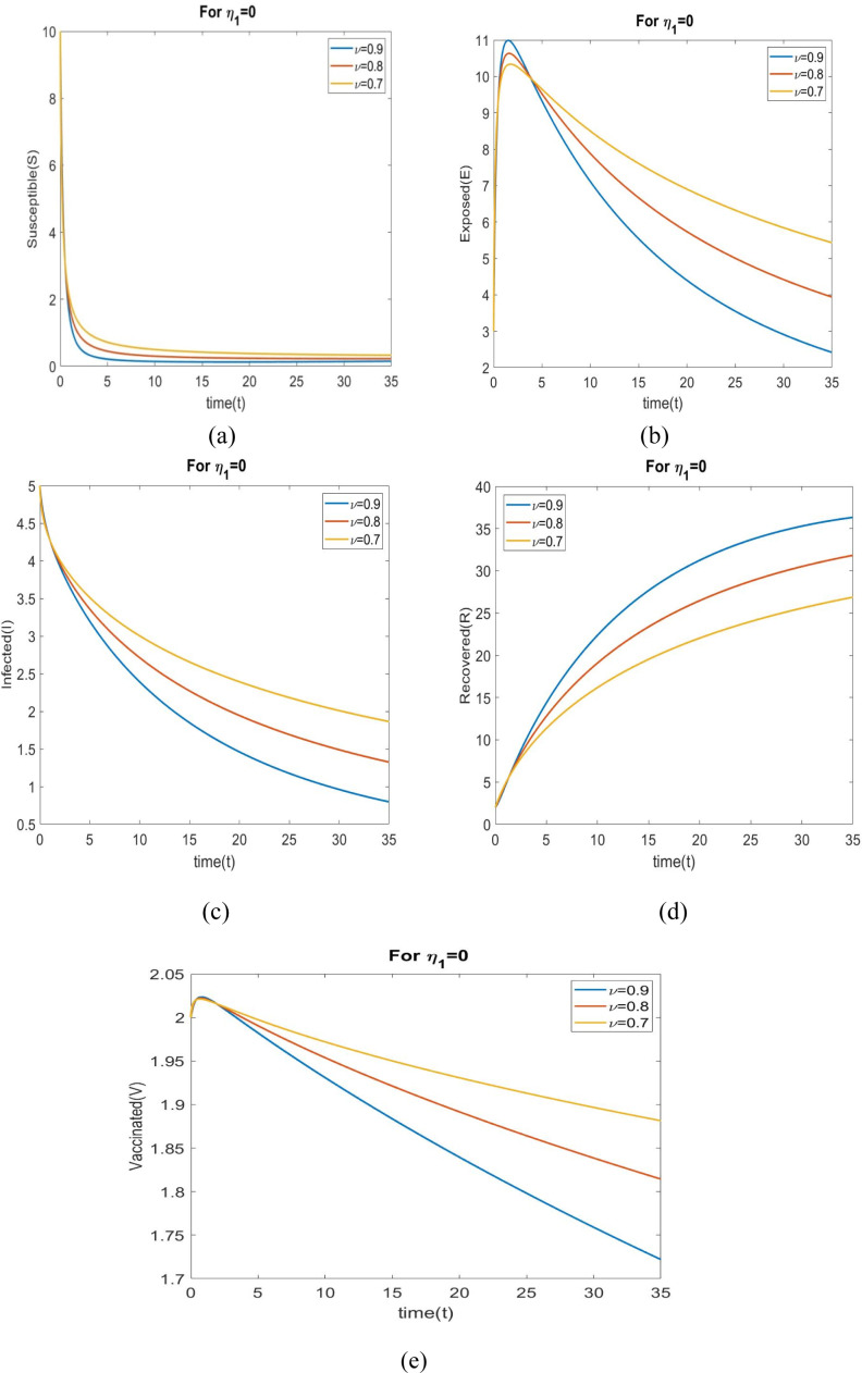
Fig. 4.

The behavior of all individuals for different values of $\nu =0.9,0.8,0.7$ with ${\eta }_1=0$.

Fig. 5.

The behavior of all individuals for values of $\nu =0.9,0.8,0.7$ and ${\eta }_1=2$.

Fig. 6.

Dynamical behavior of all individuals for $\nu =0.7$ and different values of ${\eta }_1=0$.5, 3, 5.5.

Fig. 7.

Dynamical behavior of all individuals for $\nu =0.8$ and different values of ${\eta }_1=0$.5, 3, 5.5.

Fig. 8.

The behavior of all individuals for $\nu =0.9$ and different values of ${\eta }_1=0$.5, 3, 5.5.

Fig. 9.

Time series analysis for ${\eta }_1=3$ and $\nu =1$ of Eq. (2.9).

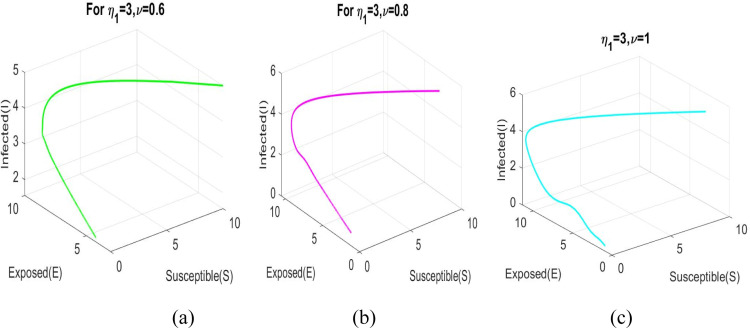
Fig. 10.

Phase diagram of the model (2.9) corresponding to ${\eta }_1=3$ and $\nu =0.6,0.8,1$.

Figs. 4(a) to 4(e) shows the behavior of all individuals with time corresponding to ${\eta }_1=0$ for different fractional order $\nu$. Fig. 4(a) depicts that the number of susceptible individuals increase when $\nu$ changes to 0.9 to 0.7. An increase value of $\nu$ leads to decrease in the exposed rate in the exposed population in Fig. 4(b). We see in Fig. 4(c) that number of infected individuals increase when $\nu$ changes to 0.9 to 0.7. Fig. 4(d) depicts that the number of recovered individuals increase with time when $\nu$ increases.

The behavior of all individuals with time corresponding to ${\eta }_1=2$ for different fractional order $\nu$ is shown in Figs. 5(a) through 5(e). Fig. 5(a) depicts that the number of susceptible individuals increase when $\nu$ increases. We see in Fig. 5(c) that number of infected individuals increase when $\nu$ changes to 0.9 to 0.7. Fig. 5(d) depicts that the number of recovered individuals increase when $\nu$ increases.

The behavior of all individuals with time corresponding to $\nu =0.7$ is shown in Figs. 6(a) through 6(e) for various time delays ${\eta }_1$.

Figs. 7(a) to 7(e) shows the behavior of all individuals with time corresponding to $\nu =0.8$ for different time delays ${\eta }_1$. The number of vaccinated individuals increase when ${\eta }_1$ changes to 0.5 to 5.5.

The performance of all individuals with time corresponding to $\nu =0.9$ is shown in Figs. 8(a) through 8(e) for various time delays ${\eta }_1$.

Case - $\mathbf{III}$

The existence of the Hopf bifurcation of the model system (2.9) with fractional order $\nu =1$ is discussed in this case. The following set of parametric values is chosen:

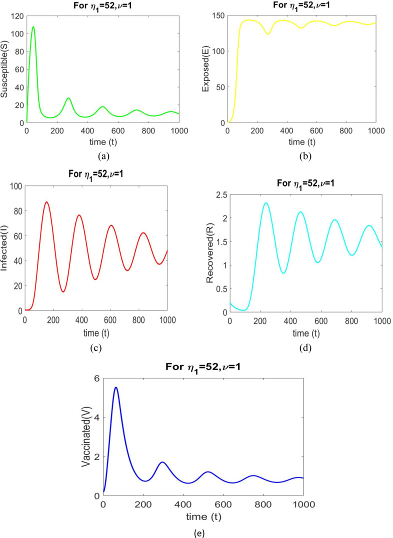
The values of the parameters in Table 3 are used to study the bifurcation analysis. The model system (2.9) is unstable at $E_1$, as shown in Fig. 11.

Parameters	Value	Source
$\Lambda$	5	For model fit
$\beta$	0.010	Estimated
${\mu }_0$	0.025	Estimated
$\delta$	0.002	Model to fit
${\mu }_1$	0.009	Estimated
${\mu }_2$	0.0008	For model fit

Fig. 11.

Time series solution of the model system (2.9) for ${\eta }_1>{{\eta }_1}^{\ast },\nu =1$ with different initial and parameter values as given in Table 3.

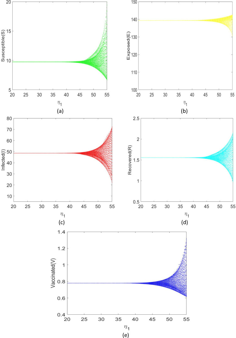
Using the parametric values in Table 3, the roots of the Eq. (3.10) are $-0.6240,-1.2724,0.1345,0.5832\pm 0.1750i$. Thus we obtain $f_1^{\prime }\left(0.1345\right)\ne 0$. The Hopf bifurcation diagram is shown in Fig. 12(a) through 12 (e). For ${\eta }_1=41.56$ and $m_{10}=0.3668$, we obtain $E_1=(9.7467,379.4148,132.3540,10.5883,0.7797)$. Now $E_1$ is locally asymptotically stable when ${\eta }_1\in [0,{{\eta }_1}^{\ast }]$, confirming our theoretical results in Theorem 3.5. The system (2.9) produces a Hopf bifurcation when ${\eta }_1={{\eta }_1}^{\ast }$.

Fig. 12.

Diagram of a single parameter bifurcation with respect to ${\eta }_1$.

6. Conclusion

We have studied the $\mathit{SEIRV}$ model (2.9) considering a single time delay parameter ${\eta }_1$. The stability analysis of the system depicts that point $E_0$ of the system (2.9) is locally asymptotically stable when ${\mathfrak{R}}_0$< 1, and unstable when ${\mathfrak{R}}_0>1$ in the absence of time delay. The endemic equilibrium $E_1=(S^{\ast },E^{\ast },I^{\ast },R^{\ast },V^{\ast })$ is locally asymptotically stable if ${\mathfrak{R}}_0>1$, when ${\eta }_1=0$. However, in the presence of time delay parameter ${\eta }_1$, both the points $E_0$ and $E_1$ are asymptotically stable in the interval $[0,{{\eta }_1}^{\ast }]$ where ${{\eta }_1}^{\ast }$ is given by ${{\eta }_1}^{\ast }=\frac{1}{m_{10,}}si{n}^{-1}\left(\frac{ad+bc}{a^2+b^2}\right)$. Numerical computations reveal that if ${\eta }_1>41.56$ then the system (2.9) exhibits Hopf bifurcation. Thus, it becomes apparent that beyond the value of ${{\eta }_1}^{\ast }=41.56$ the dynamics of the system becomes unstable. It may be recalled that the time delay parameter was incorporated in (2.9) to justify the argument that the infected population will take some time to recover. When the time delay owing to the time period required by the infected individuals to recover from the disease surpasses a threshold value, the model described here produces a Hopf bifurcation around the endemic equilibrium point.

Declaration of Competing Interest

The authors declare that they have no known competing financial interests or personal relationships that could have appeared to influence the work reported in this paper.

References

- 1.Gumel A.B., Mccluskey C., Watmough J. An SVEIR model for assessing potential impact of an imperfect anti-SARS vaccine. Math Biosci Eng. 2006;3(3):485–512. doi: 10.3934/mbe.2006.3.485. [DOI] [PubMed] [Google Scholar]
- 2.Wang L., Xu R. Global stability of an SEIR epidemic model with vaccination. Int J Biomath. 2016;9(6):18–35. [Google Scholar]
- 3.Ji C., Jiang D., Shi N. Multigroup SIR epidemic model with stochastic perturbation. Physica A. 2011;390(10):1747–1762. [Google Scholar]
- 4.Liu M., Bai C., Wang K. Asymptotic stability of a two-group stochastic SEIR model with infinite delays. Commun Nonlinear Sci Numer Simul. 2014;19(10):3444–3453. [Google Scholar]
- 5.Roy R., Akbar M.A., Seadawy A.R., Baleanu D. Search for adequate closed form wave solutions to space–time fractional nonlinear equations. Partial Differ Equ Appl Math. 2021;3 doi: 10.1016/j.padiff.2021.100025. [DOI] [Google Scholar]
- 6.Yang Q., Mao X. Extinction and recurrence of multi-group SEIR epidemic models with stochastic perturbations. Nonlinear Analysis RWA. 2013;14(3):1434–1456. [Google Scholar]
- 7.Yu J., Jiang D., Shi N. Global stability of two-group SIR model with random perturbation. J Math Anal Appl. 2009;360(1):235–244. [Google Scholar]
- 8.Din A., Khan F.A., Khan Z.A., Yusuf A., Munir T. The mathematical study of climate change model under nonlocal fractional derivative. Partial Differ Equ Appl Math. 2021;5 doi: 10.1016/j.padiff.2021.100204. [DOI] [Google Scholar]
- 9.Tang B., Wang X., Li Q., et al. Estimation of the transmission risk of the 2019-nCoV and its implication for public health interventions. J Clin Med. 2020;9(2):462. doi: 10.3390/jcm9020462. [DOI] [PMC free article] [PubMed] [Google Scholar]
- 10.Frank T.D., Chiangga S. SEIR order parameters and eigenvectors of the three stages of completed COVID-19 epidemics: with an illustration for Thailand January to 2020. Phys Biol. 2021;18(4) doi: 10.1088/1478-3975/abf426. [DOI] [PubMed] [Google Scholar]
- 11.Rothe C., Schunk M., Sothmann P., et al. Transmission of 2019-nCoV infection from an asymptomatic contact in Germany. N Engl J Med. 2020;382(10):970–971. doi: 10.1056/NEJMc2001468. [DOI] [PMC free article] [PubMed] [Google Scholar]
- 12.Lu H., Stratton C.W., Tang Y.W. Outbreak of pneumonia of unknown etiology in Wuhan, China: the mystery and the miracle. J Med Virol. 2020;92(4):401–402. doi: 10.1002/jmv.25678. [DOI] [PMC free article] [PubMed] [Google Scholar]
- 13.Vattay G. Forecasting the outcome and estimating the epidemic model parameters from the fatality time series in COVID-19 outbreaks. Phys Biol. 2020;17(6) doi: 10.1088/1478-3975/abac69. [DOI] [PubMed] [Google Scholar]
- 14.Derakhshan M.H. The stability analysis and numerical simulation based on sinc Legendre collocation method for solving a fractional epidemiological model of the Ebola virus. Partial Differ Equ Appl Math. 2021;3 doi: 10.1016/j.padiff.2021.100037. [DOI] [Google Scholar]
- 15.Billy Quilty J., Clifford S., et al. Effectiveness of airport screening at detecting travellers infected with novel coronavirus (2019-ncov) Euro Surveillance. 2020;25(5) doi: 10.2807/1560-7917.ES.2020.25.5.2000080. [DOI] [PMC free article] [PubMed] [Google Scholar]
- 16.Wang H., Wang Z., Dong Y., Chang R., et al. Phase-adjusted estimation of the number of coronavirus disease 2019 cases in Wuhan, China. Cell Discov. 2020;6(10):PMC7039910. doi: 10.1038/s41421–020–0148–0. [DOI] [PMC free article] [PubMed] [Google Scholar]
- 17.Ferretti L, Wymant C, Kendall M et al. Quantifying SARS-CoV-2 transmission suggests epidemic control with digital contact tracing, 2020;368(6491):eabb6936. 10.1126/science.abb6936. [DOI] [PMC free article] [PubMed]
- 18.Paul S., Mahata A., Mukherjee S., Roy B. Dynamics of SIQR epidemic model with fractional order derivative. Partial Differ Equ Appl Math. 2022;5 doi: 10.1016/j.padiff.2021.100216. [DOI] [PMC free article] [PubMed] [Google Scholar]
- 19.Zhao S., Lin Q., Ran J., et al. Preliminary estimation of the basic reproduction number of novel coronavirus in China, from 2019 to 2020: A data-driven analysis in the early phase of the outbreak. Int J Infect Dis. 2020;92:214–217. doi: 10.1016/j.ijid.2020.01.050. [DOI] [PMC free article] [PubMed] [Google Scholar]
- 20.Wu Joseph T., Leung Kathy, Leung Gabriel M. Now casting and forecasting the potential domestic and international spread of the 2019-ncov outbreak originating in Wuhan, China: a modelling study. Lancet. 2020;395(10225):689–697. doi: 10.1016/S0140-6736(20)30260-9. [DOI] [PMC free article] [PubMed] [Google Scholar]
- 21.Paul S., Mahata A., Ghosh U., Roy B. SEIR epidemic model and scenario analysis of COVID-19 pandemic. Ecol Genet Genom. 2021;19 doi: 10.1016/j.egg.2021.100087. [DOI] [PMC free article] [PubMed] [Google Scholar]
- 22.Kuang Y. Academic Press Inc; 1993. Delay Differential Equations with Applications in Population Dynamics. [Google Scholar]
- 23.Brauer F., Castillo-Chavez C. Springer; 2001. Mathematical Models in Population Biology and Epidemiology. Vol. 40. [Google Scholar]
- 24.Xu C., Liao M., Li P., Guo Y., Xiao Q., Yuan S. Influence of multiple time delays on bifurcation of fractional-order neural networks. Appl Math Comput. 2019;361:565–582. [Google Scholar]
- 25.Xu C., Liu Z., Liao M., Li P., Xiao Q., Yuan S. Fractional-order bidirectional associate memory (BAM) neural networks with multiple delays: The case of Hopf bifurcation. Math Comput Simul. 2021;182:471–494. doi: 10.1016/j.matcom.2020.11.023. [DOI] [Google Scholar]
- 26.Xu C., Liu Z., Yao L., Aouiti C. Further exploration on bifurcation of fractional-order six-neuron bi-directional associative memory neural networks with multi-delays. Appl Math Comput. 2021;410 doi: 10.1016/j.amc.2021.126458. [DOI] [Google Scholar]
- 27.Xu C., Liao M., Li P., et al. Bifurcation properties for fractional order delayed BAM neural networks. Cogn Comput. 2021;13:322–356. doi: 10.1007/s12559-020-09782-w. [DOI] [Google Scholar]
- 28.Xu C., Zhang W., Aouiti C., Liu Z., Liao M., Li P. Further investigation on bifurcation and their control of fractional-order bidirectional associative memory neural networks involving four neurons and multiple delays. Math Methods Appl Sci. 2021;1–24 [Google Scholar]
- 29.Xu C., Liao M., Li P., Yuan S. Impact of leakage delay on bifurcation in fractional-order complex-valued neural networks. Chaos Solitons Fractals. 2021;142 [Google Scholar]
- 30.Xu C., Zhang W., Liu Z., Yao L. Delay-induced periodic oscillation for fractional-order neural networks with mixed delays. Neurocomputing. 2021 doi: 10.1016/j.neucom.2021.11.079. [DOI] [Google Scholar]
- 31.J. Liu. Bifurcation of a delayed SEIS epidemic model with a changing delitescence and nonlinear incidence rate. Discrete Dyn Nat Soc. 2017;1–9 [Google Scholar]
- 32.Liu J., Wang K. Hopf bifurcation of a delayed SIQR epidemic model with constant input and nonlinear incidence rate. Adv Differential Equations. 2016;168:20. [Google Scholar]
- 33.Sun X., Wei J. Stability and bifurcation analysis in a viral infection model with delays. Adv Differential Equations. 2015;332:22. [Google Scholar]
- 34.Krishnariya P., Pitchaimani M., Witten T.M. Mathematical analysis of an influenza a epidemic model with discrete delay. J Comput Appl Math. 2017;324:155–172. [Google Scholar]
- 35.Liu Q., Chen Q.M., Jiang D.Q. The threshold of a stochastic delayed SIR epidemic model with temporary immunity. Physica A. 2016;450:115–125. [Google Scholar]
- 36.Bai Z.G., Wu S.L. Traveling waves in a delayed SIR epidemic model with nonlinear incidence. Appl Math Comput. 2015;263:221–232. [Google Scholar]
- 37.Liu Q.M., Deng C.S., Sun M.C. The analysis of an epidemic model with time delay on scale-free networks. Physica A. 2014;410:79–87. [Google Scholar]
- 38.Xu R., Zhang S., Zhang F. Global dynamics of a delayed SEIS infectious disease model with logistic growth and saturation incidence. Math Methods Appl Sci. 2016;39:3294–3308. [Google Scholar]
- 39.Jiang Z.C., Ma W.B., Wei J.J. Global Hopf bifurcation and permanence of a delayed SEIRS epidemic model. Math Comput Simulation. 2016;122:35–54. [Google Scholar]
- 40.Chen X.Y., Cao J.D., Park J.H., et al. Stability analysis and estimation of domain of attraction for the endemic equilibrium of an SEIQ epidemic model. Nonlinear Dynam. 2017;87:975–985. [Google Scholar]
- 41.Kilbas A., Srivastava H., Trujillo J. Theory and applications of fractional differential equations. North-Holland Math Stud. 2006;204:1–523. [Google Scholar]
- 42.Caputo M., Fabrizio M. A new definition of fractional derivative without singular kernel. Prog Fract Differ Appl. 2015;1(2):73–85. [Google Scholar]
- 43.Liang S., Wu R., Chen L. Laplace transform of fractional order differential equations. Electron J Differential Equations. 2015;2015(139):1–15. [Google Scholar]
- 44.Kexue L., Jigen P. Laplace transform and fractional differential equations. Appl Math Lett. 2011;24(12):2019–2023. [Google Scholar]
- 45.Petras I. Higher Education Press; Beijing, China: 2011. Fractional-Order Nonlinear Systems: Modeling Aanlysis and Simulation. [DOI] [Google Scholar]
- 46.Upadhyay R.K., Kumari S., Misra A.K. Modeling the virus dynamics in computer network with SVEIR model and nonlinear incident rate. J Appl Math Comput. 2017;54:485–509. doi: 10.1007/s12190-016-1020-0. [DOI] [Google Scholar]
- 47.Zhang Z., Kundu S., Tripathi J.P., Bugalia S. Stability and Hopf bifurcation analysis of an SVEIR epidemic model with vaccination and multiple time delay. Chaos Solitons Fractals. 2019;131 doi: 10.1016/j.chaos.2019.109483. [DOI] [Google Scholar]
- 48.Pongkitivanichkul C., Samart D., Tangphati T., et al. Estimating the size of COVID-19 epidemic outbreak. Phys Scr. 2020;95(8) [Google Scholar]
- 49.Zhu L.H., Wang X.W., Zhang H.H., Shen S.L., Li Y.M., Zhou Y.D. Dynamics analysis and optimal control strategy for a SIRS epidemic model with two discrete time delays. Phys Scr. 2020;95(3) [Google Scholar]
- 50.Perko L. Springer; 2000. Differential Equations and Dynamical Systems. [DOI] [Google Scholar]
- 51.Li M.Y., Smith H.L., Wang L. Global dynamics of an SEIR epidemic model with vertical transmission. SIAM J Appl Math. 2001;62(1):58–69. [Google Scholar]
- 52.Hassard B.D., Kazarinoff N.D., Wan Y.H. Cambridge University Press; Cambridge: 1981. Theory and Applications of Hopf Bifurcation; pp. 300–309. [Google Scholar]
- 53.India COVID-19 Tracker. https://www.covid19india.org/2020.
- 54.https://www.worldometers.info/coronavirus/.