SCAN‐Clim: a tool to support pest climate suitability analysis based on climate classification

Abstract

EFSA pest categorisations and pest risk assessments include the assessment of the potential establishment of plant pests. Together with the presence of host plants, climate suitability analysis is an important element to analyse the likelihood of potential establishment of a pest in an area. One of the main approaches used in EFSA plant health risk assessment is the analysis based on climate classifications i.e. evidencing the occurrence of climates enhancing pest development and persistence in a specific area. SCAN‐Clim is a tool designed to support climate suitability analysis based on climate classifications. The current version is the first prototype of the tool, developed in the R language, currently used to support EFSA climate suitability analysis for pest categorisation and for quantitative pest risk assessment. Tested on over 34 EFSA works, SCAN‐Clim significantly improved the speed of climate suitability maps generation guaranteeing a standardised map format and providing documentation on input/outputs. Further improvements will include the development of an interactive web app accessible through the EFSA R4EU Portal (expected to be delivered in 2022).

1. Introduction

Climate suitability analysis is an important element to analyse the likelihood of potential establishment of a pest in an area (EFSA PLH Panel, 2018). Different approaches exist (e.g. Species Distribution Models, and CLIMEX) (Magarey et al., 2005; MacLeod and Korycinska, 2019; Early et al., 2021). One of them is based on the comparison between the climate in the known distribution of a pest and the ones in the area under pest risk assessment using climate classification maps like, e.g. the Köppen–Geiger classification. This methodology is widely used in the context of EFSA pest categorisations (in 2021, it was used in more than 30 Pest Categorisations) where simplified and succinct analyses are needed (e.g. EFSA PLH Panel, 2021a, 2021b, 2021c, 2021d). In fact, in the context of EFSA pest categorisations, due to time constraints, this approach has been commonly applied at the country level (i.e. using pest observations at the country level and considering all climates in the same country) and then refined if necessary. However, it can also be used for more detailed assessments using pest observations at higher resolution (e.g. province, grid reference coordinates or latitude/longitude). SCAN‐Clim is a tool designed to support climate suitability analysis based on climate classifications, i.e. evidencing the occurrence of climates in a specific area. This document describes the first prototype of the tool, developed using the R language (R Core Team, 2017) in the RStudio platform (RStudio Team, 2020).

1.1. Background and Terms of Reference as provided by the requestor

EFSA is requested, pursuant to Article 29(1) of Regulation (EC) No 178/2002, to provide scientific opinions in the field of plant health.

EFSA is requested to deliver 53 pest categorisations for the pests listed in Annexes 1A, 1B, 1D and 1E (for more details see mandate M‐2021‐00027 on the Open.EFSA portal). Additionally, EFSA is requested to perform pest categorisations for the pests so far not regulated in the EU, identified as pests potentially associated with a commodity in the commodity risk assessments of the High Risk Plants (HRP) dossiers (Annex 1C; for more details see mandate M‐2021‐00027 on the Open.EFSA portal). Such pest categorisations are needed in the case where there are not available risk assessments for the EU.

When the pests of Annex 1A are qualifying as potential Union quarantine pests, EFSA should proceed to phase 2 risk assessment. The opinions should address entry pathways, spread, establishment, impact and include a risk reduction options analysis.

Additionally, EFSA is requested to develop further the quantitative methodology currently followed for risk assessment, in order to have the possibility to deliver an express risk assessment methodology. Such methodological development should take into account the EFSA Plant Health Panel Guidance on quantitative pest risk assessment and the experience obtained during its implementation for the Union candidate priority pests and for the likelihood of pest freedom at entry for the commodity risk assessment of High Risk Plants.

1.2. Interpretation of the Terms of Reference

This Scientific Report describes a tool developed to support climate suitability analysis for the assessment of the probability of establishment in pest categorisation and pest risk assessment, following the indication of the EFSA Guidance on quantitative pest risk assessment (EFSA PLH Panel, 2018). The main objective of SCAN‐Clim is to ensure fast and reproducible climate suitability analysis based on climate classification in the context of pest risk assessment. SCAN‐Clim was developed to improve efficiency and the transparency of the climate suitability assessment process.

2. Data and methodologies

2.1. General description

SCAN‐Clim is a tool to support the development of climate suitability analysis based on climate classifications. The current version described in this document is a prototype and it was developed using the R language (R ≥ 4.0.5) (Table 1). It was designed for users with none or very basic knowledge of R or programming and with no knowledge on GIS. It requires the installation of the software R and RStudio and of specific R packages. The current state of development requires some initial support for the installation and update of specific R packages for users not familiar with R. However, after the installation process is completed, no more support is needed to run the tool.

Table 1.

SCAN‐Clim technical specifications

Title	SCAN‐Clim – Supporting Climate suitAbility aNalysis based on Climate Classifications
Version	1.0
Date	November 2021
R version	≥ 4.0.5
Needed R packages (installed automatically by the tool if not yet installed)	sp (≥ 1.4.5), raster (≥ 3.4.10), readxl (≥ 1.3.1), httr (≥ 1.4.2), XML (≥ 3.99), rlist (≥ 0.4.6.1), rmarkdown (≥ 2.8), knitr (≥ 1.33), rasterVis (0.50.2), latticeExtra (0.20–44), rgeos (0.5–5)
Description	Tool to support pest climate suitability analysis based on climate classification
Authors	Andrea Maiorano
Review and testing	Caterina Campese
Maintainer	Andrea Maiorano andrea.maiorano@efsa.europa.eu
License agreement	Creative Commons Attribution 4.0
Link to software	https://doi.org/10.5281/zenodo.5780031

The tool is published in Zenodo in the EFSA Knowledge Junction community, this report refers to version 1 (https://doi.org/10.5281/zenodo.5780031). Two versions are available, one for Windows users and the other for Mac users.

2.2. Elements and data included in SCAN‐Clim

In this section, a list and description of the elements/data included in the tool are shown. Next section shows how they are connected in the tool and the interaction with the user.

2.2.1. Raster file with the climate classification map

Currently, SCAN‐Clim output is based on the Köppen–Geiger classification based on the period 1986–2010 (25‐year period) and on a 10‐km grid from the Institute for Veterinary Public Health of the University of Vienna based on Kottek et al. (2006) rescaled after Rubel et al. (2017)1 (Figure 1). However, SCAN‐Clim can be easily updated with different climate classifications (similar raster files).

Figure 1.

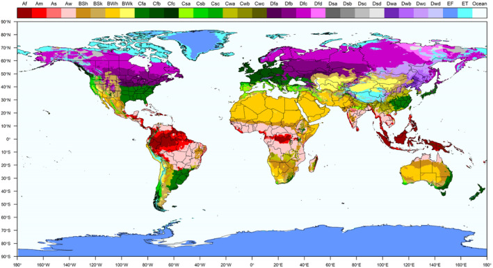
Köppen–Geiger climate classification. Different colours represent different climates. Climates are described in the top legend with a standard two or three letter code

2.2.2. GIS layers including administrative boundaries of the world at different administrative unit level (country to province/county)

Administrative boundary layers are used to identify areas of observation of the organism.

Available layers include the Global Administrative Unit Layers (GAUL) dataset, implemented by the Food and Agriculture Organisation of the United Nations (FAO) within the CountrySTAT and Agricultural Market Information System (AMIS) projects, and a layer (based on the FAO GAUL layers) including the administrative units used by the European and Mediterranean Plant Protection Organization (EPPO).

Layers from FAO (GAUL):

• FAO GAUL level 0: Country level

• FAO GAUL level 1: Region level (or states for big countries like US, China, Brazil or Canada)

• FAO GAUL level 2: province/county level

Layer based on the EPPO administrative subdivision:

• EPPO‐like layer: This is a layer based on the FAO GAUL level 0 but including further subdivisions for certain countries compared to FAO GAUL level 0 (e.g. for Russian Federation, US, China, India, etc…)

All the layers are included as RData files (i.e. a data format designed for R) in the Data/rdata folder. Figure 2 shows three examples of available layers.

Figure 2.

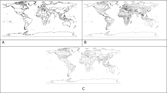
Examples of layers for administrative units at different administrative level. A = FAO GAUL level 0; B = FAO.GAUL level 1; C = EPPO‐like administrative layer

2.2.3. List of relevant climates for the organism

The list of the climates that are relevant for the organism can be either defined by the user or automatically extrapolated by SCAN‐Clim based on distribution (Section 2.4).

2.2.4. List of organism geographic distribution

The list of pest geographic distribution can be defined by the user or downloaded from the EPPO global database (Section 2.4). The pest distribution in the EPPO global database is at the country level. The user can define the geographic distribution at different levels, from the country to the province/county, or even single point if geographic coordinates are provided.

2.3. Structure and description of the source package

The tool is distributed as a source package organised in folders including files and subfolders. Figure 3 shows the structure of the source package whose use is described in detail in Section 2.4. Table 2 describes the content of the main folder, including files and subfolders and specifying which of them are intended to support the functionalities of the tool or which are to be used, opened or modified by the user. An R expert user can modify any of the files included in the tool.

Figure 3.

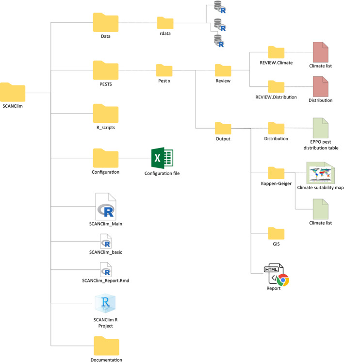
Structure of the SCAN‐Clim source package

Table 2.

Content of the main SCAN‐Clim folder. In grey files and folders which include interaction with the user

File/Folder	Name	Description	User interaction
Folder	Data	Includes R data files with spatial data (climate classification raster, administrative units layers)	No
Folder	R_scripts	Includes R scripts	No
Folder	Documentation	Includes csv files with tables with information useful to run the tool	Yes
Folder	Configuration	Includes the SCAN‐Clim Excel configuration file	Yes
Folder	PESTS	For each analysed pest includes a folder with outputs of SCAN‐Clim	Yes
File	SCAN‐Clim. Rproj	R Project file. The RStudio session must be opened with this file (more information below)	Yes
File	SCAN‐Clim_Main.r	From the RStudio session, this is the only file that must be opened. User only need to run the script by clicking on the button ‘source’. (more information below	Yes
File	SCAN‐Clim_basic.r	R file that run the basic version of the tool (i.e. no automatic reporting)	No
File	SCAN‐Clim_Report. Rmd	R file that run the version of the tool that outputs also an html report	No

2.3.1. Data/rdata folder

The data folder includes RData files including mapping elements of SCAN‐Clim.

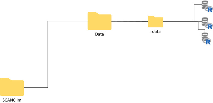
Figure 4. SCAN‐Clim Data folder (detail from Figure  3 )

No user interaction is required for running the tool.

2.3.2. PESTS folder

Every time that SCAN‐Clim is run for an organism, a folder called with the name of the organism is automatically created inside the folder PESTS. This folder includes the folders Output and Review.

2.3.3. PESTS folder: Output subfolder

The Output folder is the folder where users can find the outputs of SCAN‐Clim. It includes:

• – an html report including the main outputs (distribution, relevant climates and the Köppen–Geiger map of the organism in a low resolution, for illustration purposes).
• – the Output/Koppen–Geiger folder with the climate suitability map at high resolution and the list of relevant climates
• – the Output/Distribution folder includes the EPPO distribution table for the organism in csv format. The EPPO distribution table is saved only if no user‐defined distribution table was saved in the REVIEW.Distribution folder (see Section 2.4)
• – the Output/GIS folder, including raster and shapefiles of the maps that can be used in GIS software

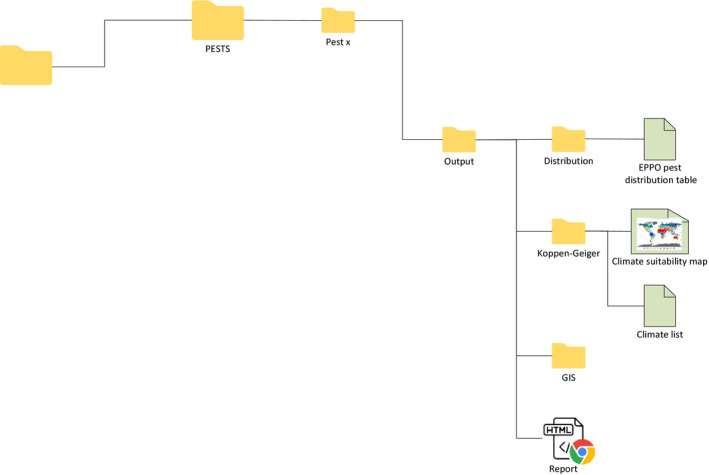
Figure 5. SCAN‐Clim Output subfolder of the PESTS/[Pest.name] folder (detail from Figure  3 )

2.3.4. PESTS folder: Review subfolder

In the Review subfolder (Figure 6), users can save csv files specifying the list of climates that are to be included in the map, or a user‐defined distribution table:

• – in the folder REVIEW.Climates users can save the list of climates that are to be included in the assessment. If such a list is included, SCAN‐Clim will use only this list for the final output. The file must be a csv file with one column and one header called ‘Climate’
• – the folder REVIEW.Distribution where users can save a user‐defined distribution table. The table can include entries at different administrative unit level (Country, Region, and/or county/province) or at the point level specifying geographic coordinates. A facsimile distribution table is available in the Documentation folder.

Figure 6.

SCAN‐Clim Output Review subfolders of the PESTS/[Pest.name] folder (detail from Figure  3 )

2.3.5. Configuration folder

The Configuration folder includes the SCAN‐Clim Excel configuration file with different type of input in each sheet:

• Authors sheet: List of authors to be included in the final html report.

• Pest_list sheet: List of organisms (scientific name) to be analysed.

• Pest_status_to_be_included sheet: Type of observations from the EPPO observed distribution table to be considered in the analysis. Default list includes: ‘Present, no details’, ‘Present, widespread’, ‘Present, restricted distribution’, ‘Present, few occurrences’. This is relevant only if SCAN‐Clim connect to the EPPO Global database, i.e. a distribution table is not provided by the user.

• Climates_to_be_removed sheet: List of climates generally not relevant for the analysis. Default includes ‘Ocean’.

• Other settings sheet: user can select.

  • ○ Remove from the output all the climates not present in EU (yes/no).
  • ○ Select region to map: dropdown list currently includes Global, America, Asia, Australia, Caribbean, Europe, Oceania, USA, Peru, South East Asia, China, South East China. Other countries or specific regions can be added (contact the developer).
  • ○ Recalculate EU27 climate list: yes/no. In the case a new climate classification map is used, the recalculation is necessary.
  • ○ EPPO API token: To connect to the EPPO Global database users need to have an account registered in the EPPO Data Services (https://data.eppo.int/). After login, the token can be copied from the personal home page.
  • ○ Print html report (yes/no). Selecting ‘no’ reduces the time for map generation to around 40–45 s
  • ○ Save GIS layers (yes/no).

• Tech sheet (hidden sheet): hidden sheet, not to be modified by the user, including info/data needed for the dropdown menus included in the configuration file itself.

2.4. Running SCAN‐Clim: scenarios of analysis

Figure 7 shows a general representation of the tool workflow. There are basically four main scenarios to run the tool based on the information given as input: (1) Basic configuration, (2) climate list defined by the user, (3) pest distribution defined by the user, (4) climate list and pest distribution defined by the user. The steps included in the basic configuration are common to all the scenarios.

Figure 7.

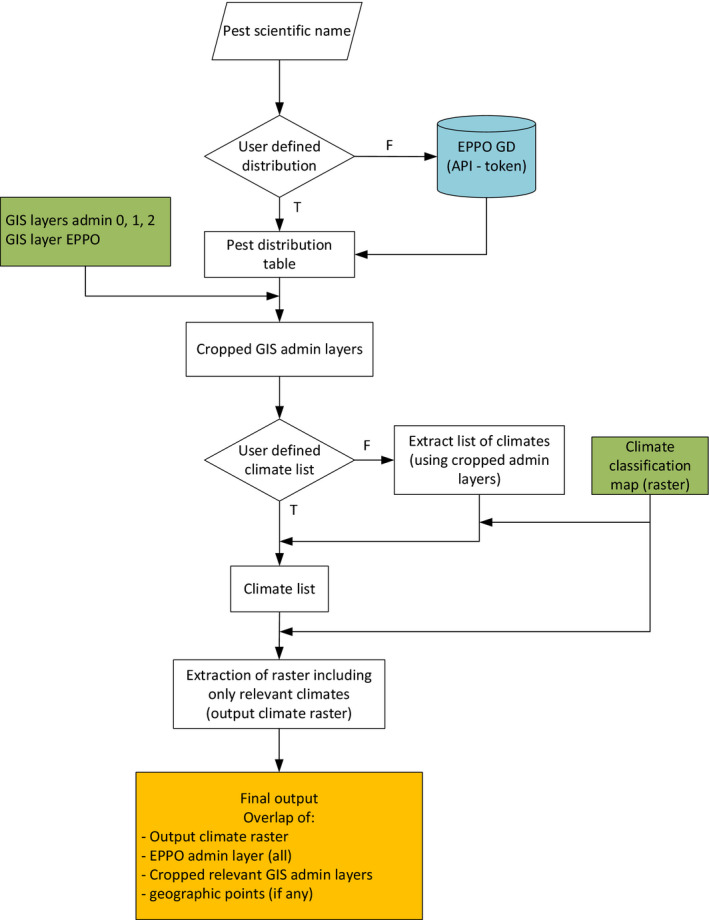
SCAN‐Clim general workflow

2.4.1. Basic configuration

In the Basic configuration, the only needed input is the scientific name of the organism under assessment. SCAN‐Clim connects to the EPPO Global Database through a dedicated REST API (https://data.eppo.int/documentation/rest, registration and token is needed), downloads the pest distribution table, retrieves the list of relevant climates overlapping the cropped administrative layers (based on the distribution list) and the Köppen–Geiger raster file and outputs a climate suitability map based on information at country level (i.e. resolution of EPPO GD distribution table). In Table 3, a step‐by‐step guide to run SCAN‐Clim is available.

Table 3.

Steps for running the basic configuration of SCAN‐Clim

Step #	Step description	File
01	Open the configuration file Open Pest_list sheet and write the scientific name(s) of the organism(s) Optionally fill the Authors excel sheet	Configuration folder, Excel file
02	Double click on the SCAN‐Clim. Rproj file (R project file). The tool should always be opened from this file as this open an R Studio session based on the file system of the tool. If file extensions are not visible, the name of the file is just SCAN‐Clim and it is the file with the icon shown in this table
03	A R Studio session opens. – Focus on the bottom‐right panel (black rectangle). – Check that the main SCAN‐Clim directory is selected or navigate to it (step 1, red rectangle) – Single click on the SCAN‐Clim_Main.r file (step 2, blue rectangle) – Click on the button Source to run the tool (step 3, orange rectangle)

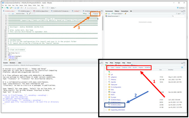
2.4.2. User‐defined climate types list

Before the steps described for the Basic configuration, users can specify the list of climates to be included in the final output in a.csv file, including a single column with header ‘climates’ and the list of the codes of the climates. Figure 8 shows an example file opened in Windows Notepad. An example.csv file is also included in the folder Documentation. Such file is to be saved in the folder PESTS/[Pest name]/Review/REVIEW. Climate. The steps described in the Basic configuration are then to be executed.

Figure 8.

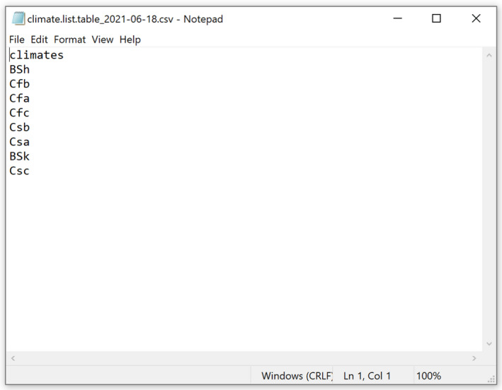
Example.csv file including the list of climates to be mapped. The file is shown as visualised in Windows Notepad

SCAN‐Clim connects anyway to the EPPO Global Database to retrieve the distribution table, but the climates shown in the final map are the ones listed by the user.

2.4.3. User‐defined pest distribution

Before the steps described for the Basic configuration user can define a pest distribution table in a.csv file which is to be saved in the folder PESTS/[pest.name]/Review/REVIEW. Distribution.

An example distribution file is included in the Documentation folder, however, if the tool is firstly run with the basic configuration, a distribution table is automatically created including the records from the EPPO Global Database and is saved in the folder PESTS/[pest.name]/Output/Distribution. This table can be copied and pasted to the review folder and modified with user defined occurrences.

The table must include the fields listed below. Not all the fields need to be filled in for the correct running of the tool; however, they are present for completeness of information on the pest occurrence records:

• – Continent: Filling not essential
• – Country: Filling not essential
• – State: Filling not essential
• – Observation: Filling not essential, this field include the name of the administrative unit where the organism was observed
• – admin.source: This field can include three values: ‘EPPO’, ‘FAO.GAUL’ or ‘location’. See below for more information
• – admin.code: This field should include the FAO.GAUL administrative unit codes. Codes are available in the FAO_GAUL_Codes_and_names.csv available in the Documentation folder.
• – lat: Latitude in decimal degrees (in the case of ‘location’ occurrences)
• – long: Longitude in decimal degrees (in the case of ‘location’ occurrences)

Here is a step‐by‐step instruction on how to fill the distribution table:

1. if SCAN‐Clim was run with the basic configuration a distribution table in the Output folder can be used. This table will already include EPPO records (country level). User can decide to keep those records or remove them.

2. In the case specific location occurrences are available, indicate ‘location’ in the admin.source field, and geographic coordinates in the lat and long fields

3. In the case occurrences refer to administrative units (from the country level to the province/county level), indicate ‘FAO.GAUL’ in the admin.source field, the name of the administrative unit in the Observation field and the FAO GAUL administrative code in the admin.code field. If the administrative code is not indicated SCAN‐Clim run anyway trying to match the names indicated in the Observation fields with the names included in the geographic layers used for mapping. However, it is strongly recommended to specify the administrative code as it is highly possible that for some reason (e.g. local name vs. international name, accents, machine international configurations), the names do not match. The administrative codes can be found in the FAO_GAUL_Codes_and_names.csv file available in the Documentation folder. This file includes a table with the different names and codes of the GAUL administrative units, organised per administrative unit level: 0 = Country, 1 = Region, 2 = Province/County.

If a user‐defined climate list was not included (see previous paragraph), the Köppen–Geiger climates are extracted using the user‐defined distribution.

2.5. SCAN‐Clim outputs html report

SCAN‐Clim outputs an html report saved in the folder PESTS/[pest name]/Output which includes the observation table, a table including the list of climates (and their description) extracted based on the observations and a map in low resolution just for checking purposes. In the case of observation records not recognised by the tool (and consequently not used to extract the climates), a specific paragraph called Observed distribution is automatically added to the report including the list of location names that need to be checked. In this case, it is recommended to rerun the tool with a user‐defined distribution table using the FAO.GAUL codes and names for the not recognised records (see previous paragraph).

3. Results and Discussion

A run of the tool with a global map selected as preferred output and also including the print of the html report requires on average around 1 min. This time can vary mainly in relation to the PC configuration (processor and RAM available, ±15 s), and to the output options selected by the user. For instance, no printing the html report can save around 15 s. Outputting a map only for a selected region (e.g. Europe) instead of a global map can save additional 20 s. Hence, time for running the tool can be shortened to 30 s. Before the introduction of SCAN‐Clim, the development of such maps using GIS software required from 15 to 30 min depending on the number of pest observations (Czwienczek E., personal communication).

The tool was used for the first time for the EFSA Pest categorisation of the Colorado potato beetle Leptinotarsa decemlineata, a pest of potato (EFSA PLH Panel, 2020). In that case the experts required to highlight in the same map the EU protected zones for this pest (as per Regulation 2019/2072, (Annex III)). Adding new lawyers to the SCAN‐Clim output map can be done easily either in R (for R users) or using the GIS layers outputs of the tool.

So far, SCAN‐Clim has been used in the context of 15 published EFSA Scientific Opinions, 18 ongoing EFSA pest categorisations (Appendix A) and at the time of the writing of this document is being used also for the climate suitability analysis of two ongoing pest risk assessments. In all the published Scientific Opinions, SCAN‐Clim ensured to have climate suitability maps with a standard format as it is shown as examples in Figures 9 and 10 showing the output maps for two distinct pests.

Figure 9.

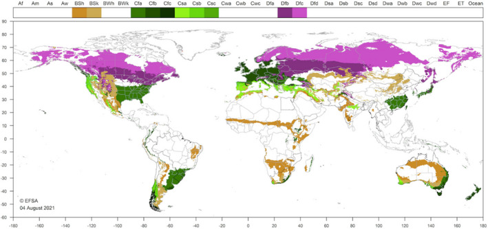
Climate suitability map from the EFSA Pest Categorisation of Oligonychus mangiferus (EFSA PLH Panel, 2021c)

Figure 10.

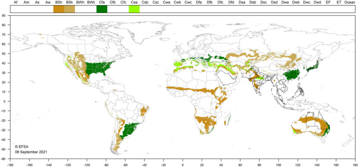
Climate suitability map from the EFSA Pest Categorisation of Leucinodes orbonalis (EFSA PLH Panel, 2021d)

4. Conclusions and future developments

SCAN‐Clim significantly improves the speed of map generation guarantying a standardised map format and providing documentation about input, output data and the review process by the users or working groups. In this way, the process is also transparent to experts, risk assessors and risk managers examining process of pest categorisation to further improve it.

SCAN‐Clim is under continuous development. The current version is being distributed to EFSA staff, to support working group activities, under developer assistance in order to fix minor bugs and to improve usability. External users can refer to the developer to have assistance.

Further improvement includes the development of an interactive web app based on R Shiny which will be accessible through the EFSA R4EU Portal (expected to be delivered in 2022). This version will greatly improve usability.

5. Recommendations

Cautionary note on the use of the tool

This tool allows the user to match climates in areas of known presence of a pest and climates in other parts of the world where the organism does not occur. The quality of the climate matching depends on the resolution of the source data, and it is user’s responsibility the correct use of the tool, and the interpretation of the results for instance by checking the consistency with observations and the organism biology and physiology.

Abbreviations

SCAN‐Clim

Supporting Climate suitability analysis based on Climate Classifications

EPPO

European and Mediterranean Plant Protection Organization

FAO

Food and Agriculture Organization of the United Nations

GAUL

Global Administrative Unit Layers

HRP

High Risk Plants

Appendix A – List of published and ongoing EFSA works supported by SCANClim

Table A.1 List of published Scientific Opinions supported by SCAN‐Clim

#	Scientific Opinion	Published
1	Pest categorisation of Oligonychus mangiferus	30 November 2021
2	Pest categorisation of Crisicoccus pini	26 November 2021
3	Pest categorisation of Leucinodes orbonalis	12 November 2021
4	Pest categorisation of Fusarium brachygibbosum	12 November 2021
5	Pest categorisation of Colletotrichum plurivorum	10 November 2021
6	Pest categorisation of Leucinodes pseudorbonalis	8 November 2021
7	Pest categorisation of Retithrips syriacus	8 November 2021
8	Pest categorisation of Colletotrichum fructicola	18 August 2021
9	Pest categorisation of Phenacoccus solenopsis	18 August 2021
10	Pest categorisation of Resseliella citrifrugis	12 August 2021
11	Pest categorisation of Phlyctinus callosus	3 August 2021
12	Pest categorisation of Elasmopalpus lignosellus	25 June 2021
13	Pest categorisation of Amyelois transitella	25 June 2021
14	Pest categorisation of Citripestis sagittiferella	25 June 2021
15	Commodity risk assessment of Ullucus tuberosus tubers from Peru	10 March 2021

Table A.2 List of ongoing EFSA pest categorisations with draft establishment section already supported by SCAN‐Clim

#	Scientific Opinion
1	Pseudococcus cryptus
2	Atalodera andina
3	Sirex nitobei
4	Plicosepalus acaciae
5	Malacosoma disstria
6	Fusarium oxysporum f. sp. cubense TR4
7	Penthimiola bella
8	Maconellicoccus hirsutus
9	Thecodiplosis japonensis
10	Arboridia kakogawana
11	Zaprionus indianus
12	Bagrada hilaris
13	Toumeyella parvicornis
14	Xanthomonas citri pv. viticola
15	Candidatus Liberibacter asiaticus
16	Matsucoccus massonianae
17	Matsucoccus matsumurae
18	Xylotrechus chinensis

Suggested citation: EFSA (European Food Safety Authority) and Maiorano A, 2022. Scientific Report on the SCAN‐Clim: a tool to support pest climate suitability analysis based on climate classification. EFSA Journal 2022;20(2):7104, 18 pp. 10.2903/j.efsa.2022.7104

References

- Early R, Rwomushana I, Chipabika G and Day R, 2021. Comparing, evaluating and combining statistical species distribution models and CLIMEX to forecast the distributions of emerging crop pests. Pest Management Science, 78, 671–683. [DOI] [PubMed] [Google Scholar]
- EFSA PLH Panel (EFSA Panel on Plant Health) , Michael J, Claude B, David C, Thierry C, Elisavet C, Katharina D‐S, Jean‐Claude G, Josep Anton JM, Alan M, Maria NN, Björn N, Stephen P, Roel P, Trond R, Vittorio R, Gregor U, Ariena VB, Wopke VDW, Jonathan W, Stephan W, Andy H, Jan S, Gritta S, Muriel S, Virag K, Svetla K, Maria Rosaria M, Olaf M‐S, Marco P, Giuseppe S, Sara T, Sybren V and Gianni G, 2018. Guidance on quantitative pest risk assessment. EFSA Journal, 2018;16(7):5356, 16 pp. 10.2903/j.efsa.2018.5356 [DOI] [Google Scholar]
- EFSA PLH Panel (EFSA Panel on Plant Health) , Bragard C, Dehnen‐Schmutz K, Di Serio F, Gonthier P, Jacques M‐A, Jaques Miret JA, Justesen AF, Magnusson CS, Milonas P, Navas‐Cortes JA, Parnell S, Potting R, Reignault PL, Thulke H‐H, Van der Werf W, Civera AV, Yuen J, Zappalà L, Kertesz V, Maiorano A, Streissl F and MacLeod A, 2020. Pest categorisation of Leptinotarsa decemlineata. EFSA Journal 2020;18(12):6359, 45 pp. 10.2903/j.efsa.2020.6359 [DOI] [PMC free article] [PubMed] [Google Scholar]
- EFSA PLH Panel (EFSA Panel on Plant Health) , Bragard C, Dehnen‐Schmutz K, Di Serio F, Gonthier P, Jacques M‐A, Jaques Miret JA, Justesen AF, MacLeod A, Magnusson CS, Milonas P, Navas‐Cortes JA, Parnell S, Potting R, Thulke H‐H, Van der Werf W, Civera AV, Yuen J, Zappalà L, Migheli Q, Vloutoglou I, Campese C, Maiorano A, Streissl F and Reignault PL, 2021a. Pest categorisation of Colletotrichum fructicola. EFSA Journal 2021;19(8):6803, 56 pp. 10.2903/j.efsa.2021.6803 [DOI] [PMC free article] [PubMed] [Google Scholar]
- EFSA PLH Panel (EFSA Panel on Plant Health) , Bragard C, Di Serio F, Gonthier P, Jaques Miret JA, Justesen AF, Magnusson CS, Milonas P, Navas‐Cortes JA, Parnell S, Potting R, Reignault PL, Thulke H‐H, Van der Werf W, Vicent Civera A, Yuen J, Zappalà L, Gregoire J‐C, Malumphy C, Campese C, Czwienczek E, Kertesz V, Maiorano A and MacLeod A, 2021b. Pest categorisation of Phlyctinus callosus. EFSA Journal 2021;19(8):6800, 45 pp. 10.2903/j.efsa.2021.6800 [DOI] [PMC free article] [PubMed] [Google Scholar]
- EFSA PLH Panel (EFSA Panel on Plant Health) , Bragard C, Di Serio F, Gonthier P, Jaques Miret JA, Justesen AF, Magnusson CS, Milonas P, Navas‐Cortes JA, Parnell S, Potting R, Reignault PL, Thulke H‐H, Van der Werf W, Vicent Civera A, Yuen J, Zappalà L, Gregoire J‐C, Malumphy C, Czwienczek E, Kertesz V, Maiorano A and MacLeod A, 2021c. Pest categorisation of Oligonychus mangiferus. EFSA Journal 2021;19(11):6927, 19 pp. 10.2903/j.efsa.2019.6927 [DOI] [PMC free article] [PubMed] [Google Scholar]
- EFSA PLH Panel (EFSA Panel on Plant Health) , Bragard C, Di Serio F, Gonthier P, Jaques Miret JA, Justesen AF, Magnusson CS, Milonas P, Navas‐Cortes JA, Parnell S, Potting R, Reignault PL, Thulke H‐H, Van der Werf W, Vicent Civera A, Yuen J, Zappalà L, Gregoire J‐C, Malumphy C, Czwienczek E, Maiorano A and MacLeod A, 2021d. Pest categorisation of Leucinodes orbonalis. EFSA Journal 2021;19(11):6890, 19 pp. 10.2903/j.efsa.2021.6890 [DOI] [PMC free article] [PubMed] [Google Scholar]
- Kottek M, Grieser J, Beck C, Rudolf B and Rubel F, 2006. World Map of the Köppen‐Geiger climate classification updated. Meteorologische Zeitschrif, 15, 259–263. [Google Scholar]
- MacLeod A and Korycinska A, 2019. Detailing Köppen‐Geiger climate zones at sub‐national to continental scale: a resource for pest risk analysis. EPPO Bulletin, 49, 73–82. [Google Scholar]
- Magarey RD, Sutton TB and Thayer CL, 2005. A simple generic infection model for foliar fungal plant pathogens. Phytopathology, 95, 92–100. [DOI] [PubMed] [Google Scholar]
- R Core Team , 2017. R: A language and environment for statistical computing. R Foundation for Statistical Computing, Vienna, Austria. Available online: https://www.R‐project.org/ [Google Scholar]
- RStudio Team , 2020. RStudio: Integrated Development Environment for R. RStudio, PBC, Boston, MA. Available online: https://www.rstudio.com/ [Google Scholar]
- Rubel F, Brugger K, Haslinger K and Auer I, 2017. The climate of the European Alps: shift of very high resolution Köppen‐Geiger climate zones 1800–2100. Meteorologische Zeitschrift, 26, 115–125. [Google Scholar]