Validation and demonstration of a new comprehensive model of Alzheimer’s disease progression

Abstract

Introduction:

Identifying the course of Alzheimer’s disease (AD) for individual patients is important for numerous clinical applications. Ideally, prognostic models should provide information about a range of clinical features across the entire disease process. Previously, we published a new comprehensive longitudinal model of AD progression with inputs/outputs covering 11 interconnected clinical measurement domains.

Methods:

Here, we (1) validate the model on an independent cohort; and (2) demonstrate the model’s utility in clinical applications by projecting changes in 6 of the 11 domains.

Results:

Survival and prevalence curves for two representative outcomes—mortality and dependency—generated by the model accurately reproduced the observed curves both overall and for patients subdivided according to risk levels using an independent Cox model.

Discussion:

The new model, validated here, effectively reproduces the observed course of AD from an initial visit assessment, allowing users to project coordinated developments for individual patients of multiple disease features.

1 |. INTRODUCTION

Despite our increased understanding of the neurobiological changes underlying Alzheimer’s disease (AD), it is still difficult to predict the rapidity of disease course for an individual patient, or accurately predict time to important milestones like need for nursing home care or death. This is most likely because of heterogeneity in the biological changes, genetics, and life exposures that are associated with the disease process. Accurately modeling the course of AD would generate information crucial for prognostic counseling of patients and their families, designing clinical trials in which the primary outcome is typically differential decline in cognitive and functional indices, and understanding the economic impact of the disease.

A complete model of disease progression should incorporate information about multiple clinical features acquired across the entire disease process. The model should be able to use data from an individual at a point in the disease process, and generate the likely future trajectory for that individual. To address this challenge, we previously introduced and demonstrated the internal validity of such a model based on a longitudinal grade of membership (L-GoM) approach to disease progression.¹ Using data from the Predictors 2 Study,² it incorporates measures of 11 key domains (see Table 1) at each patient’s initial visit and every 6 months for up to 10 years. Thus, it is a single comprehensive model of the entire disease process with the power to estimate the future prevalence of any of the incorporated disease features. Out-of-sample validation of this new model would provide the field with a highly flexible, widely applicable model to be used to optimize patient counseling, clinical trial design, genetic and biomarker studies, and economic models.

TABLE 1.

Domains of measurement, instruments, and descriptions of covariates used in the longitudinal grade of membership model

Domain	Instrument	Description of variables
Fixed covariates
	Initial assessment	ApoE status, sex, age at intake, race, occupation, years since diagnosis
Time-varying variables
Behavior	CUSPAD26	Wandering away, verbal outbursts, physical threats, difficulty sleeping
Cognition	MMSE27	Orientation, registration, “world” backward, recall, language, drawing
Function, personality	BDRS28	IADL (8 items), BADL (3 items), personality (11 items)
Dependence	Dependence scale4	Dependence scale (13 items), equivalent institutional care, type of residence/facility, length of stay in LTC facility
Eyesight/hearing	Medical questionnaire	Adequate sight? Adequate hearing?
Acute medical treatments/conditions	Patient follow-up questionnaire	Admission to hospital, treatment, had seizure?
Psychiatric/psychotic symptoms	CUSPAD26	Delusions, hallucinations, illusions
Alcohol use	Alcohol questionnaire	Beer/week, wine/week, hard liquor/week
Motor signs/symptoms	UPDRS29	Extrapyramidal signs (summary score), tremor, bradykinesia, gait, myoclonus, rigidity
Depression/agitation	CUSPAD26	Agitation, sadness/depression, depression frequency, appetite problems
Dementia with Lewy body symptoms	DLB questionnaire30	Fluctuating cognition, visual hallucinations

Abbreviation: ApoE, apolipoprotein E; BADL IADL, Independent activities of daily living, Basic activities of daily living; BDRS, Blessed Dementia Rating Scale; CUSPAD, Columbia University Scale for Psychopathology in Alzheimer’s Disease; DLB, Dementia with Lewy bodies; IADL, Instrumental activities of daily living; LTC, long-term care; MMSE, Mini-Mental State Examination; UPDRS, Unified Parkinson’s Disease Rating Scale.

Here we validate this new L-GoM model in a separate data set—the Predictors 1 Study.³ We used the L-GoM model to predict time to death and time until need for high-level care (NHC)—comparable to nursing-home levels of care⁴—based only on information acquired at the initial visit, and then compared the L-GoM predictions to observed data. We also developed separate Cox models for each of these endpoints to create a visual metric by which to judge the quality of the L-GoM fits. After validating the model, we demonstrate its utility for differentiating patients at their initial visit and predicting the timing of a wide range of clinical features that are relevant to the well-being and functioning of persons with AD and their caregivers. This validation and demonstration help to establish the model’s utility as an important predictive tool for AD patients, clinicians, clinical trialists, and other researchers.

2 |. METHODS

2.1 |. Longitudinal grade of membership model

The L-GoM model of the natural history of AD was estimated using data from Predictors 2. Its development and internal validation have already been described.¹ The L-GoM model is unique in that it simultaneously analyzes all of the data from all study visits to model the disease process. There are two key components of the model relevant to the present validation study: (1) the description of a patient’s clinical status at any point in time; and (2) a means for estimating how that status changes over time.

The clinical status of a patient at any point in time is described by 79 measures of clinical signs and symptoms (listed in Table 1). All of these signs and symptoms are summarized as dichotomous or polytomous variables, representing either the presence or absence of a sign or symptom, or the graded severity of clinical measures (i.e., different ranges of the Mini-Mental State Examination [MMSE]). The model summarizes this clinical status as a mixture of four latent disease subtypes, numbered from 1 to 4, each progressively indicating more severe disease. The percentage apportioned to each disease subtype can be any value in the range 0% to 100%, with the sum of the percentages being 100%. For example, one patient’s clinical status at a given time may be 100% subtype 1 and 0% subtypes 2, 3, and 4, while another patient’s might be 25% of each of the four subtypes. Supplementary Table A.2 in Stallard et al.¹ summarizes the relationship between the variables and GoM status. We refer to a patient’s subtype scores as her GoM status. The apportionment percentages—or subtype scores—are latent because they are not directly observed. Instead, they are computationally constructed such that at any point in time a patient’s GoM status reflects, or alternatively can be used to generate, the probability of each clinical sign/symptom being present or absent.

The model describes how a patient’s clinical signs/symptoms progress over time by specifying how the mixing percentages for the associated GoM statuses gradually change to give greater weight to higher numbered subtypes. The changes in each patient’s GoM status over the 10-year study period are represented as “transitions” between each semiannual visit. By applying matrices of such transitions to each patient’s GoM status generated at the initial visit, we can generate her GoM status at each subsequent visit and, derivatively, the concurrent expected status of any clinical sign/symptom included in the model. Details are provided in the supporting information; the original transition matrices are presented in Stallard et al.¹; the smoothed transition matrices used here are provided in Table S.1 in supporting information.

2.2 |. Data

We used data from the Predictors 1 and 2 studies,³ comprising two distinct but closely coordinated prospective cohort studies with semiannual in-person examinations initiated in 1989 (Predictors 1; N = 252) and 1997 (Predictors 2; N = 229) and continuing through 2001 and 2011, respectively. The subjects were recruited and examined at three AD research centers: Columbia University College of Physicians and Surgeons, Johns Hopkins University School of Medicine, and Massachusetts General Hospital. All subjects were diagnosed with “probable Alzheimer’s disease” based on the 1984 National Institute of Neurological and Communicative Disorders and Stroke-Alzheimer’s Disease and Related Disorders Association criteria—equivalent to “probable Alzheimer’s disease dementia” based on the 2011 National Institute on Aging-Alzheimer’s Association criteria.^5,6 All subjects were rated as having mild AD based on a score of 30 or more on the modified MMSE (mMMSE),^7,8 except for 15 (6.0%) and 6 (2.6%) subjects, respectively, in Predictors 1 and 2, who had slightly lower scores. Candidate subjects were excluded if they had a history of stroke, alcohol abuse, electroconvulsive therapy treatment, or schizophrenia. The present study was conducted as part of institutional review board protocol 7258R and approved by the New York State Psychiatric Institute Institutional Review Board; informed consent was obtained from all participants in the study. Demographic and other characteristics of the study samples are listed in Table 2.

TABLE 2.

Characteristics of Predictors 1 and 2 cohorts at baseline visit

	Predictors 1		Predictors 2
	N	%	N	%
Sex
Male	103	40.9%	91	39.7%
Female	149	59.1%	138	60.3%
Age
49–64	48	19.0%	20	8.7%
65–69	40	15.9%	14	6.1%
70–74	51	20.2%	48	21.0%
75–79	58	23.0%	69	30.1%
80–84	31	12.3%	46	20.1%
85+	24	9.5%	32	14.0%
Mean/SD	73.2	9.2	76.8	7.9
Race
White	235	93.3%	211	92.1%
Nonwhite	17	6.7%	17	7.4%
Unknown	–	–	1	0.4%
Ethnicity
Hispanic	8	3.2%	8	3.5%
Non-Hispanic	244	96.8%	216	94.3%
Unknown	–	–	5	2.2%
Education (Years)
0–8	22	8.7%	8	3.5%
9–12	118	46.8%	85	37.1%
13+	111	44.0%	136	59.4%
Unknown	1	0.4%	–	–
Mean/SD	13.1	3.6	14.5	3.2
APOE genotype
e4/e4	17	6.7%	20	8.7%
e3/e4	45	17.9%	71	31.0%
e3/e3	45	17.9%	62	27.1%
e2/e3, e2/e4	11	4.4%	16	7.0%
Unknown	134	53.2%	60	26.2%
CDR Scale
Questionable	9	3.6%	8	3.5%
Mild dementia	213	84.5%	209	91.3%
Moderate dementia	30	11.9%	9	3.9%
Unknown	–	–	3	1.3%
mMMSE
0–19	–	–	1	0.4%
20–29	15	6.0%	5	2.2%
30–39	147	58.3%	89	38.9%
40–57	90	35.7%	131	57.2%
Unknown	–	–	3	1.3%
Mean/SD	37.1	6.1	40.8	6.6
MMSE
0–15	–	–	4	1.7%
16–23	–	–	130	56.8%
24–30	–	–	85	37.1%
Unknown	–	–	10	4.4%
Mean/SD	–	–	22.1	3.5

Abbreviations: APOE, apolipoprotein E; MMSE, Mini-Mental State Examination; mMMSE, modified MMSE; SD, standard deviation.

2.3 |. L-GoM mortality and NHC submodels

The L-GoM model¹ includes six fixed covariates and 73 time-varying categorical covariates spanning 11 measurement domains: (1) behavior, (2) cognition, (3) functioning, (4) dependence,; (5) eyesight/hearing problems, (6) acute medical treatments/conditions, (7) psychiatric/psychotic symptoms, (8) alcohol use, (9) motor signs/symptoms, (10) depression/agitation, and (11) dementia with Lewy body symptoms. The entire set of clinical features is listed in Table 1.

Date of death was determined from family report or other sources such as the National Death Index. For estimation, we included all available dates of death up to 10.5 years from baseline or up to 12 months after the last visit if that time was less than 10.5 years.

Throughout the study, many subjects required high-level care but remained in their homes. We therefore used the Dependence Scale (DS)⁴ to ascertain care needs, using the first visit at which the subject reached NHC (DS Levels 4 or 5) as an endpoint. Level 4 was reached when the subject had to be dressed, washed, and groomed; had to be taken to the toilet regularly to avoid incontinence; or had to be fed. Level 5 was reached when the subject had to be turned, moved, or transferred; wore a diaper or used a catheter; or had to be tube fed.

2.4 |. Cox models

We created a new version of our prior Cox mortality model⁹ using the same Predictors 2 input data used to create the L-GoM model. It differs from the original model in that it is based on the Predictors 2 as opposed to the Predictors 1 cohort, and incorporates longer follow-up with more deaths. In addition, age was added as significant predictor.

The Predictors 2 data used in creating the GoM model were also used to create a Cox model for NHC prevalence. While the GoM model can incorporate longitudinal data in which the patient reaches DS Level 4 (triggering NHC) but is rated at a lower level subsequently (reversing the NHC triggering), Cox models require irreversible endpoints, such as death. So, to apply the Cox model to NHC, which is reversible, we designated the first occurrence of NHC as the triggering event because this accommodates the most frequent case of no reversion to non-NHC status. Conforming changes were made to the coding of the input data to the L-GoM model. Lower levels on the DS were upcoded to Level 4 at all visits after the first occurrence of Levels 4 or 5, with the revised DS data used to estimate the conforming NHC outcome probabilities.

Five regression coefficients were estimated for each Cox model (Table 3); these were subsequently used to generate survival or prevalence curves based on 20 time-varying survival probabilities—for death and NHC, respectively—corresponding to the 20 intervals between visits 1 and 21.

TABLE 3.

Parameter estimates for Cox proportional hazard models for mortality and NHC for Predictors 2

		95% CI			95% CI
Endpoint/predictor Covariate	Parameter Estimate	Lower	Upper	Relative Risk	Lower	Upper	P
Death (N = 212)
Sex	−0.3822	−0.8156	0.0513	0.68	0.44	1.05	.0840
Age	0.0314	0.0056	0.0573	1.03	1.01	1.06	.0171
mMMSE	−0.0569	−0.0891	−0.0247	0.94	0.91	0.98	5.4E-04
Extrapyramidal signs	0.8692	0.3784	1.3599	2.38	1.46	3.90	5.2E-04
Estimated duration of illness	−0.1018	−0.1934	−0.0103	0.90	0.82	0.99	.0292
NHC (DS Levels 4 and 5) (N = 185)
Sex	0.2591	−0.1209	0.6391	1.30	0.89	1.89	.1814
Age	0.0037	−0.0195	0.0269	1.00	0.98	1.03	.7549
mMMSE	−0.0606	−0.0911	−0.0302	0.94	0.91	0.97	9.5E-05
Extrapyramidal signs	0.5065	−0.0364	1.0495	1.66	0.96	2.86	.0675
BDRS factor 1(NN_I)	0.3061	0.1700	0.4422	1.36	1.19	1.56	1.0E-05
	Chi-squared	df	P
Death	43.34	5	3.2E-08
NHC	57.52	5	4.0E-11

Notes: NHC onset is defined as the first occurrence of Dependence Scale Level 4 or 5. Confidence intervals were generated for each parameter using Wald tests. Chi-squared statistics were generated using Wilks’ method³¹ to test the global null hypothesis of no difference between the models with and without the five covariates. Extrapyramidal signs was coded as None/Mild (0) vs. Moderate/Severe (1). For each endpoint, we evaluated several alternative models starting with our 1997 Cox models⁹; the reported models were the best fitting five-variable models that included both sex and age.

Abbreviations: BDRS, Blessed Dementia Rating Scale; CI, confidence interval; DS, Dependence Scale; mMMSE, modified Mini-Mental State Examination; NHC, need for high-level care.

2.5 |. Statistical analysis

Data for each subject’s initial visit in Predictors 1 were input to the L-GoM model to generate individual-specific predicted mortality survival and NHC prevalence curves covering 10 years beyond baseline. Data for each subject’s initial visit were likewise input to the Cox models to generate corresponding Cox-based predicted survival/prevalence curves. Corresponding observed mortality survival curves were generated using life table calculations with simultaneous 95%-confidence bands to permit multiple-testing corrections for the multiple comparisons with L-GoM- and/or Cox-based mortality survival curves.^1,10 The life table calculations were equivalent to the Kaplan-Meier product-limit estimators¹¹ with mortality recorded at the time of the next scheduled visit after the date of death and with censoring/withdrawal without known date of death recorded at the time of the last completed visit. Corresponding observed NHC prevalence curves were generated using the observed relative frequencies of NHC among survivors to each visit who had complete DS assessments; simultaneous 95%-confidence bands were generated for NHC under the assumption that mortality was a random censoring mechanism for NHC, that NHC was irreversible, and that the onset of NHC did not change the mortality rates thereafter.^1,10 The standard errors used in generating the above confidence bands were computed using Agresti and Coull’s adjusted Wald estimator,¹² which has excellent accuracy for small sample sizes and for probabilities near zero or one.

L-GoM- and Cox-based survival/prevalence curves were generated for all subjects in Predictors 1 with non-missing Cox covariates; subjects were stratified into relatively homogeneous groups using quintiles of Cox-based relative mortality or NHC risks. The marginal (i.e., average over designated subjects) L-GoM and Cox survival/prevalence curves for subjects in each respective quintile were graphically overlaid on the 95%-confidence band for the corresponding observed survival/prevalence curves. If a quintile-specific L-GoM or Cox survival/prevalence curve fell completely within a confidence band, the overlay was deemed a “success”; otherwise, it was a “failure.” The number of failures over the 10 trials each for the L-GoM and Cox models (i.e., 5 quintiles × 2 outcomes) closely follows a binomial distribution B(10, 0.05) with 3 to 10 failures representing failure of the validation at the 5% level of significance.

2.6 |. Statistical software

Statistical calculations were performed using SAS 9.4 and Excel 2016 for the Cox calculations described herein, and SAS 9.4, Excel 2016, and Simply Fortran 2.41 for the L-GoM calculations.¹ Life table and related calculations for observed outcomes used Excel 2016.

3 |. RESULTS

3.1 |. Validation

The upper left panel of Figure 1 displays the overall observed mortality survival curve and the 95%-confidence band from the validation data set, overlaid with the mortality survival curves predicted by L-GoM and Cox based on data at the initial visit. The remaining panels display the corresponding results for the Cox-based quintiles. The L-GoM curves all fell within the confidence bands. The Cox curves fell within the confidence bands, except at t = 6.5, 8.0, and 9.0 years for quintile 1—constituting one failure—and at t = 8 years for the overall model.

FIGURE 1.

Observed versus predicted survival in Predictors 1 under longitudinal grade of membership (L-GoM)* and Cox models derived from Predictors 2, with 95% simultaneous confidence intervals using Nair’s “Equal Precision” bands.¹⁰ Curves for average survival are shown in the upper left panel for N = 234 cases with complete data on the five covariates in the Cox model. Corresponding survival curves are shown in the remaining panels for quintiles defined using the Cox-based predicted probabilities of surviving t = 5 years beyond the intake examination.

*Matrices of transition rates are smoothed for out-of-sample predictions using five-period (visit) weighted moving averages²⁵

Figure 2 displays the corresponding observed NHC prevalence curves and 95%-confidence bands from the validation data set, overlaid with the L-GoM- and Cox-predicted NHC prevalence curves. The Cox predictions all fell within the observed confidence bands. The L-GoM predictions fell within the observed confidence bands, except at 1.5 years for quintile 2 and 0.5 years for quintile 5—constituting two failures—and at 0.5–1.5 and 7.5 years overall.

FIGURE 2.

Observed versus predicted prevalence of NHC among survivors to each follow-up examination in Predictors 1 with complete Dependence Scale assessments under longitudinal grade of membership (L-GoM) and Cox models derived from Predictors 2, with 95% simultaneous confidence intervals using Nair’s “Equal Precision” bands.¹⁰ Curves for the overall average prevalence are shown in the upper left panel for N = 223 cases initially free of NHC who had complete data on the five covariates in the Cox model. Corresponding NHC prevalence curves are shown in the remaining panels for quintiles defined using the Cox-based predicted NHC prevalence probabilities t = 5 years beyond the intake examination. Use of the Cox model to generate these prevalence predictions required an assumption that the onset of NHC did not alter mortality in the subsequent period; the close fits of the Cox-based to the observed prevalences justifies the assumption. Minor reversals in the time trends of the numbers at risk are due to variations in missing data patterns for the Dependence Scale over time

Thus, the Cox model failed for one quintile (combining Figures 1 and 2; P = .401) and the L-GoM model failed for two (P = .089). Neither P-value was significant; both models were validated. Both models provided comparable fits to the observed data and the few points responsible for the failures were in fact close to or visually on the edges of the respective confidence bands.

The plots for the overall samples were consistent with the quintile-specific plots. Each model had one overall plot with visually obvious deviations—at 8.0 years in Figure 1 for the Cox model and 0.5 to 1.5 years in Figure 2 for L-GoM—each with P = .098 assuming a binomial distribution B(2, 0.05). Although the overall tests are not independent of the quintile tests, they illustrate the effects of combining quintiles: the confidence bands collapse as do the deviations between the predicted and observed curves—which is what one should expect if the models were valid.

The table at the bottom of Figure 1 displays the observed number of survivors and the root mean square errors (RMSE) calculated using the observed and estimated values of the L-GoM and Cox curves, respectively. The table at the bottom of Figure 2 displays the observed number of surviving subjects who completed the DS and hence were at risk of NHC. The probabilities in Figure 1 refer to survival outcomes at later visits among subjects alive at visit 1; the probabilities in Figure 2 refer to NHC outcomes among subjects alive with a complete DS at the indicated visit, ranging from 0 to 10 years after visit 1. This difference in the definitions of the at-risk subjects accounts for the substantially larger confidence intervals at later visits in Figure 2 compared to Figure 1.

Figure S.1 in supporting information displays the predicted mortality survival curves for all individuals under the L-GoM model in Figure 1. Figure S.2 in supporting information displays the corresponding individual NHC prevalence curves underlying Figure 2. There was substantial individual heterogeneity within the Cox-based quintiles in both figures.

3.2 |. Demonstration

Having successfully validated the model, we next turn to the task of demonstrating the model’s utility in clinical applications. The L-GoM model, as described in Stallard et al.,¹ has distinct advantages as an integrative model of AD progression. This is shown in Figure 3 for three hypothetical individual subjects whose GoM scores, respectively, define the pure subtypes 1, 2, and 3. In actuality, most patients were some mixture of these three subtypes, so these represent the bounding extremes of differential presentation and progression toward the terminal subtype 4. The figure displays both the overall survival probabilities and the probabilities of death within 6-month intervals, as well as the conditional prevalence probabilities for NHC and seven clinical signs/symptoms selected from six different measurement domains in Table 1. Differences across the panels at time 0 reflect the heterogeneity of the initial presentation captured by the model: subtype 1 was the least debilitated, closely followed by subtype 2, with large increases in debilitation in subtype 3. While the MMSE and mMMSE scores were relatively equivalent across the three subtypes at time 0, the prevalence of several features, including verbal outbursts and having trouble handling money, was much higher in subtype 3 than in the other two subtypes.

FIGURE 3.

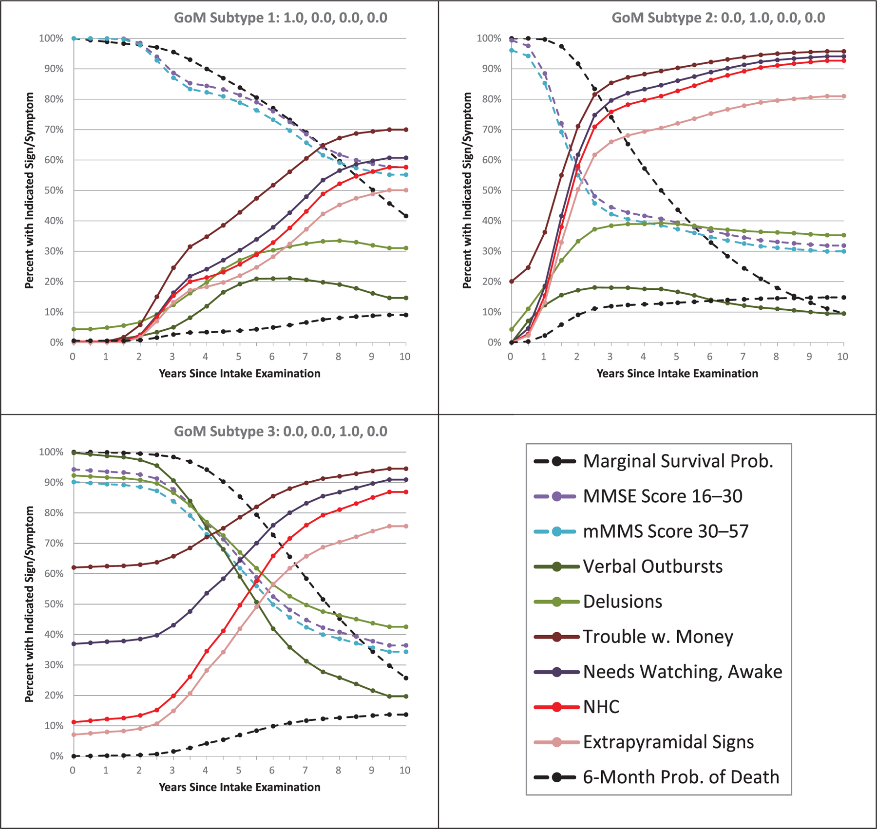
Marginal survival probabilities and conditional probabilities of death within 6 months, given survival to the respective visits, and corresponding conditional prevalence probabilities for need for high-level care (NHC) and six clinical signs/symptoms spanning six measurement domains in Table 1—for pure grade of membership (GoM) subtypes 1 through 3, respectively. Differences between the panels at time 0 reflect variation in initial presentations at the baseline visit. Differences between the panels in patterns of change over time reflect heterogeneity in disease progression. The NHC variable derives from the unaltered Dependence Scale without the upcoding for consistency with the Cox model in Figure 2

Figure 3 graphically illustrates how the L-GoM model incorporates changes in multiple variables over time, thus creating a full model of disease progression over correlated measurement domains. Differences in initial GoM scores are associated with marked differences in patterns of change over time across the various clinical features. Survival probabilities decline most rapidly in subtype 2. Also, there are more rapid declines in MMSE scores and increases in NHC in subtype 2 relative to subtypes 1 and 3. While subtype 3 is more debilitated than subtype 2 at time 0, it actually has more benign progression—further supporting the clinical relevance of the L-GoM model.

Table S.2 in supporting information displays the RMSE calculated by comparing the estimated probabilities in Figure 3 with the corresponding observed probabilities in the Predictors 2 study. The table shows that the L-GoM model provides a good representation of AD progression across the six measurement domains considered in Figure 3.

4 |. DISCUSSION

AD is heterogeneous, with multiple underlying pathologic processes. The course of the disease also varies widely across patients, most likely because of underlying biological and genetic heterogeneity. This makes accurate prediction of the course of AD challenging, though still important. On the clinical level, patients and their families want to know expected time to important disease endpoints. Clinical trials rely on differential progression in drug and placebo groups of cognitive and functional metrics, but do not take into account the inherent heterogeneity of disease course in patients included in their studies.

Here we present the validation and demonstration of our new model of AD progression, developed from the Predictors 2 data.¹ The model takes advantage of the multiple clinical features of the disease, as summarized in Table 1, and incorporates changes in all of these clinical features across 10 years, as summarized by data at each 6-month interval in that time period. We forward applied this model to a new data set—Predictors 1—and found that it quite accurately predicted mortality survival and NHC prevalence, based only on the initial visit assessment. We also developed new Cox models, similar to those in our prior article,⁹ that were specifically tailored to the two outcomes considered here, and that also showed very good predictive accuracy and provided a visual metric for assessing the L-GoM predictions, thereby supplementing the statistical testing.

Several advantages of the L-GoM model over the Cox model are apparent. While the L-GoM model incorporates all clinical variables, separate, independent Cox models need to be calculated for each clinical feature. Also, features whose prevalences are reversible are difficult to analyze with the Cox model but present no problem for the L-GoM model. For example, delusions increase over time in subtypes 1 and 2 while they decrease in subtype 3. Finally, Figure 3 illustrates how the L-GoM model describes changes in prevalence over time, for example, the prevalence of the need to be watched when awake at home, so it is suitable for fine-grained modeling of disease progression as opposed to simply calculating time to a specific endpoint.

To place L-GoM in context, we refer the reader to two recent reviews of existing AD models.^13,14 Green et al.¹³ identified 10 general modeling approaches from among 42 studies, with L-GoM¹⁵ constituting its own separate latent structure approach. Melis et al.¹⁴ identified 13 modeling approaches, characterizing our latest implementation of L-GoM¹ as “one of the few exercises to build a prognostic model for dementia progression.” AD modeling approaches generally try to predict the probability of some future clinical outcome based on currently observed clinical characteristics; they typically specify the logarithm (Poisson regression), logit (logistic regression), complementary log-log transform (Cox regression), or other nonlinear transformation of subject-specific outcome probabilities as linear functions of selected covariates (clinical signs/symptoms). L-GoM, as described in the Methods section, is distinguished as the only modeling approach that sidesteps the need for such nonlinear transformations by using linear functions of the derived latent scores to directly model the subject-specific outcome probabilities.

The recruitment criteria for the two Predictors studies are very similar to those used for many studies of mild to moderate AD. The cohorts are similar to other clinic based mild AD cohorts with respect to baseline characteristics.¹⁶ Their baseline characteristics and median survival are within the broad range seen in reviews of mild to moderate AD, though the broadness of the observed median survival suggests there is no single “representative” AD cohort.^17,18 Recruitment across three different AD centers also helps increase generalizability. However, the model requires further validation in additional samples. For example, the two cohorts were almost all White, non-Hispanic, well-educated AD patients selected through a nonrandom referral process into three specific AD research centers. This may limit generalizability to more diverse populations. We are currently conducting another validation study in a community-based, minority population.¹⁹ In addition, the validation covered only two of many possible endpoints, albeit two endpoints that are likely to be stable across study populations; this should be sufficient to validate the transition matrices used to generate the 6-month visit-specific GoM scores for each subject, thus increasing our confidence in accurate prediction for other clinical features in the model. Still, future validation analyses should address more of the included clinical features. While multiple clinical features are used to estimate a patient’s GoM status, many, such as mental and functional status, are typically ascertained by clinicians. In addition, it may be sufficient to obtain a subset of the measures so long as at least some information is provided for key domains of the model. The GoM score estimation can proceed with missing data without having to assume any specific values for the missing covariates (see supporting information).

Our earlier Cox-based prediction model⁹ was criticized because it included only patients who were ascertained with mild AD.²⁰ The critique was that the model would be more representative of the wider AD population if the data used to develop the model also included patients with moderate or severe levels of AD severity. While this critique has merit for Cox-based prediction models estimated from data from precisely one exam, that is, the initial visit, this critique does not hold for the L-GoM model estimated from all available data from recruitment at mild AD through as long as possible until death—thus representing all levels of AD severity.

Our L-GoM validation used data only from the initial visit in Predictors 1 to cover the important common case of patients presenting to clinicians with initially mild signs/symptoms of AD; this restriction also facilitated comparison with Cox-based prediction models. The model could also be applied to patients with moderate or severe disease at their initial visit, but we did not address that application here because neither Predictors 1 nor Predictors 2 had recruited such patients.

We also considered how our overall approach to development of the L-GoM model meets the five validation criteria proposed by Eddy et al.²¹: (1) L-GoM’s face validity derives from the usefulness of individual prognostication of the form displayed in Figure 3, (2) L-GoM’s internal validity derives from our double programming of the underlying calculations and verification that model parameters satisfy established conditions,²² (3) L-GoM’s cross validity derives from the comparisons with the Cox model in the present article, (4) L-GoM’s external validity derives from the present application of the Predictors 2 version of the model to the Predictors 1 data, and (5) L-GoM’s predictive validity is currently being evaluated in ongoing applications to the Predictors 3 and other data.

Eddy et al.²¹ also proposed two criteria for transparency: (1) documentation of the technical details of L-GoM was presented in Stallard et al.¹ and Stallard and Sloan²² and (2) non-technical documentation was presented herein and in Stallard et al.¹ We aimed for high levels of transparency by making the complete model readily available to readers in an accessible form. All parameters needed to apply the L-GoM model are contained in the supplementary Appendix to Stallard et al.,¹ with the smoothed transition matrices recommended for out-of-sample application provided in this article’s supporting information, which also provides simple fixed-point equations for GoM score estimation that can be readily implemented in Excel for individual prognostication using available covariates.

The L-GoM model can be used to estimate the future prevalence of any of the incorporated disease features and derivatively to estimate the durations of specific care needs and their associated ongoing and lifetime economic costs. Procedures for the analysis of the durations of specific care needs were presented in Stallard et al.¹ Compatible procedures for the analysis of Medicare, Medicaid, and long-term care costs of AD patients within the L-GoM framework were presented in Stallard et al.²³ and Stallard and Sloan;²² these procedures should be generally applicable in future work on the economic impact of AD using the L-GoM approach.

This aticle represents the first external validation and associated demonstration of our new L-GoM model. The model has great potential. We are developing a “calculator” to allow a doctor, patient, or family member to enter the clinical data available to them to generate customized predictions for the patient. As suggested by Figure 3, such a calculator can be extended to include multiple cognitive, functional, or psychiatric endpoints. More extensive use of the model will require “cross-walking” from the specific clinical measures used here to others often used in the field. Fortunately, the L-GoM model is very tolerant of missing data, so accurate predictions can be made even with limited data.²⁴ The ability of the L-GoM model to generate an expected time course of common metrics used in clinical trials offers great potential for study evaluation. Because the model incorporates multiple clinical measures, it can capture heterogeneity across subjects included in clinical trials even if they are similar in standard entry criteria based on MMSE scores or Clinical Dementia Rating scales. Thus, the GoM status at baseline could be used to check and improve randomization. Furthermore, if L-GoM predictions are accurate for the placebo group, then individual deviations from the predicted course in patients on experimental drugs could indicate a drug effect. Finally, the GoM status incorporates numerous time-varying clinical features of the disease into a single metric. This makes it a useful phenotype for genetic analyses, and for exploring the pathologic basis for the heterogeneity of AD.

HIGHLIGHTS.

• We validate a model of the progression of Alzheimer’s disease (AD).

• The model incorporates multiple clinical features across the entire disease process.

• The model accurately predicts time to mortality and dependency in an external population.

• We demonstrate the model’s utility in projecting changes in key clinical domains.

• The model is an important tool for patients, clinicians, clinical trialists, and other researchers.

RESEARCH IN CONTEXT.

1. Systematic Review:

The authors reviewed the literature using traditional published sources. There has been limited success in the development of comprehensive models of the progression of Alzheimer’s disease (AD) in heterogeneous longitudinally followed patient populations.

2. Interpretation:

We validated a comprehensive model of AD progression in an external data set. A novel feature of this model is that its inputs incorporate a wide range of disease features that are relevant to persons with AD and their caregivers. Model predictions of two representative outcomes—mortality and dependency—accurately reproduced the observed values, thereby confirming the validity of the underlying model. We then demonstrated how the model simultaneously describes inter-related change over time in multiple clinical features.

3. Future Directions:

This model of AD progression will allow prediction of the course of multiple disease features for individual patients or groups of patients, aid in interpreting clinical trial outcomes, and serve as a novel phenotype for exploration of the neuropathologic and genetic basis of heterogeneity in AD.

REFERENCES

- 1.Stallard E, Kinosian B, Stern Y. Personalized predictive modeling for patients with Alzheimer’s disease using an extension of Sullivan’s life table model. Alzheimers Res Ther. 2017;9:75. [DOI] [PMC free article] [PubMed] [Google Scholar]
- 2.Cosentino S, Scarmeas N, Helzner E, et al. APOE epsilon 4 allele predicts faster cognitive decline in mild Alzheimer disease. Neurology. 2008;70:1842–1849. [DOI] [PMC free article] [PubMed] [Google Scholar]
- 3.Stern Y, Folstein M, Albert M, et al. Multicenter study of predictors of disease course in Alzheimer disease (the “Predictors Study”). I. Study design, cohort description, and intersite comparisons. Alzheimer Dis Assoc Disord. 1993;7:3–21. [DOI] [PubMed] [Google Scholar]
- 4.Stern Y, Albert SM, Sano M, et al. Assessing patient dependence in Alzheimer’s disease. J Gerontol. 1994;49:M216–M22. [DOI] [PubMed] [Google Scholar]
- 5.McKhann G, Drachman D, Folstein M, Katzman R, Price D, Stadlan EM. Clinical diagnosis of Alzheimer’s disease: report of the NINCDS-ADRDA Work Group under the auspices of Department of Health and Human Services Task Force on Alzheimer’s Disease. Neurology. 1984;34:939–944. [DOI] [PubMed] [Google Scholar]
- 6.McKhann GM, Knopman DS, Chertkow H, et al. The diagnosis of dementia due to Alzheimer’s disease: recommendations from the National Institute on Aging-Alzheimer’s Association workgroups on diagnostic guidelines for Alzheimer’s disease. Alzheimers Dement. 2011;7:263–269. [DOI] [PMC free article] [PubMed] [Google Scholar]
- 7.Mayeux R, Stern Y, Rosen J, Leventhal J. Depression, intellectual impairment and Parkinson’s disease. Neurology. 1981;31:645–650. [DOI] [PubMed] [Google Scholar]
- 8.Stern Y, Sano M, Paulson J, Mayeux R. Modified mini-mental state examination: validity and reliability. Neurology. 1987;37(Suppl 1):179.3808297 [Google Scholar]
- 9.Stern Y, Tang MX, Albert MS, et al. Predicting time to nursing home care and death in individuals with Alzheimer disease. J Am Med Assoc. 1997;277:806–812. [PubMed] [Google Scholar]
- 10.Nair VN. Confidence bands for survival functions with censored data: a comparative study. Technometrics. 1984;26:265–275. [Google Scholar]
- 11.Kaplan EL, Meier P. Nonparametric estimatiion from incomplete observations. J Am Stat Assoc. 1958;53:457–481. [Google Scholar]
- 12.Agresti A, Coull BA. Approximate is better than “Exact” for interval estimation of binomial proportions. Am Stat. 1998;52:119–126. [Google Scholar]
- 13.Green C, Shearer J, Ritchie CW, Zajicek JP. Model-based economic evaluation in Alzheimer’s disease: a review of the methods available to model Alzheimer’s disease progression. Value Health. 2011;14:621–630. [DOI] [PubMed] [Google Scholar]
- 14.Melis RJF, Haaksma ML, Muniz-Terrera G. Understanding and predicting the longitudinal course of dementia. Curr Opin Psychiatry. 2019;32:123–129. [DOI] [PMC free article] [PubMed] [Google Scholar]
- 15.Kinosian BP, Stallard E, Lee JH, Woodbury MA, Zbrozek AS, Glick HA. Predicting 10-year care requirements for older people with suspected Alzheimer’s disease. J Am Geriatr Soc. 2000;48:631–638. [DOI] [PubMed] [Google Scholar]
- 16.Waring SC, Doody RS, Pavlik VN, Massman PJ, Chan W. Survival among patients with dementia from a large multi-ethnic population. Alzheimer Dis Assoc Disord. 2005;19:178–183. [DOI] [PubMed] [Google Scholar]
- 17.Brodaty H, Seeher K, Gibson L. Dementia time to death: a systematic literature review on survival time and years of life lost in people with dementia. Int Psychogeriatr. 2012;24:1034–1045. [DOI] [PubMed] [Google Scholar]
- 18.Todd S, Barr S, Roberts M, Passmore AP. Survival in dementia and predictors of mortality: a review. Int J Geriatr Psychiatry. 2013;28:1109–1124. [DOI] [PubMed] [Google Scholar]
- 19.Stern Y, Gu Y, Cosentino S, Azar M, Lawless S, Tatarina O. The Predictors study: development and baseline characteristics of the Predictors 3 cohort. Alzheimers Dement. 2017;13:20–27. [DOI] [PMC free article] [PubMed] [Google Scholar]
- 20.Rive B, Le Reun C, Grishchenko M, et al. Predicting time to full-time care in AD: a new model. J Med Econ. 2010;13:362–370. [DOI] [PubMed] [Google Scholar]
- 21.Eddy DM, Hollingworth W, Caro JJ, et al. Model transparency and validation: a report of the ISPOR-SMDM Modeling Good Research Practices Task Force–7. Value Health. 2012;15:843–850. [DOI] [PubMed] [Google Scholar]
- 22.Stallard E, Sloan F. Analysis of the natural history of dementia using longitudinal grade of membership models. In: Yashin AI, Stallard E, Land KC, eds. Biodemography of Aging: Determinants of Healthy Life Span and Longevity. New York: Springer; 2016. [Google Scholar]
- 23.Stallard E, Kinosian B, Zbrozek AS, Yashin AI, Glick HA, Stern Y. Estimation and validation of a multiattribute model of Alzheimer disease progression. Med Decis Making. 2010;30:625–638. [DOI] [PMC free article] [PubMed] [Google Scholar]
- 24.Razlighi QR, Stallard E, Brandt J, et al. A new algorithm for predicting time to disease endpoints in Alzheimer’s disease patients. J Alzheimers Dis. 2014;38:661–668. [DOI] [PMC free article] [PubMed] [Google Scholar]
- 25.Bianchi M, Boyle M, Hollingsworth D. A comparison of methods for trend estimation. Appl Econ Lett. 1999;6:103–109. [Google Scholar]
- 26.Devanand DP, Miller L, Richards M, et al. The Columbia University Scale for Psychopathology in Alzheimer’s disease. Arch Neurol. 1992;49:371–376. [DOI] [PubMed] [Google Scholar]
- 27.Folstein MF, Folstein SE, McHugh PR. Mini-mental State’: a practical method for grading the cognitive state of patients for the clinician. J Psychiatr Res. 1975;12:189–198. [DOI] [PubMed] [Google Scholar]
- 28.Blessed G, Tomlinson BE, Roth M. The association between quantitative measures of dementia and of senile change in the cerebral grey matter of elderly subjects. Br J Psychiatry. 1968;114:797–811. [DOI] [PubMed] [Google Scholar]
- 29.Fahn S, Marsden C, Calne D, Fahn S, Marsden C, Calne D. Recent Developments in Parkinson’s disease. Florham Park, N.J: Macmillan Healthcare Information; 1987. [Google Scholar]
- 30.Van Dyk K, Towns S, Tatarina O, et al. Assessing fluctuating cognition in dementia diagnosis: interrater reliability of the clinician assessment of fluctuation. Am J Alzheimers Dis Other Demen. 2016;31(2):137–143. [DOI] [PMC free article] [PubMed] [Google Scholar]
- 31.Wilks SS. The large-sample distribution of the likelihood ratio for testing composite hypotheses. Ann Math Statist. 1938;9:60–62. [Google Scholar]
Associated Data
This section collects any data citations, data availability statements, or supplementary materials included in this article.