

Abstract
Stable neural function requires an energy supply that can meet the intense episodic power demands of neuronal activity. Neurons have presumably optimized the volume of their bioenergetic machinery to ensure these power demands are met, but the relationship between presynaptic power demands and the volume available to the bioenergetic machinery has never been quantified. Here, we estimated the power demands of six motor nerve terminals in female Drosophila larvae through direct measurements of neurotransmitter release and Ca2+ entry, and via theoretical estimates of Na+ entry and power demands at rest. Electron microscopy revealed that terminals with the highest power demands contained the greatest volume of mitochondria, indicating that mitochondria are allocated according to presynaptic power demands. In addition, terminals with the greatest power demand-to-volume ratio (∼66 nmol·min−1·µl−1) harbor the largest mitochondria packed at the greatest density. If we assume sequential and complete oxidation of glucose by glycolysis and oxidative phosphorylation, then these mitochondria are required to produce ATP at a rate of 52 nmol·min−1·µl−1 at rest, rising to 963 during activity. Glycolysis would contribute ATP at 0.24 nmol·min−1·µl−1 of cytosol at rest, rising to 4.36 during activity. These data provide a quantitative framework for presynaptic bioenergetics in situ, and reveal that, beyond an immediate capacity to accelerate ATP output from glycolysis and oxidative phosphorylation, over longer time periods presynaptic terminals optimize mitochondrial volume and density to meet power demand.
SIGNIFICANCE STATEMENT The remarkable energy demands of the brain are supported by the complete oxidation of its fuel but debate continues regarding a division of labor between glycolysis and oxidative phosphorylation across different cell types. Here, we exploit the neuromuscular synapse, a model for studying neurophysiology, to elucidate fundamental aspects of neuronal energy metabolism that ultimately constrain rates of neural processing. We quantified energy production rates required to sustain activity at individual nerve terminals and compared these with the volume capable of oxidative phosphorylation (mitochondria) and glycolysis (cytosol). We find strong support for oxidative phosphorylation playing a primary role in presynaptic terminals and provide the first in vivo estimates of energy production rates per unit volume of presynaptic mitochondria and cytosol.
Keywords: calcium, electron microscopy, energy, mitochondria, oxidative, presynaptic
Introduction
Neurons are highly specialized in form and function. A facet of their specialization is a high power demand (rate of ATP consumption), which can be both highly localized and especially episodic (Le Masson et al., 2014; Rangaraju et al., 2014; Pathak et al., 2015; Li et al., 2020). The bioenergetic solutions that arose to meet these demands had to be housed in small volumes, as volume is a limited resource in complex nervous systems (Hasenstaub et al., 2010; Niven and Farris, 2012). Therefore, the bioenergetic design we see today represents a drive toward minimization to conserve resources, including volume, offset by a drive to meet power demands, in a system in which power failure in any number of circuits could be fatal. Integral to this bioenergetic design is a reliance on mitochondria, which represents both a key to the evolution of complex nervous systems and the weak link in many neurologic conditions (Devine and Kittler, 2018). Surprisingly, then, our understanding of this design is poor, partly because of a lack of data that quantifies subcellular power demands relative to the volume of bioenergetic machinery meeting those demands.
The bioenergetic machinery of a neuron can increase its output many-fold (Blomstrand et al., 1997; Walter et al., 1999) so that a given power demand might be satisfied by a small investment in machinery with output maximized, or, a large investment in machinery that idles. Correlates of elevated activity, such as elevations in Ca2+ levels, or ADP/ATP ratios, will stimulate the bioenergetic machinery, thus matching power supply to demand. For instance, neuronal oxidative phosphorylation (Ox Phos) accelerates within seconds of a burst of activity (Chouhan et al., 2012; Ashrafi et al., 2020), as does glycolysis (Díaz-García et al., 2017, 2021) and glucose uptake (Ashrafi et al., 2017). However, a limit will be reached, beyond which the bioenergetic machinery is unable to elevate output. A sustained elevation in Ox Phos is associated with elevated oxidative stress and with neurodegenerative disease (Pacelli et al., 2015), in which case neurons might be expected to accumulate mitochondria to an extent that minimizes the risk of needing to sustain elevated levels of Ox Phos. Similarly, there are limitations to accelerating glycolysis because of its dependence on NAD+ and the negative feedback from the acidic environment it creates (Erecińska et al., 1995; Yellen, 2018). Therefore, presynaptic terminals face constraints with regard to their mix of glycolytic and Ox Phos machineries and their total volume.
Numerous studies have demonstrated that levels of cytochrome c oxidase or mitochondrial volume correlate with measures of activity such as firing rate, active zone number or cumulative area, and synaptic vesicle (SV) number (Kageyama and Wong-Riley, 1982; Wong-Riley, 1989; Gulyás et al., 2006; Ivannikov et al., 2013; Rollenhagen et al., 2015, 2018; Buckmaster et al., 2016; Cserep et al., 2018; Yakoubi et al., 2018; Thomas et al., 2019). However, individual measures of activity can be poor predictors of power demand, as estimates of the latter require analyses of many parameters of subcellular form and function. Yet only through obtaining power demand estimates can we make a meaningful assessment of the volume apportioned to mitochondria, and only after power demand and mitochondrial volume are normalized to terminal volume can inferences be made about the relative contribution of Ox Phos and glycolysis. Here, we quantified the power demand of six nerve terminals that stereotypically innervate muscles of the Drosophila larva. Electron microscopy (EM) revealed that terminals with the highest power demand contained mitochondria with the greatest aggregate volume, density and individual size, providing for the first quantitative estimates of the power demands placed on presynaptic mitochondria.
Materials and Methods
Fly stocks
Drosophila stocks were raised at 24°C on standard medium [Bloomington Drosophila Stock Center (BDSC) recipe]. Measurements were performed on female third-instar larvae of a w1118 isogenized strain. Bloomington Drosophila Stock Center (Bloomington, IN) provided the following fly lines: UAS-mt8-GFP (stock #8443); UAS-myristoylated-tdTomato (stock #32222) and nSyb-GAL4 (stock #51635).
Solutions and chemicals
Larvae were dissected in Schneider's insect medium from Thermo Fischer (catalog #21720024) and physiological experiments were conducted in HL6 saline solution (Macleod et al., 2002). Chemicals were purchased from Sigma-Aldrich except where noted: 1.0 m CaCl2 Honeywell Fluka (catalog #21114-1L); 1.0 m MgCl2 Honeywell Fluka (catalog #63020-1L); rhod dextran, potassium salt, 10,000 MW, anionic (high-affinity version) Invitrogen (catalog #R34676, lot #1884364); Alexa Fluor 647 dextran, 10,000 MW, anionic, fixable Invitrogen (catalog #D22914).
Immunohistochemistry
Immunohistochemistry was conducted as described previously by Lu et al. (2016). Larvae were dissected in chilled Schneider's insect medium on Sylgard plates and rinsed three times with chilled HL6 (0 mm Ca2+ and 15 mm Mg2+). Preparations were then fixed with Bouin's solution (Sigma-Aldrich, catalog #HT10132) for 1 min at room temperature (RT; 23°C) and rinsed with PBS (pH 7.1; 4 × 10 min). After a rinse in PBS, the preparations were permeabilized with PBS-T (PBS containing 1% Triton X-100) for 1 h (4 × 15 min), then incubated for 30 min in a blocking solution [PBS containing 2% BSA, 5% goat serum (Sigma-Aldrich, catalog #G9023), 1% Triton X-100]. After blocking, preparations were incubated with primary antibodies (diluted with blocking solution) overnight at 4°C: mouse anti-Bruchpilot (1:200, nc82, supernatant; Developmental Studies Hybridoma Bank) and rabbit anti-Discs Large (DLG; 1:20,000; a gift from Benjamin Eaton). After incubation, preparations were washed with PBS-T for 1 h (4 × 15 min), and then incubated with fluorophore-conjugated secondary antibodies and the Cy3-conjugated goat anti-horse radish peroxidase (HRP: 1:600) for 1 h in darkness at RT: goat anti-mouse AF488 (1:400); donkey anti-rabbit Cy5 (1:200). Preparations were finally washed with PBS-T for 1 h (4 × 15 min), mounted on glass slides with antifade reagent (SlowFade Gold, catalog #S36937, Invitrogen) and covered with 0.16–0.19-mm glass cover-slips (Corning, catalog #2870-22).
Series of images were collected through the entire depth of each terminal on muscle fibers #6, #13, and #12 with an Olympus FV1000 confocal microscope with a 60 × 1.42 NA oil objective. Lasers (635, 543, and 488 nm) were used sequentially and emission filters were optimized for Cy5, Cy3, and AF488, respectively. No bleed-through from the other channels could be detected when imaging preparations incubated with single fluorophore-conjugated secondary antibody. Pinhole size was optimized with one value for all three imaging channels (115 µm, close to 1 Airy unit). Images were digitized at 10.6 pixels/µm in the X-Y plane, with a step depth (Z) of 0.2 µm.12-bit image stacks were collected, and raw data were output to ImageJ [Fiji (fiji.sc; ImageJ)] for analysis. DLG positive image stacks were used to distinguish different terminal types. Boutons of type-Ib terminals were distinguished from those of type-Is terminals by their larger size and denser DLG- positive subsynaptic reticulum (SSR). The “TrakEM2” plugin was used to quantify total nerve terminal volume and surface area.
The image in Figure 1B was acquired and assembled specifically to show all terminals relative to each other, which required four fields of view to be stitched together. The acquisition of these image differed from the images collected for quantification described above, as did some of the antibodies. A Nikon A1R confocal microscope was used with an Olympus 100 × 1.30 NA oil objective. Images were digitized at 8.4 pixels/µm in the X-Y plane. Antibodies: goat α-mouse AF555 with nc82 (1:24), donkey α-rabbit AF647 with α-DLG (1:4200), and, goat anti-HRP conjugated with AF488 (1:212).
Figure 1.

Drosophila larval motor neuron (MN) terminals are morphologically distinct. A, Diagrams showing a transverse section through a third-instar Drosophila larva, the location of the body-wall muscle fibers of interest and their stereotypical innervation by four glutamatergic MN axons (MN6/7-Ib, green; MN13-Ib, blue; MN12-Ib, pink; MNSNb/d-Is, red). B, A confocal micrograph of two MN terminals on each of muscle fibers #7, #6, #13, and #12, revealed through immunohistochemical labeling of the plasma membrane (blue; αHRP), active zones (magenta; αBrp, Nc82), and subsynaptic reticulum (SSR) of the muscle (green; αDLG). Each muscle fiber runs top-to-bottom on the image, as indicated by the dotted lines. Each colored circle indicates the color key used to identify the terminals on muscle fibers #6, #13, and #12 throughout the manuscript. C, D, Detail from the region bounded by corners in B. C, Channels separated according to antibody and fluorophore, as described in B. D, Channels separated as in C, but each rendered in an inverted grayscale to accentuate contrast. E, F, The average volume and surface area of the six glutamatergic terminals on muscle fibers #6, #13, and #12. Inset, Number of terminals measured, each on a separate larva (N); applies to both E, F. Two-way ANOVA with Tukey's HSD tests. Terminal volume (E): terminal type factor: p < 0.001, F(1,28) = 100.9; muscle identity factor: p = 0.237, F(2,28) = 1.5; factor interaction: p = 0.437, F(2,28) = 0.85. Terminal surface area (F): terminal factor: p < 0.001, F(1,28) = 72.3; muscle factor: p = 0.518, F(2,28) = 0.67; interaction: p = 0.877, F(2,28) = 0.13. Data and statistics are reported in Extended Data Table 1-1. All groups compared, but only those post hoc tests revealing significant differences are delineated (•p < 0.05, ••p < 0.01, •••p < 0.001). Box plots show mean (dotted line) and median values, with 25–75% boxes and 5–95% whiskers.
Electron microscopy
Third-instar larvae were fillet-dissected from a dorsal midline incision, prepared for EM as previously reported (Atwood et al., 1993), and sections cut serially at 100 nm (Lu et al., 2016). Image series collected at a magnification of 11,500 were assembled online as montages using software (Micrograph, Gatan Inc.) and then registered in vertical stacks using the TrakEM2 plugin for Fiji (https://imagej.net/TrakEM2; Cardona et al., 2012). Motor neuron (MN) terminals were reconstructed in three dimensions using additional software (Reconstruct; Fiala, 2005). The volumes of cytosol and mitochondria in motor axon terminals were measured using the TrakEM2 plugin for ImageJ (https://imagej.net/TrakEM2). Profiles of selected terminals were examined in each section, mitochondria labeled, and their profile areas selected from the sections and compiled with section thickness. In this way, the volumes of both the entire profile and for all mitochondria could be computed for each terminal. Mitochondria were counted and their averaged individual sizes estimated by dividing summed mitochondrial volume by the number of mitochondria in the terminal. A systematic difference in average SV outer diameter between terminal types is well established (Karunanithi et al., 2002) and we used this categorical difference to identify terminal type in EM micrographs. SV diameters were measured manually from micrographs using Fiji and we arrived at diameter estimates based on measurements at multiple boutons at each of 5 terminal pairs on muscle fiber #6 (Is: 43.75 ± 0.29; Ib: 33.39 ± 0.18; N = 5, SEM), that is generally consistent with a previous report (Karunanithi et al., 2002; Is, 45.0 nm; Ib, 38.5 nm).
To estimate glycolytic capable volume (cytosol) we subtracted the volume occupied by mitochondria and SVs from the terminal volume. The method used to calculate total mitochondrial volume cannot be used to calculate total SV volume, however, because SV diameters were less than the thickness of our EM sections (∼100 nm) introducing a stereological problem (Kim et al., 2000). The volume occupied by SVs was therefore estimated as follows: all SVs were counted in a series of 18 sections through a MNSNb/d-Is terminal on muscle fiber #6, and 41 sections through a MN6-Ib terminal. The type-Is boutons contained 3542 SVs in 4.24 µm3, while type-Ib boutons contained 46,952 SVs in 26.58 µm3, yielding numerical densities of 835 and 1766 SVs/µm3, respectively. Using Equation 14, we were then able to use estimates of SV numerical density, along with SV outer diameter estimates to calculate individual SV volume, and thereby calculate SV volume density. The proportion of each terminal occupied by SVs was estimated as 3.66% (Is) and 3.44% (Ib).
| (14) |
Cytosolic Density was calculated using Equation 15:
| (15) |
Cytosolic Volume was calculated using Equation 16:
| (16) |
An alternative estimate for glycolytic capacity might be generated from the summed surface area of internal membranes (SVs and inside plasma membrane), given that glycolytic components are known to associate with these membranes (Hinckelmann et al., 2016). Using data from above for terminals on muscle #6, and Extended Data Table 1-1, we calculated values of 697 µm2 (MNSNb/d-Is) and 2489 µm2 (MN6-Ib), which ironically delivered a similar proportion of internal membrane surface area between terminals (3.57) as cytosolic volume (280.4/83.1 µm3 = 3.37). Therefore, using Occam's razor, we defaulted to cytosol volume as the measure of glycolytic capacity.
Terminal morphology. Download Table 1-1, XLSX file (11.3KB, xlsx) .
Electrophysiology
All larvae were dissected in chilled Schneider's medium, as illustrated previously (Rossano and Macleod, 2007), then switched to HL6 saline (2 mm Ca2+ and 15 mm Mg2+) before electrophysiology. Current Clamp recordings were conducted simultaneously on two adjacent muscle fibers from muscles #6, #13, or #12 in abdominal segment four to identify the evoked response of either type-Ib or -Is MNs using the voltage threshold technique (Lu et al., 2016). Signals were detected, digitized and recorded using an Axoclamp 900A amplifier (Molecular Devices) connected to a 4/35 PowerLab (ADInstruments) and a PC running LabChart v8.0. Micropipettes were pulled from borosilicate capillary tubing (catalog #BF15086-10, Sutter Instruments) on a Flaming/Brown P-97 micropipette puller and filled with a 1:1 mixture of 3 m KCl and 3 m K-acetate. Once the evoked response was identified, muscle fibers were clamped to –60 mV via a two-electrode voltage clamp (TEVC). A 0.1 gain head-stage and ∼50 MΩ was used for voltage recording. A 1.0 gain head-stage and ∼15-MΩ micropipette was used for passing current. The identified MN was stimulated at its endogenous firing rate (EFR) for the duration of its duty cycle (DC) during recordings (Fig. 2B). Voltage deflections were <5 mV for EJCs as large as 100 nA. Only records from muscle fibers that maintained a resting membrane potential (RMP) of greater than −60 mV for muscle 6 and greater than −50 mV for muscles 13 and 12 were used. Recordings with action potential (AP) failure, or the recruitment of another MN (compound EJCs) were discarded. It is important to note that most (∼60%) recordings were discarded, as, unless axon thresholds were well separated (by chance alone) then it was unlikely that a record suitable for quantification could be obtained. The initial amplitude and degree of frequency facilitation appeared to be no different in those recordings that were discarded from those that were fully analyzed. MN13-Ib was the most difficult to isolate, e.g., three out of 139 larval preparations (Extended Data Table 2-1); ≥30 mEJPS were collected at each of 26, 12, and 10 muscle fibers (muscles #6, #13, and #12, respectively). Quantal content (QC; Fig. 2E) was calculated using Equation 17:
| (17) |
Figure 2.

Terminals are physiologically distinct, with different power demands for recycling and refilling synaptic vesicles (SVs). A, A diagram of a transverse section through muscle fibers #7, #6, #13, and #12 and their innervating motor neurons (MNs). Simultaneous current-clamp recordings in adjacent muscle fibers were used to identify which MN released neurotransmitter in response to an AP. A single muscle fiber was then voltage clamped with two electrodes to allow quantification of AP-evoked release. B, Sample electrophysiological traces showing EJCs, evoked from different MNs, as indicated. Release was evoked at the endogenous firing rate (EFR) (Hz) and for periods of time representing each MN's DC during peristaltic cycles of locomotion (1 per second). Recordings conducted in HL6 saline; 2 mm [Ca2+]o and 15 mm [Mg2+]o. C, Sample trace showing mEJCs recorded in muscle fiber #12. D, Plots of average EJC amplitude for each MN over the first peristaltic cycle (SEM shown). Arrows point to the mid-train EJC measured to quantify the physiological QC. Inset, Number of separate larvae (N) in which trains were evoked; applies to D–H. E, Plots of the average QC of each terminal, calculated by dividing the average physiological EJC amplitude by the average mEJC amplitude after mEJC amplitude is adjusted for terminal identity (see Materials and Methods for more details). F, Plots of the estimated number of glutamate molecules released after a single AP for each terminal (GluAP; Eq. 1). G, Plots of the estimated average amount of ATP spent to recycle and refill SVs after a single AP [E(GluAP); Eq. 2]. H, Quantification of the power demand for SV recycling and refilling for each terminal when active for a peristaltic cycle (1 s), as defined in D (PGlu; Eq. 3). Two-way ANOVAs applied in E–H. Data and statistics reported in Extended Data Table 2-1. The results of post hoc tests are only shown for power demand for SV recycling and refilling (H), where a two-way ANOVA was performed on ranks with Tukey's HSD tests. Terminal factor: p < 0.001, F(1,42) = 135.1; muscle factor: p = 0.038, F(2,42) = 3.5; interaction: p = 0.006, F(2,42) = 5.7. Only those post hoc tests revealing significant differences are delineated (•p < 0.05, ••p < 0.01, •••p < 0.001). Box plots (E–H) show mean (dotted line) and median, with 25–75% boxes and 5–95% whiskers.
Since the quantal size of type-Is is on average ∼50% larger than that of type-Ib mEJCs (Karunanithi et al., 2002; Pawlu et al., 2004; Dawson-Scully et al., 2007), a scaling factor was applied to mEJCs to accommodate the type-Is terminals giving rise to larger mEJCs. The QC of type-Is terminals was multiplied by 0.8 and the QC of type-Ib terminals was multiplied by 1.2 (Lu et al., 2016).
Terminal firing patterns and electrophysiology data. Download Table 2-1, XLSX file (13.4KB, xlsx) .
Ca2+ imaging for estimating Ca2+ entry
All larvae were dissected in chilled Schneider's media and forward-filled with a 10,000 MW dextran-conjugated Ca2+ indicator (rhod) and dextran-conjugated Ca2+ insensitive dye (AF647) in a constant ratio of ∼50:1 (4.76 mm rhod/0.10 mm AF647), as described previously (Macleod, 2012). Ca2+ imaging was performed under a water-immersion 100×/1.10 NA objective on a Nikon microscope (Eclipse FN1), fitted with an EMCCD camera (Andor Technology, iXonX3 DU897), running at 102.7 frames per second. The preparation was illuminated by a Lumencor Spectra X LED light source through a 550/15-nm excitation filter for rhod and 640/30-nm excitation filter for AF647. Emission was collected through a Nikon instruments filter wheel with filter cubes for rhod (FF562nm-Di03, 590/36-nm) and AF647 (Di89100bs, 705/72 nm). Filters and dichroic mirrors were obtained from Chroma Technology or Semrock. During rhod imaging, each preparation was stimulated via Master 8 Stimulator (AMPI) at 1 Hz for 10 s. The ten AP-evoked Ca2+ responses were aligned and averaged for each terminal.
Calibration
Fluorescence signals were converted to [Ca2+] using Equation 5 of Grynkiewicz et al. (1985). Values of Rmin were obtained in situ by incubating preparations in Ca2+-free HL6 with 1 mm EGTA and 100 mm BAPTA-AM (1% DMSO, 0.2% pluronic acid) for 20 min (catalog #B6769; Invitrogen). Values of Rmax were obtained in situ by incubating preparations in HL6 containing 10 mm Ca2+ and 100 μm ionomycin (catalog #I9657, Sigma) for 30 min (Chouhan et al., 2010). The KD value used for rhod dextran (1.754 μm) was determined in vitro by measuring its fluorescence relative to AF647 in a series of solutions with different levels of free Ca2+. The series was established by blending two solutions from a Ca2+ calibration kit (catalog #C3008MP; Invitrogen); a low Ca2+ solution (10 mm K2EGTA) and a high Ca2+ solution (10 mm CaEGTA). Both solutions contained 100 mm KCl and 30 mm MOPS, prepared in deionized water at pH 7.2. K+ concentrations were supplemented by adding ∼95 µl 1 m KCl (catalog #P3911, Sigma) to 2 ml to bring the osmolarlity to 340 mOsm (measured in a Vapro vapor-pressure osmometer, model 5520). Free Ca2+ levels were determined by reference to MaxChelator (https://somapp.ucdmc.ucdavis.edu/pharmacology/bers/maxchelator/).
Estimation of dye loading
Rhod loading was determined by dividing the fluorescence intensity of AF647 (co-loaded in constant ratio with rhod) in the center of a bouton by the fluorescence intensity of AF647 in a glass capillary filled with the rhod/AF647 mixture of known concentration. The same illumination and exposure settings used for calibration measurements were used for each experiment. As the diameter of a capillary will inevitably differ from the diameter of a bouton (and as bouton diameters will differ between terminals), we needed to correct for differences in path length, especially because we used wide-field optics were used. The procedure was as follows: immediately before the acquisition of Ca2+ indicator fluorescence transients, a series of images of AF647 fluorescence was acquired through the depth of the bouton. Close-to spherical boutons were selected where possible and we measured the average pixel intensity in a centrally positioned 3 × 3-pixel region of interest (ROI; 0.75 × 0.75 µm ROI). A measurement from the plane of focus with the maximum average pixel intensity was compared with a measurement from the glass capillary obtained similarly, after measurements from both boutons and capillary were corrected as described previously (Lu et al., 2016; their Appendix S2). Briefly, maximum fluorescence measurements were corrected according to the apparent z-dimension of the bouton (or capillary) to compensate for out-of-focus rhod or AF647 fluorescence that might have otherwise contributed to the intensity measurement.
Estimation of incremental Ca2+ binding ratio (K'B)
K'B was determined using Equation 18 (Eq. 4 of Helmchen et al., 1996):
| (18) |
where the Ca2+ dissociation constant (Kd) was determined in vitro for rhod-dextran (1.754 μm; described above), and where we determined the cytosolic concentration of rhod ([rhod]) in situ (described above) and [Ca2+]rest. The terminals were all loaded for similar periods; 6Ib: 278.4 ± 5.6 min; 6Is: 295.9 ± 11.1 min; 13Ιb: 280.9 ± 6.4 min; 13Is: 291.6 ± 13.2 min; 12Ib: 292.4 ± 10.4 min; 12Is: 301.2 ± 14.5 min, and values of [rhod] were calculated as 6Ib: 46.2 ± 8.6 μm; 6Is: 31.7 ± 6.1 µm; 13Ιb: 70.8 ± 13.7 µm; 13Is: 35.7 ± 6.8 µm; 12Ib: 65.8 ± 11.9 µm; and 12Is: 33.39 ± 8.5 µm SEM. Mean and SEM are reported for loading and concentration. As there was little to substantiate the difference in endogenous Ca2+ binding ratio (Ks) between terminals MN6Ib and MN6Is as previously reported (Lu et al., 2016), the average Ks of MN6Ib and MN6Is (48.35) was adopted for all terminals.
Estimating Na+ entry
Indirect estimates of total Na+ entry relied on the method used previously by Lu et al. (2016), as described in Results. APs were assumed to actively invade all terminals with a voltage displacement of 100 mV, although the magnitude of the AP has not been measured for Drosophila MN terminals.
Estimating nonsignaling power demands
Estimates of nonsignaling power demand were derived from O2 consumption rates (OCRs) from unstimulated rat brain slices (∼1 mm O2/min; Engl et al., 2017) scaled to the volume and plasma membrane area (surface to volume ratio) of Drosophila MN terminals. The application of this value to Drosophila MNs assumes that the density of Na+-permeant channels and carriers is similar between Drosophila MN terminals and rat hippocampal neuropil. An assumption is also made that the amount of protein/lipid synthesis, cytoskeleton turnover and membrane is uniform across MN terminals. While rat central nervous tissue at ∼37°C might represent a strained analogy for Drosophila MN terminals at RT, the measurements of Engl et al. (2017) probably represent the best controlled and quantified values for the various components of nonsignaling energy demands. To the extent that the systems diverge, any error will be pro-rated according to size and surface area of each terminal, which would be unlikely to result in any change in the proportion of total power estimated between terminals. Engl et al. (2017) estimated that processes occurring in the cytosol [cytoskeleton turnover (47%) and lipid/protein synthesis (18%)] consumed 65% of the oxygen at rest, while processes at the plasma membrane (Na+/K+ ATPase) consumed 50%. Reconciling these values as approximate fractions of a 1 mm/min OCR, cytosolic processes consume an estimated ∼0.6 mm/min (65%/115%), while plasma membrane processes consume an estimated ∼0.4 mm/min (50%/115%). The cytosol of MN6Ib, with a volume of 310 µm3, would be expected to consume 310 µm3/1 × 1015 µm3 × 0.6 mm O2/min = 1.86 × 10⁻¹³ mm O2/min [or 1.86 × 10⁻¹³ mm O2/min (where 1 × 1015 µm3 = 1 l)]. The rat hippocampal neuropil plasma membrane-to-volume ratio is 14 × 1015 µm2/l (Lehre and Danbolt, 1998; Rusakov and Kullmann, 1998) and so, if equivalent, MN6Ib, with a surface area of 568 µm2, would be expected to consume 568 µm2/14 × 1015 µm2/l × 0.4 mm O2/min = 1.62 × 10⁻¹⁴ mm O2/min at the plasma membrane at rest. To convert OCR to power (ATP/s), an assumption is made that the OCR reflects sequential and complete oxidation of glucose by glycolysis and oxidative phosphorylation. Under these conditions, and assuming a maximum P/O of 2.79 (moles of ATP generated per mole of [O] consumed; oxygen atoms; Mookerjee et al., 2017), the consumption of one oxygen molecule signals the net production of 2 × 2.79 = 5.58 ATP molecules, and so cytosolic and plasma membrane OCRs convert to 1.04 × 10⁷ and 9.09 × 10⁵ molecules ATP/s (1.73 × 10⁻¹⁴ and 1.51 × 10⁻¹⁵ mm ATP/s), respectively.
Statistical analysis and data presentation
Tests were performed using SigmaStat 3.5 and GraphPad software. For multiple comparisons, ANOVA was applied and an overall α of <0.05 was required to claim significance. When testing for differences between terminals, a two-way ANOVA was used because terminals are functionally differentiated between type (factor 1: type-Ib and -Is; Kurdyak et al., 1994; Chouhan et al., 2010; Lu et al., 2016), and between muscle fibers (factor 2: muscle fibers number 6, 13, and 12; Chouhan et al., 2012). ANOVAs were run on ranks when tests for data normalcy failed. Propagation of uncertainty theory (Farrance and Frenkel, 2012) was used to calculate variance of means based on uncertainty measurements (SEM) combined from different experiments. ANOVAs were run on raw data except in Figures 5A, 6H, where two-way ANOVAs with Tukey's multiple comparisons were run on means, SEM from propagated uncertainty, and N. Pearson product-moment correlation coefficient was calculated to test the strength and direction of associations, and as the data being examined passed tests for normalcy and equal variance, without data transformation, the ordinary-least-squares method was used to provide linear fits. For calcium imaging, measurements were assessed for outliers using the median absolute deviation (MAD; Leys et al., 2013), where an outlier was considered to be any value beyond 5 × MAD of the median.
Figure 5.

Type-Ib terminals consume more energy per unit volume during physiologic activity. A, Plots of the power demand during signaling (sum of PGlu, PCa2+, and PNa+), nonsignaling and total power demand (sum of signaling and nonsignaling power demands) for each terminal (see Materials and Methods). Error bars (SEM) were calculated according to propagation of uncertainty theory. Error may be underestimated as PGlu, PCa2+, and PNa+ may be correlated, yet covariance could not be estimated for each terminal. Inset shows detail of differences in nonsignaling power demand. Two-way ANOVAs applied with Tukey's HSD tests. Signaling (left): terminal factor: p < 0.001, F(1,23) = 1065; muscle factor: p < 0.001, F(2,23) = 20.5; interaction: p < 0.001, F(2,23) = 22.0. Nonsignaling (center): terminal factor: p < 0.001, F(1,23) = 112.6; muscle factor: p = 0.217, F(2,23) = 1.6; interaction: p = 0.440, F(2,23) = 0.8. Total (right): terminal: p < 0.001, F(1,23) = 1150; muscle: p < 0.001, F(2,23) = 21.4; interaction: p < 0.001, F(2,23) = 22.8. Only those post hoc tests revealing significant differences are delineated (•p < 0.05, ••p < 0.01, •••p < 0.001). B, Plots of nonsignaling demand and total power demand versus terminal volume. For each plot, Pearson's correlation coefficient indicated a significant correlation with terminal volume; nonsignaling: r = 1.00, p < 0.001; total: r = 0.99, p < 0.001. Data and statistics reported in Extended Data Tables 5-1, Tables 5-2.
Figure 6.
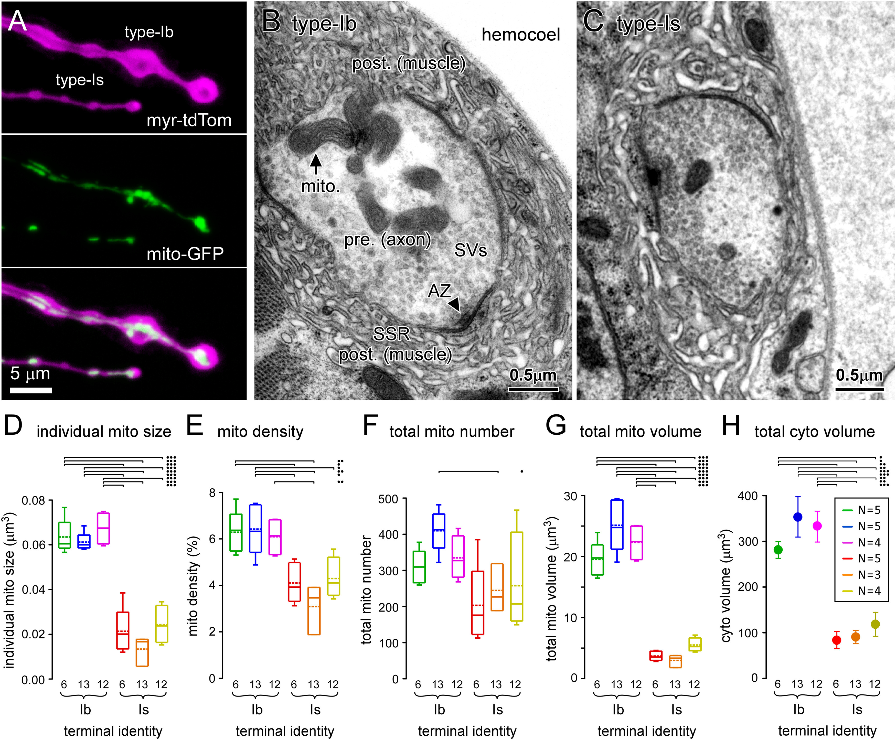
Terminals with the greatest power demands have the greatest mitochondrial size, density, number, and volume. A, Images of fluorescent proteins expressed in type-Ib and -Is terminal boutons on muscle fiber #13 (MN13-Ib and MNSNb/d-Is, respectively), using the nSyb MN driver, targeted to the PM (myristoylated tdTomato) and mitochondrial matrix (mt8-GFP). B, C, Transmission electron micrographs of 100-nm-thick sections through type-Ib and -Is terminal boutons on muscle fiber #6 (MN6/7-Ib and MNSNb/d-Is, respectively). D, Plot of the average individual mitochondrion size within each terminal. E, Plot of the average density of mitochondria in each terminal. F, Plot of the average number of mitochondria in each terminal, quantified using Equation 13. G, Plot of the average total mitochondrial volume occupying each terminal quantified using Equation 12. H, Plot of the average total cytosolic volume of each terminal quantified using Equation 16. Box plots (D–G) show mean (dotted line) and median, with 25–75% boxes and 5–95% whiskers. Error bars (SEM) were calculated according to propagation of uncertainty theory in G. The number (N) of reconstructed terminals (for D–H) is shown in inset in H. Two-way ANOVAs with Tukey's HSD tests applied in D–H. ANOVAs were performed on ranks in D, F. Individual mitochondrial size (D): terminal factor: p < 0.001, F(1,20) = 92.4; muscle factor: p = 0.093, F(2,20) = 2.7; interaction: p = 0.915, F(2,20) = 0.09. Mitochondrial density (E): terminal factor: p < 0.001, F(1,20) = 41.6; muscle factor: p = 0.573, F(2,20) = 0.57; interaction: p = 0.275, F(2,20) = 1.4. Total number of mitochondria (F): terminal: p = 0.002, F(1,20) = 12.5; muscle: p = 0.245, F(2,20) = 1.5; interaction: p = 0.580, F(2,20) = 0.56. Total mitochondrial volume (G): terminal factor: p < 0.001, F(1,20) = 292.6; muscle factor: p = 0.117, F(2,20) = 2.4; interaction: p = 0.059, F(2,20) = 3.3. Total cytosolic volume (H): terminal factor: p < 0.001, F(1,20) = 60.8; muscle factor: p = 0.383, F(2,20) = 1.0; interaction: p = 0.637, F(2,20) = 0.46. Only those post hoc tests revealing significant differences are delineated (•p < 0.05, ••p < 0.01, •••p < 0.001). Data and statistics reported in Extended Data Table 6-1.
Results
This study can be divided into four parts. First, we quantify the morphologic and physiological characteristics of six MN terminals formed by four different MNs innervating four muscle fibers. Second, we use a “bottom-up” approach to estimate the ATP requirements for a single AP for each terminal. We then calculate the ATP consumption rate (power demand) of each terminal during physiological activity, and at rest. Lastly, we quantify mitochondrial size, number, volume and density in each terminal, and compare these data with our estimates of power demand.
Drosophila MN terminals are morphologically and physiologically distinct
MN terminals in the body wall of Drosophila larvae provide an opportunity to quantify energy consumption rates (the power demand) of functionally differentiated terminals under physiological conditions. Four glutamatergic MNs innervate four muscle fibers (#7, #6, #13, and #12) in a stereotypical pattern (Fig. 1A; Hoang and Chiba, 2001). A terminal with large boutons [type-Ib (big)] can be found on each muscle fiber, and the terminals on muscles #6, #13, and #12 each arise from a different MN, while a terminal with small boutons [type-Is (small)] can also be found on each muscle fiber (Fig. 1B–D). Type-Is terminals, however, derive from a single MN. Immunofluorescence and confocal microscopic analysis revealed that type-Ib terminals have a substantially larger volume and surface area than type-Is terminals (Fig. 1E,F).
The EFRs are quite different between MNs and have been well characterized (Chouhan et al., 2010, 2012; Lu et al., 2016; Extended Data Table 2-1). The DC (the proportion of time that a MN fires during a peristaltic cycle) is also quite different between different MNs (Klose et al., 2005; Lu et al., 2016). MNs with type-Ib terminals fire at faster rates and for longer periods than the MN with type-Is terminals. Each MN was stimulated ex vivo, according to the pattern predicted for two consecutive contractions during unrestrained locomotion, and our electrophysiological recordings (Fig. 2B,C) revealed different extents of frequency facilitation, i.e., some facilitated while others depressed (Fig. 2D).
Power demands differ substantially between different MN terminals
We estimated both the signaling and nonsignaling (housekeeping) power demand (ATP/s) of different nerve terminals. We estimated signaling power demand using the “bottom-up” approach of Lu et al. (2016) through direct measurements of neurotransmitter release, calcium ion (Ca2+) entry, and theoretical estimates of sodium ion (Na+) entry. Nonsignaling power demand, also referred to as power demand at rest, was estimated by comparing the volume and surface area of each terminal with terminals in nervous tissue in which nonsignaling OCR has been measured previously (Engl et al., 2017).
Quantification of signaling power demands
The cost to recycle and refill SVs
The recycling and refilling of SVs with neurotransmitters consumes large amounts of ATP during neurotransmission (Rangaraju et al., 2014; Pathak et al., 2015; Sobieski et al., 2017). The number of SVs released can be estimated through electrophysiological measurements at the postsynaptic (muscle) membrane. For each terminal, we determined the QC (number of SVs exocytosing per AP) using a protocol adopted from Lu et al. (2016) that could determine whether evoked postsynaptic potentials were the result of release from a type-Ib or a type-Is terminal (Fig. 2A). To estimate the QC during locomotion, each MN was stimulated at its EFR (Fig. 2B), and the amplitude of an excitatory junction current (EJC) was measured half way through its DC (Fig. 2B,D, arrows). QC was then calculated by dividing the amplitude of this EJC by the average amplitude of miniature EJCs (mEJCs; Extended Data Table 2-1) once the mEJC amplitudes were adjusted for terminal type (see Materials and Methods). The number of glutamate molecules released in response to a single AP (GluAP) for each terminal was determined using Equation 1 (Fig. 2F):
| (1) |
where ε is the number of glutamate molecules in a SV, obtained from Lu et al. (2016; ε; Is: 9600; Ib: 6400).
To determine the energy required (E; ATP molecules), to recycle and refill SVs with glutamate after a single AP, Equation 2 was used (Fig. 2G):
| (2) |
where the estimated cost of exocytosis and endocytosis of a single SV is 410.5 ATP molecules, and it costs 2.67 ATP molecules to load a glutamate molecule into a SV (Attwell and Laughlin, 2001).
To determine the power demand (P; ATP/s) for SV recycling and refilling during physiological activity, Equation 3 was used, and type-Ib terminals were found to use ATP at a higher rate when recycling and refilling SVs than type-Is terminals (Fig. 2H).
| (3) |
where ⌈⌉ is the ceiling function (integer directly above), EFR × DC is the number of APs per DC, and FC is the duration of a full peristaltic cycle (1 s).
The cost of Ca2+ extrusion
The extrusion of Ca2+ is another major consumer of ATP during neurotransmission (Harris et al., 2012). In Drosophila MN terminals, Ca2+ extrusion is primarily mediated by the plasma membrane Ca2+-ATPase (PMCA; Lnenicka et al., 2006). For every one Ca2+ extruded, one ATP molecule is hydrolyzed (Attwell and Laughlin, 2001). To estimate the amount of ATP consumed to extrude cytosolic Ca2+ per AP, the total number of Ca2+ that enters each terminal during an AP (ΔCa2+total) was determined using Equation 4:
| (4) |
where Δ[Ca2+]total is the change in total Ca2+ (free + bound; mol/l), vol is the volume of the terminal (L), and AN is Avogadro's constant. The volume of each terminal was estimated from confocal microscopy images (see Materials and Methods; Fig. 1E). Δ[Ca2+]total was calculated using Equation 5:
| (5) |
where Δ[Ca2+]AP is the change in cytosolic-free Ca2+ concentration in response to a single AP, Ks is the endogenous Ca2+ binding ratio, and K'B is the incremental Ca2+ binding ratio for the exogenous Ca2+ buffer, rhod. Δ[Ca2+]AP was measured by microfluorimetry after forward-filling terminals with a mixture of Ca2+-sensitive fluorescent dye and a Ca2+-insensitive fluorescent dye in constant ratio (∼50:1; rhod dextran: AF647 dextran; Fig. 3A). A single value of Ks (48.35), derived from the values reported by Lu et al. (2016), was used for all terminal types. K'B was calculated as described in Materials and Methods (Extended Data Table 3-1). A single AP generally elicits a greater Δ[Ca2+]AP (Fig. 3B,C) and Δ[Ca2+]total (Fig. 3D) in type-Is terminals when compared with type-Ib. Consistently, the time integral of the Ca2+ transient, the product of Δ[Ca2+]AP and its time course of decay (τ; Fig. 3E), which is relatively independent of exogenous Ca2+ buffer loading, was also significantly higher for type-Is terminals when compared with type-Ib terminals (Fig. 3F). While type-Is terminals generally show a larger Δ[Ca2+]AP and Δ[Ca2+]total, type-Ib terminals have much larger volumes resulting in far greater values of ion influx (ΔCa2+total) after a single AP (Fig. 3G).
Figure 3.

Terminals differ greatly in their power demands for Ca2+ extrusion. A, Inverted grayscale images of fluorescence from type-Ib and -Is bouton terminals on muscle fiber #6. Terminals are filled with AF647-dextran [top; single frame collected at 10 frames per second (fps)] and rhod-dextran (middle and bottom; average of 10 frames collected at 10 fps). The motor nerves received 10 impulses at 1 Hz. The middle image shows average rhod fluorescence in the 98-ms interval before an impulse, and the bottom image shows the 98-ms period after an impulse. B, Traces revealing the transient increase in free Ca2+ ([Ca2+]AP) in response to single APs for each terminal. Each trace represents the average of 10 APs (Ca2+ transients) from a single terminal. [Ca2+] was estimated from an in situ calibration of rhod fluorescence relative to AF647 (see Materials and Methods). C, Plots of the average change in [Ca2+]AP (Δ[Ca2+]AP) estimated from ten synchronized stimuli at 1 Hz. D, Plots of the average change in total Ca2+ concentration (bound and unbound Ca2+) in response to a single AP (Δ[Ca2+]total; Eq. 5). E, Plots of average time course of decay of [Ca2+]AP transients for each terminal. F, Plots of average time integral (Δ[Ca2+]AP × τ; nM.s) for each terminal. G, Plots of total influx (number) of Ca2+ ions during a single AP [(ΔCa2+ total); Eq. 4]. H, The power demand for Ca2+ extrusion for each terminal when active for a peristaltic cycle (1 s), as shown in Figure 2D [(PCa2+); Eq. 7]. Inset, Number of terminals from different larvae, each a sample of 10 APs, as in B; applies to C–H. Two-way ANOVAs with Tukey's HSD tests applied in C–H. Δ[Ca2+]AP (C): terminal factor: p < 0.001, F(1,56) = 23.7; muscle factor: p = 0.166, F(2,56) = 1.9; interaction: p = 0.852, F(2,56) = 0.85. Δ[Ca2+]total/AP (D): terminal factor: p < 0.001, F(1,56) = 26.1; muscle factor: p = 0.118, F(2,56) = 2.2; interaction: p = 0.803, F(2,56) = 0.22. Time integral (F): terminal factor: p < 0.001, F(1,56) = 24.2; muscle factor: p = 0.013, F(2,56) = 4.7; interaction: p = 0.666, F(2,56) = 0.41. Ca2+ influx/AP (G): terminal factor: p < 0.001, F(1,56) = 30.4; muscle factor: p = 0.030, F(2,56) = 3.7; interaction: p = 0.556, F(2,56) = 0.59. The two-way ANOVA was performed on ranks for power demand of Ca2+ extrusion (H): terminal: p < 0.001, F(1,56) = 141.4; muscle: p = 0.108, F(2,56) = 2.3; interaction: p = 0.250, F(2,56) = 1.4. Only those post hoc tests revealing significant differences are delineated (•p < 0.05, ••p < 0.01, •••p < 0.001). Box plots (C–H) show mean (dotted line) and median, with 25–75% boxes and 5–95% whiskers. Data and statistics reported in Extended Data Table 3-1.
Calcium imaging. Download Table 3-1, XLSX file (12.8KB, xlsx) .
To calculate the total number of ATP molecules required to extrude Ca2+ for a single AP, Equation 6 was used:
| (6) |
To determine the power required (P; ATP/s), for Ca2+ extrusion during physiological activity, Equation 7 was used. Type-Ib terminals expend ATP at a faster rate when extruding cytosolic Ca2+ than do type-Is terminals (Fig. 3H).
| (7) |
The cost of Na+ extrusion
The reestablishment of plasma membrane Na+ and K+ gradients, subsequent to APs, is also a significant presynaptic cost associated with neurotransmission (Harris et al., 2012). In nerve terminals, Na+ is extruded primarily through the Na+/K+ antiporter (Attwell and Laughlin, 2001), and for every three Na+ ions that are extruded, one ATP molecule is hydrolyzed (Forgac and Chin, 1981). To estimate the amount of ATP required to extrude Na+, the total amount of Na+ that entered each terminal during an AP (Na+AP) must first be determined. Insofar as Drosophila MN terminals are surrounded by the SSR of the muscle cell, it is physically impossible to voltage clamp the presynaptic membrane to measure the amount of Na+ directly. An indirect estimate of the minimum amount of Na+ entering the entire terminal during an AP can be calculated using Equation 8:
| (8) |
where a charge (q; Coulombs) is needed to change the voltage (V; volts) across the capacitance (C; µF) of the presynaptic membrane by the amplitude of the AP (Carter and Bean, 2009). The inward Na+ current and outward K+ current underlying an AP of amplitude V are illustrated in Figure 4A. Values for V (0.1 V) and C (1 µF cm−2) were taken from Lu et al. (2016). Equation 9 was used to calculate the total number of Na+ ions that entered during an AP (Na+AP; Fig. 4B) assuming Na+ was solely responsible for the rising phase of the AP.
| (9) |
where the surface area of each nerve terminal was estimated from confocal microscopic examination (Fig. 1F), and the “overlap factor” was 3.05. This factor represents the extent to which K+ efflux works against Na+ entry during an AP (Fig. 4A), estimated for honeybee Kenyon cells (Wüstenberg et al., 2004).
Figure 4.

Terminals differ greatly in their power demands for Na+ extrusion. A, A representation of the presynaptic membrane potential during an action potential (AP) (black trace: Vm), and the underlying Na+ and K+ currents (INa+ and -IK+: red and blue traces, respectively). Plots modeled on the simulated Loligo giant axon AP of Hodgkin and Huxley (1952). The hatched window between INa+ and -IK+ represents the “overlap” between the respective ionic currents. B, Plots of theoretical estimates of total influx (number) of Na+ ions during a single AP for each terminal (Na+AP; Eq. 9). These estimates were extended to the terminals measured in Figure 1F. C, Plots of the average amount of ATP spent to extrude Na+ ions after a single AP [E(Na+AP); Eq. 10]. D, The power demand for Na+ extrusion for each terminal when active for a peristaltic cycle, as shown in Figure 2D (PNa+; Eq. 11). Inset, Number of terminals; applies to B–D. Two-way ANOVAs with Tukey's HSD tests applied in B–D. Data and statistics reported in Extended Data Table 4-1. The ANOVA was applied to ranks for Na+ extrusion power demand (D): terminal factor: p < 0.001, F(1,28) = 136.7; muscle factor: p = 0.012, F(2,28) = 5.1; interaction: p = 0.031, F(2,28) = 4.0. The results of post hoc tests are only shown for D, and only those post hoc tests revealing significant differences are delineated (•p < 0.05, ••p < 0.01, •••p < 0.001). Box plots (B–D) show mean (dotted line) and median, with 25–75% boxes and 5–95% whiskers.
The number of ATP molecules required to extrude Na+ after a single AP was calculated using Equation 10 (Fig. 4C):
| (10) |
The power required for Na+ extrusion (PNa+; ATP/s) for each terminal during physiological activity was calculated using Equation 11 (Fig. 4D; Extended Data Table 4-1):
| (11) |
Sodium imaging. Download Table 4-1, XLSX file (11.8KB, xlsx) .
Type-Ib terminals expend ATP at a faster rate when extruding cytosolic Na+ than do type-Is terminals, an observation that can be reconciled with their larger surface areas.
Summing the physiological power requirements for SV recycling and refilling, Ca2+ and Na+ extrusion (PGlu + PCa2+ + PNa+) provides an estimate for the total power requirements for neuronal signaling (Fig. 5A, left panel; Extended Data Table 5-1), and type-Ib terminals consume more ATP than do type-Is terminals during that signaling.
Estimates of power demand; signaling, nonsignaling, and total. Download Table 5-1, XLSX file (12.1KB, xlsx) .
Estimates of ATP demand per unit terminal volume. Download Table 5-2, XLSX file (10.6KB, xlsx) .
Quantification of nonsignaling power demands
Nonsignaling processes can consume ∼25% of the ATP produced in the brain (Engl and Attwell, 2015) and so they must be included in any estimate of overall power demand. In the absence of estimates from quiescent nervous tissue in Drosophila, OCR from unstimulated rat brain slices (∼1 mm O2 min−1) provided an approximate estimate of the power demand of nonsignaling processes (Engl et al., 2017). Engl et al. (2017) estimated that processes occurring in the cytoplasm consumed 65% of the oxygen at rest [cytoskeleton turnover (47%) and lipid/protein synthesis (18%)], while processes at the plasma membrane consumed 50% (Na+/K+ ATPase). The power demands for these processes at Drosophila MN terminals were approximated by scaling values from hippocampal neuropil\to the volume and surface area of each MN terminal (see Materials and Methods). Type-Ib terminals have a larger nonsignaling power demand than type-Is terminals because of their larger volume and surface area (Fig. 5A, center panel).
Power-to-“weight” ratio differs substantially between terminal types
Total ATP consumption during physiological activity can be calculated by summing the signaling and nonsignaling power demands, which revealed that the total power demands for type-Ib terminals are substantially greater than those for type-Is terminals (Fig. 5A, right panel). Not only do type-Ib terminals have greater power demands, they are required to satisfy those power demands with a smaller relative volume, i.e., they have a substantially greater (>5-fold) power demand-to-volume ratio, nominally referred to as the power-to-weight ratio (Fig. 5B). The maximum and minimum power demand-to-volume ratios during activity were found at MN13-Ib and MNSNb/d-Is (M#13) terminals; 0.66 × 10⁶ and 0.12 × 10⁶ ATP molecules s−1 µm−3, respectively; also expressed in more conventional units as 65.7 and 12.0 nmol·min−1·µl−1, respectively (Extended Data Table 5-2).
Multiple parameters of mitochondrial morphology correlate with physiological power demands
To gain insight into how these power demands are satisfied we quantified the mitochondrial volume in each terminal. Fluorescent proteins are readily targeted to mitochondria in Drosophila MN terminals (Fig. 6A), but light microscopy cannot be used to quantify mitochondrial volume because of its limited resolution, and because of variation in protein expression between neurons. We therefore used EM, and for each of the six terminals identified in Figure 1, we examined between three and five NMJs (Fig. 6B,C) in separate larvae. Estimates of individual mitochondrial size and density (mitochondrial cross-sectional area/terminal area) were obtained from 100-nm serial-sections (Fig. 6D,E). To obtain estimates of total mitochondrial number and volume in each terminal (Fig. 6F,G), the measurements were numerically projected to the total average volumes that had been previously determined from confocal microscopy (Fig. 1E). Equations 12, 13 were used to quantify the total mitochondrial volume and number:
| (12) |
| (13) |
Parameters of mitochondrial morphology (EM). Download Table 6-1, XLSX file (12.9KB, xlsx) .
All four of the mitochondrial morphologic parameters differed significantly between the different terminal types (Fig. 6D,G). Each parameter of mitochondrial morphology showed a significant positive correlation with total power demand (Extended Data Table 6-1), with mitochondrial volume showing the strongest correlation (Fig. 7A, left panel). The regression of mitochondrial volume on total power demand provides a general estimate of the volume of mitochondria required to meet power demands. Specifically, these MNs accumulate 3.05-µm3 mitochondria plus 92.1 µm3 for every 109 molecules of ATP required per second. To test whether glycolysis also scales with total power demand, an estimate of glycolytic capacity was required for each terminal. Assuming that the cytosol contains most of the glycolytic metabolome we estimated glycolytic capacity by calculating the volume of the cytosol by removing the volume of the mitochondria and SVs from the volume of the terminal (Extended Data Table 7-1; see Materials and Methods for an alternate estimate of glycolytic capacity). The regression of cytosolic volume on total power demand showed a significant positive correlation (Fig. 7A, right panel), which might be expected if cytosolic volume scales with mitochondrial volume to supply the substrates for Ox Phos (e.g., pyruvate).
Figure 7.

Mitochondrial density, not cytosol density, shows a positive correlation with power-to-volume ratio. A, Plots of total mitochondrial volume (left) and cytosolic volume (right) versus total power demand. Cytosolic volume error bars (SEM) were calculated according to propagation of uncertainty theory. Pearson's correlation coefficient indicated significant positive correlations in both plots, r = 0.991, p < 0.001 and r = 0.988, p < 0.001, respectively. B, Plots of mitochondrial density (left) and cytosolic density (right) versus terminal total power-to-volume ratio. Cytosolic density error bars (SEM), and power-to-volume ratio error bars (SEM), were calculated according to propagation of uncertainty theory. Pearson's correlation coefficient indicated significant correlations in both plots, r = 0.952, p = 0.003 and r = –0.942, p = 0.005, respectively. Least-squares linear fits are shown in A, B. Data and statistics reported in Extended Data Tables 6-1, Tables 7-1.
Estimates of SV density and cytosolic density. Download Table 7-1, XLSX file (11.9KB, xlsx) .
A primary role for Ox Phos
Finally, we tested for evidence that either Ox Phos or glycolysis might play a primary role in these terminals by performing correlational analyses of mitochondrial and cytosolic volumes on total power demand, where these variables had been normalized by terminal volume (Fig. 7B). The significant positive correlation between mitochondrial density and power-per-unit-terminal-volume provides support for the notion that the more efficient production of ATP through Ox Phos is used to satisfy the high-power demands of presynaptic terminals (Fig. 7B, left panel). The negative correlation between cytosolic density and total power demand points to a secondary role for glycolysis (Fig. 7B, right panel). These data support the conclusion that, at least in these highly active glutamatergic synapses, mechanisms operate over a developmental time scale to furnish presynaptic terminals with a mitochondrial mass commensurate with power demands, and that Ox Phos is the primary supplier of ATP.
Discussion
Here, we present the first comparison of mitochondrial volume, density and individual size between multiple MN terminals, the energy demands of which have been quantified. Both mitochondrial and cytosolic volume are largest in terminals with the highest power demands, but the observation that mitochondrial density is highest in terminals with the highest power demand-to-volume ratios (requiring a negative correlation with glycolytic volume) provides support for the notion that Ox Phos is the primary source of ATP in presynaptic terminals in vivo.
These observations may come with little surprise given the general consensus that Ox Phos provides most of the energy for the human brain (Clarke and Sokoloff, 1999; McKenna et al., 2012). However, the brain consists of many cell types (e.g., neurons, glia, and vascular cells), in addition to different types of neurons, leaving open the possibility that there is a division of energy metabolism between different cell types. The view that neurons rely primarily on Ox Phos receives support from studies on brain slice preparations and neuronal cultures (Hall et al., 2012; Sobieski et al., 2017), but other studies suggest that the role of Ox Phos is overstated (Bak et al., 2006; Lundgaard et al., 2015; Pathak et al., 2015; Jang et al., 2016; Lujan et al., 2016; Díaz-García et al., 2017), leading to hypotheses regarding differences in the relative contributions of Ox Phos and glycolysis between cell types and subcellular compartments (Díaz-García et al., 2017; Yellen, 2018). While ex vivo and in vitro preparations provide for optimal experimental control, along with information at the level of individual neurons, the in vivo context is missing. Further, despite the large range of genetic and pharmacological tools, the ability to discriminate the contribution of glycolysis relative to Ox Phos remains challenging given their intimate co-dependence. Various tools can block aspects of either glycolytic or Ox Phos metabolism with high specificity but data obtained under these conditions will provide limited insight, as manipulating one system will always perturb the other, pushing the nonmanipulated system into nonphysiological territory. Further, the practice of applying extracellular pyruvate or lactate to bypass glycolysis is rarely accompanied by data to show that these substrates become available to the mitochondria at physiological rates. Therefore, the value of our study lies in providing insight at the subcellular and most basic level, with no attempt made to manipulate glycolysis relative to Ox Phos. A comparison of power demand with glycolytic capable volume and Ox Phos capable volume, lends weight to the notion that, at least in Drosophila larval presynaptic terminals, Ox Phos plays a primary role in accommodating power demands.
MN terminals are isolated at the ends of long thin axons and as metabolic cul-de-sacs they must be largely autonomous for their energy demands. Our ability to define the cumulative volume available to produce ATP provides insight into the minimum rate of ATP production required per unit mitochondrial or cytosolic volumes to stabilize ATP levels. If mitochondria are obliged to generate all of the ATP then in the hardest working terminal (MN13-Ib) they are faced with a demand of 1024 nmol·min−1·µl−1 during activity, falling to 55.6 nmol·ATP min−1·µl−1 at rest. In the least hard-working terminal (MNSNb/d-Is; M#13) mitochondria are faced with a demand of 389 nmol·ATP min−1·µl−1 during activity, falling to 122 at rest (Extended Data Table 7-2). The high demand placed on mitochondria in type-Is terminals at rest reflects the small volume of mitochondria available to meet the demand, and the high surface-to-volume ratio of type-Is terminals. As it is unrealistic to assume that one bioenergetic pathway generates all of the ATP we made an assumption that the oxidation of glucose to bicarbonate is efficiently integrated, where glycolysis produces two ATP and Ox Phos produces 31.45 ATP (Mookerjee et al., 2017). In this idealized scenario, mitochondria in MN13-Ib terminals produce ATP at a rate of 963 nmol·min−1·µl−1 during activity, falling to 52.3 at rest. The glycolysis-capable cytosolic volume would contribute ATP at 4.36 nmol·min−1·µl−1 during activity, and fall to 0.24 at rest. If the least hard-working terminal similarly integrates its metabolic machinery, its mitochondria would produce ATP at a rate of 365 nmol·min−1·µl−1 during activity, falling to 115 at rest, with respective rates for glycolysis of 0.77 nmol·min−1·µl−1 and 0.24 (Extended Data Table 7-2). Mitochondria isolated from different regions of the mouse brain (all cell types; nonsynaptic) have revealed ATP production rates of as much as 600 nmol of ATP min−1 µg−1 of isolated mitochondrial protein (Andersen et al., 2019), which might be compared with our estimates [963 and 365 nmol·min−1·µl−1 during activity at MN13-Ib and MNSNb/d-Is (M#13), respectively] assuming 1 mg of mitochondrial protein occupies 1 µl, but conversions of mitochondrial mass to volume are not straightforward.
Estimates of ATP demand per unit mitochondrial volume and per unit cytosolic volume. Download Table 7-2, XLSX file (11.9KB, xlsx) .
Our EM analysis revealed individual mitochondria to be substantially larger in terminals with the highest power demands (Fig. 6D). This is a novel finding, and although the average sizes of individual mitochondria are known to differ between different neurons (Kageyama and Wong-Riley, 1982; Cserep et al., 2018), between young and old axons (Stahon et al., 2016; Thomas et al., 2019), and between axons and dendrites in the same regions of the mammalian hippocampus (Popov et al., 2005; Delgado et al., 2019), this is a novel comparison of size across different terminals for which energy demands have been quantified. An example of a similar dichotomy is seen in the vertebrate retina, where cones, which consume more energy than rods, have larger mitochondria and denser cristae (Kageyama and Wong-Riley, 1984; Perkins et al., 2003). Cristae of high electron density seem to typify mitochondria in cells predicted to have high energy demands. In the hippocampus, mitochondria in parvalbumin-positive fast-spiking cells have a higher surface area ratio of cristae to outer mitochondrial membrane (OMM) when compared with mitochondria in the slower firing type-1 cannabinoid receptor-positive basket cells (Cserep et al., 2018). The fast-spiking cells also have higher concentrations of cytochrome c, consistent with a high density of cristae, insofar as cytochrome c is essential for the electron transport chain (ETC) located on the crista membrane. We could not determine whether the density of cristae is greater in the large mitochondria (type-Ib terminals) in our study, because the intermediate EM magnification adopted was optimized to survey long lengths of terminal, rather than intramitochondrial detail.
The question of correlation versus causation must also be addressed insofar as we have suggested that over a developmental time scale mitochondria are recruited, or distributed, to terminals according to the power demands of the latter. The possibility that mitochondrial density dictates power demands is difficult to entertain, as nerve terminals devoid of mitochondria also support APs, rapidly clear Ca2+, and release glutamate at a considerable rate (Guo et al., 2005; Verstreken et al., 2005). Also, less active “phasic” crayfish MNs, driven to a higher level of “tonic” activity, double their mitochondrial content over a period of weeks (Lnenicka et al., 1986). We cannot rule out the possibility that mitochondria are recruited to terminals primarily on the basis of a function other than generating ATP; such functions include Ca2+ sequestration (Billups and Forsythe, 2002; David and Barrett, 2003; Kwon et al., 2016; Vaccaro et al., 2017; although see Chouhan et al., 2010), glutamate synthesis (McKenna, 2007), α-ketoglutarate synthesis (Ugur et al., 2017), superoxide production (Fu et al., 2017), lipid metabolism (Tatsuta et al., 2014), or as signaling hubs (Tait and Green, 2012). We must also raise the possibility that mitochondria are not “concentrated” at a subcellular level, but that mitochondrial density is relatively constant across the entire axonal arbor, i.e., that presynaptic mitochondrial density is representative of the average density throughout that neuron. Surprisingly, this possibility remains open, as EM studies are inevitably limited by the prohibitive amount of material that must be processed to examine the entire extent of a neuron. Data to resolve this possibility might be found in serial block-face scanning-EM data repositories (Takemura et al., 2015; Scheffer et al., 2020). Nevertheless, mechanisms do exist that might trap mitochondria in terminals after an elevation in activity. Synaptic compartments are specialized; for example, [Ca2+] can increase several-fold within milliseconds. Miro, a protein involved in the microtubule-based transport of mitochondria, binds Ca2+, and with the assistance of syntaphilin, arrests mitochondrial movement in response to [Ca2+] elevations (MacAskill and Kittler, 2010; Li et al., 2020). More mitochondria may become trapped in terminals with high power demands (e.g., type-Ib) as [Ca2+] increases for longer periods. Another mechanism potentially concentrating presynaptic mitochondria is the elevation of presynaptic glucose. In hippocampal cultures, intense presynaptic activity leads to insertion of glucose transporters in the presynaptic membrane (Ashrafi et al., 2017). In turn, high levels of glucose can activate o-GlcNAc transferase and add sugars moieties to the motor adaptor protein Milton, which inhibits mitochondrial transport (Pekkurnaz et al., 2014). Resolution of these different alternatives awaits clarification.
Footnotes
This work was supported by National Institutes of Health National Institute of Neurological Disorders and Stroke Awards NS061914 and NS103906 (to G.T.M.). We thank for discussions Prof. David Attwell (University College, London), Prof. Harold Atwood (University of Toronto), and Prof. Robert Renden (University of Nevada, Reno).
The authors declare no competing financial interests.
References
- Andersen JV, Jakobsen E, Waagepetersen HS, Aldana BI (2019) Distinct differences in rates of oxygen consumption and ATP synthesis of regionally isolated non-synaptic mouse brain mitochondria. J Neurosci Res 97:961–974. [DOI] [PubMed] [Google Scholar]
- Ashrafi G, Wu Z, Farrell RJ, Ryan TA (2017) GLUT4 mobilization supports energetic demands of active synapses. Neuron 93:606–615.e3. 10.1016/j.neuron.2016.12.020 [DOI] [PMC free article] [PubMed] [Google Scholar]
- Ashrafi G, de Juan-Sanz J, Farrell RJ, Ryan TA (2020) Molecular tuning of the axonal mitochondrial Ca(2+) uniporter ensures metabolic flexibility of neurotransmission. Neuron 105:678–687.e5. 10.1016/j.neuron.2019.11.020 [DOI] [PMC free article] [PubMed] [Google Scholar]
- Attwell D, Laughlin SB (2001) An energy budget for signaling in the grey matter of the brain. J Cereb Blood Flow Metab 21:1133–1145. 10.1097/00004647-200110000-00001 [DOI] [PubMed] [Google Scholar]
- Atwood HL, Govind CK, Wu CF (1993) Differential ultrastructure of synaptic terminals on ventral longitudinal abdominal muscles in Drosophila larvae. J Neurobiol 24:1008–1024. 10.1002/neu.480240803 [DOI] [PubMed] [Google Scholar]
- Bak LK, Schousboe A, Sonnewald U, Waagepetersen HS (2006) Glucose is necessary to maintain neurotransmitter homeostasis during synaptic activity in cultured glutamatergic neurons. J Cereb Blood Flow Metab 26:1285–1297. 10.1038/sj.jcbfm.9600281 [DOI] [PubMed] [Google Scholar]
- Billups B, Forsythe ID (2002) Presynaptic mitochondrial calcium sequestration influences transmission at mammalian central synapses. J Neurosci 22:5840–5847. [DOI] [PMC free article] [PubMed] [Google Scholar]
- Blomstrand E, Rådegran G, Saltin B (1997) Maximum rate of oxygen uptake by human skeletal muscle in relation to maximal activities of enzymes in the Krebs cycle. J Physiol 501:455–460. 10.1111/j.1469-7793.1997.455bn.x [DOI] [PMC free article] [PubMed] [Google Scholar]
- Buckmaster PS, Yamawaki R, Thind K (2016) More docked vesicles and larger active zones at basket cell-to-granule cell synapses in a rat model of temporal lobe epilepsy. J Neurosci 36:3295–3308. 10.1523/JNEUROSCI.4049-15.2016 [DOI] [PMC free article] [PubMed] [Google Scholar]
- Cardona A, Saalfeld S, Schindelin J, Arganda-Carreras I, Preibisch S, Longair M, Tomancak P, Hartenstein V, Douglas RJ (2012) TrakEM2 software for neural circuit reconstruction. PLoS One 7:e38011. 10.1371/journal.pone.0038011 [DOI] [PMC free article] [PubMed] [Google Scholar]
- Carter BC, Bean BP (2009) Sodium entry during action potentials of mammalian neurons: incomplete inactivation and reduced metabolic efficiency in fast-spiking neurons. Neuron 64:898–909. 10.1016/j.neuron.2009.12.011 [DOI] [PMC free article] [PubMed] [Google Scholar]
- Chouhan AK, Zhang J, Zinsmaier KE, Macleod GT (2010) Presynaptic mitochondria in functionally different motor neurons exhibit similar affinities for Ca2+ but exert little influence as Ca2+ buffers at nerve firing rates in situ. J Neurosci 30:1869–1881. 10.1523/JNEUROSCI.4701-09.2010 [DOI] [PMC free article] [PubMed] [Google Scholar]
- Chouhan AK, Ivannikov MV, Lu Z, Sugimori M, Llinas RR, Macleod GT (2012) Cytosolic calcium coordinates mitochondrial energy metabolism with presynaptic activity. J Neurosci 32:1233–1243. 10.1523/JNEUROSCI.1301-11.2012 [DOI] [PMC free article] [PubMed] [Google Scholar]
- Clarke DD, Sokoloff L (1999) Circulation and energy metabolism of the brain. In: Basic neurochemistry: molecular, cellular and medical aspects, Ed 6 (Siegel GJ, Agranoff BW, Wayne Albers RFisher SKUhler MD, eds). Philadelphia: Lippincott-Raven. [Google Scholar]
- Cserep C, Posfai B, Schwarcz AD, Denes A (2018) Mitochondrial ultrastructure is coupled to synaptic performance at axonal release sites. eNeuro 5:ENEURO.0390-17.2018. 10.1523/ENEURO.0390-17.2018 [DOI] [PMC free article] [PubMed] [Google Scholar]
- David G, Barrett EF (2003) Mitochondrial Ca2+ uptake prevents desynchronization of quantal release and minimizes depletion during repetitive stimulation of mouse motor nerve terminals. J Physiol 548:425–438. 10.1113/jphysiol.2002.035196 [DOI] [PMC free article] [PubMed] [Google Scholar]
- Dawson-Scully K, Armstrong GA, Kent C, Robertson RM, Sokolowski MB (2007) Natural variation in the thermotolerance of neural function and behavior due to a cGMP-dependent protein kinase. PLoS One 2:e773. 10.1371/journal.pone.0000773 [DOI] [PMC free article] [PubMed] [Google Scholar]
- Delgado T, Petralia RS, Freeman DW, Sedlacek M, Wang YX, Brenowitz SD, Sheu SH, Gu JW, Kapogiannis D, Mattson MP, Yao PJ (2019) Comparing 3D ultrastructure of presynaptic and postsynaptic mitochondria. Biol Open 8:bio044834. [DOI] [PMC free article] [PubMed] [Google Scholar]
- Devine MJ, Kittler JT (2018) Mitochondria at the neuronal presynapse in health and disease. Nat Rev Neurosci 19:63–80. 10.1038/nrn.2017.170 [DOI] [PubMed] [Google Scholar]
- Díaz-García CM, Mongeon R, Lahmann C, Koveal D, Zucker H, Yellen G (2017) Neuronal stimulation triggers neuronal glycolysis and not lactate uptake. Cell Metab 26:361–374.e4. 10.1016/j.cmet.2017.06.021 [DOI] [PMC free article] [PubMed] [Google Scholar]
- Díaz-García CM, Meyer DJ, Nathwani N, Rahman M, Martínez-François JR, Yellen G (2021) The distinct roles of calcium in rapid control of neuronal glycolysis and the tricarboxylic acid cycle. Elife 10:e64821. 10.7554/eLife.64821 [DOI] [PMC free article] [PubMed] [Google Scholar]
- Engl E, Attwell D (2015) Non-signalling energy use in the brain. J Physiol 593:3417–3429. 10.1113/jphysiol.2014.282517 [DOI] [PMC free article] [PubMed] [Google Scholar]
- Engl E, Jolivet R, Hall CN, Attwell D (2017) Non-signalling energy use in the developing rat brain. J Cereb Blood Flow Metab 37:951–966. 10.1177/0271678X16648710 [DOI] [PMC free article] [PubMed] [Google Scholar]
- Erecińska M, Deas J, Silver IA (1995) The effect of pH on glycolysis and phosphofructokinase activity in cultured cells and synaptosomes. J Neurochem 65:2765–2772. 10.1046/j.1471-4159.1995.65062765.x [DOI] [PubMed] [Google Scholar]
- Farrance I, Frenkel R (2012) Uncertainty of measurement: a review of the rules for calculating uncertainty components through functional relationships. Clin Biochem Rev 33:49–75. [PMC free article] [PubMed] [Google Scholar]
- Fiala JC (2005) Reconstruct: a free editor for serial section microscopy. J Microsc 218:52–61. 10.1111/j.1365-2818.2005.01466.x [DOI] [PubMed] [Google Scholar]
- Forgac M, Chin G (1981) K+-independent active transport of Na+ by the (Na+ and K+)-stimulated adenosine triphosphatase. J Biol Chem 256:3645–3646. 10.1016/S0021-9258(19)69501-3 [DOI] [PubMed] [Google Scholar]
- Fu ZX, Tan X, Fang H, Lau PM, Wang X, Cheng H, Bi GQ (2017) Dendritic mitoflash as a putative signal for stabilizing long-term synaptic plasticity. Nat Commun 8:31. 10.1038/s41467-017-00043-3 [DOI] [PMC free article] [PubMed] [Google Scholar]
- Grynkiewicz G, Poenie M, Tsien RY (1985) A new generation of Ca2+ indicators with greatly improved fluorescence properties. J Biol Chem 260:3440–3450. [PubMed] [Google Scholar]
- Gulyás AI, Buzsáki G, Freund TF, Hirase H (2006) Populations of hippocampal inhibitory neurons express different levels of cytochrome c. Eur J Neurosci 23:2581–2594. 10.1111/j.1460-9568.2006.04814.x [DOI] [PubMed] [Google Scholar]
- Guo X, Macleod GT, Wellington A, Hu F, Panchumarthi S, Schoenfield M, Marin L, Charlton MP, Atwood HL, Zinsmaier KE (2005) The GTPase dMiro is required for axonal transport of mitochondria to Drosophila synapses. Neuron 47:379–393. 10.1016/j.neuron.2005.06.027 [DOI] [PubMed] [Google Scholar]
- Hall CN, Klein-Flugge MC, Howarth C, Attwell D (2012) Oxidative phosphorylation, not glycolysis, powers presynaptic and postsynaptic mechanisms underlying brain information processing. J Neurosci 32:8940–8951. 10.1523/JNEUROSCI.0026-12.2012 [DOI] [PMC free article] [PubMed] [Google Scholar]
- Harris JJ, Jolivet R, Attwell D (2012) Synaptic energy use and supply. Neuron 75:762–777. 10.1016/j.neuron.2012.08.019 [DOI] [PubMed] [Google Scholar]
- Hasenstaub A, Otte S, Callaway E, Sejnowski TJ (2010) Metabolic cost as a unifying principle governing neuronal biophysics. Proc Natl Acad Sci USA 107:12329–12334. 10.1073/pnas.0914886107 [DOI] [PMC free article] [PubMed] [Google Scholar]
- Helmchen F, Imoto K, Sakmann B (1996) Ca2+ buffering and action potential-evoked Ca2+ signaling in dendrites of pyramidal neurons. Biophys J 70:1069–1081. 10.1016/S0006-3495(96)79653-4 [DOI] [PMC free article] [PubMed] [Google Scholar]
- Hinckelmann MV, Virlogeux A, Niehage C, Poujol C, Choquet D, Hoflack B, Zala D, Saudou F (2016) Self-propelling vesicles define glycolysis as the minimal energy machinery for neuronal transport. Nat Commun 7:13233. 10.1038/ncomms13233 [DOI] [PMC free article] [PubMed] [Google Scholar]
- Hoang B, Chiba A (2001) Single-cell analysis of Drosophila larval neuromuscular synapses. Dev Biol 229:55–70. 10.1006/dbio.2000.9983 [DOI] [PubMed] [Google Scholar]
- Hodgkin AL, Huxley AF (1952) A quantitative description of membrane current and its application to conduction and excitation in nerve. J Physiol 117:500–544. 10.1113/jphysiol.1952.sp004764 [DOI] [PMC free article] [PubMed] [Google Scholar]
- Ivannikov MV, Sugimori M, Llinás RR (2013) Synaptic vesicle exocytosis in hippocampal synaptosomes correlates directly with total mitochondrial volume. J Mol Neurosci 49:223–230. 10.1007/s12031-012-9848-8 [DOI] [PMC free article] [PubMed] [Google Scholar]
- Jang SRi, Nelson JC, Bend EG, Rodríguez-Laureano L, Tueros FG, Cartagenova L, Underwood K, Jorgensen EM, Colón-Ramos DA (2016) Glycolytic enzymes localize to synapses under energy stress to support synaptic function. Neuron 90:278–291. 10.1016/j.neuron.2016.03.011 [DOI] [PMC free article] [PubMed] [Google Scholar]
- Kageyama GH, Wong-Riley MT (1982) Histochemical localization of cytochrome oxidase in the hippocampus: correlation with specific neuronal types and afferent pathways. Neuroscience 7:2337–2361. 10.1016/0306-4522(82)90199-3 [DOI] [PubMed] [Google Scholar]
- Kageyama GH, Wong-Riley MT (1984) The histochemical localization of cytochrome oxidase in the retina and lateral geniculate nucleus of the ferret, cat, and monkey, with particular reference to retinal mosaics and ON/OFF-center visual channels. J Neurosci 4:2445–2459. [DOI] [PMC free article] [PubMed] [Google Scholar]
- Karunanithi S, Marin L, Wong K, Atwood HL (2002) Quantal size and variation determined by vesicle size in normal and mutant Drosophila glutamatergic synapses. J Neurosci 22:10267–10276. [DOI] [PMC free article] [PubMed] [Google Scholar]
- Kim S, Atwood HL, Cooper RL (2000) Assessing accurate sizes of synaptic vesicles in nerve terminals. Brain Res 877:209–217. 10.1016/s0006-8993(00)02641-x [DOI] [PubMed] [Google Scholar]
- Klose MK, Chu D, Xiao C, Seroude L, Robertson RM (2005) Heat shock-mediated thermoprotection of larval locomotion compromised by ubiquitous overexpression of Hsp70 in Drosophila melanogaster. J Neurophysiol 94:3563–3572. 10.1152/jn.00723.2005 [DOI] [PubMed] [Google Scholar]
- Kurdyak P, Atwood HL, Stewart BA, Wu CF (1994) Differential physiology and morphology of motor axons to ventral longitudinal muscles in larval Drosophila. J Comp Neurol 350:463–472. 10.1002/cne.903500310 [DOI] [PubMed] [Google Scholar]
- Kwon SK, Sando R 3rd, Lewis TL, Hirabayashi Y, Maximov A, Polleux F (2016) LKB1 regulates mitochondria-dependent presynaptic calcium clearance and neurotransmitter release properties at excitatory synapses along cortical axons. PLoS Biol 14:e1002516. 10.1371/journal.pbio.1002516 [DOI] [PMC free article] [PubMed] [Google Scholar]
- Lehre KP, Danbolt NC (1998) The number of glutamate transporter subtype molecules at glutamatergic synapses: chemical and stereological quantification in young adult rat brain. J Neurosci 18:8751–8757. 10.1523/JNEUROSCI.18-21-08751.1998 [DOI] [PMC free article] [PubMed] [Google Scholar]
- Le Masson G, Przedborski S, Abbott LF (2014) A computational model of motor neuron degeneration. Neuron 83:975–988. 10.1016/j.neuron.2014.07.001 [DOI] [PMC free article] [PubMed] [Google Scholar]
- Leys C, Ley C, Klein O, Bernard B, Licata L (2013) Detecting outliers: do not use standard deviation around the mean, use absolute deviation around the median. J Exp Soc Psychol 49:764–766. 10.1016/j.jesp.2013.03.013 [DOI] [Google Scholar]
- Li S, Xiong GJ, Huang N, Sheng ZH (2020) The cross-talk of energy sensing and mitochondrial anchoring sustains synaptic efficacy by maintaining presynaptic metabolism. Nat Metab 2:1077–1095. 10.1038/s42255-020-00289-0 [DOI] [PMC free article] [PubMed] [Google Scholar]
- Lnenicka GA, Atwood HL, Marin L (1986) Morphological transformation of synaptic terminals of a phasic motoneuron by long-term tonic stimulation. J Neurosci 6:2252–2258. [DOI] [PMC free article] [PubMed] [Google Scholar]
- Lnenicka GA, Grizzaffi J, Lee B, Rumpal N (2006) Ca2+ dynamics along identified synaptic terminals in Drosophila larvae. J Neurosci 26:12283–12293. 10.1523/JNEUROSCI.2665-06.2006 [DOI] [PMC free article] [PubMed] [Google Scholar]
- Lu Z, Chouhan AK, Borycz JA, Lu Z, Rossano AJ, Brain KL, Zhou Y, Meinertzhagen IA, Macleod GT (2016) High-probability neurotransmitter release sites represent an energy-efficient design. Curr Biol 26:2562–2571. 10.1016/j.cub.2016.07.032 [DOI] [PMC free article] [PubMed] [Google Scholar]
- Lujan B, Kushmerick C, Banerjee TD, Dagda RK, Renden R (2016) Glycolysis selectively shapes the presynaptic action potential waveform. J Neurophysiol 116:2523–2540. 10.1152/jn.00629.2016 [DOI] [PMC free article] [PubMed] [Google Scholar]
- Lundgaard I, Li B, Xie L, Kang H, Sanggaard S, Haswell JD, Sun W, Goldman S, Blekot S, Nielsen M, Takano T, Deane R, Nedergaard M (2015) Direct neuronal glucose uptake heralds activity-dependent increases in cerebral metabolism. Nat Commun 6:6807. 10.1038/ncomms7807 [DOI] [PMC free article] [PubMed] [Google Scholar]
- MacAskill AF, Kittler JT (2010) Control of mitochondrial transport and localization in neurons. Trends Cell Biol 20:102–112. 10.1016/j.tcb.2009.11.002 [DOI] [PubMed] [Google Scholar]
- Macleod GT (2012) Forward-filling of dextran-conjugated indicators for calcium imaging at the Drosophila larval neuromuscular junction. Cold Spring Harb Protoc 2012:791–796. 10.1101/pdb.prot070094 [DOI] [PubMed] [Google Scholar]
- Macleod GT, Hegström-Wojtowicz M, Charlton MP, Atwood HL (2002) Fast calcium signals in Drosophila motor neuron terminals. J Neurophysiol 88:2659–2663. [DOI] [PubMed] [Google Scholar]
- McKenna MC (2007) The glutamate-glutamine cycle is not stoichiometric: fates of glutamate in brain. J Neurosci Res 85:3347–3358. 10.1002/jnr.21444 [DOI] [PubMed] [Google Scholar]
- McKenna MC, Dienel GASonnewald U, Waagepetersen HSSchousboe A (2012) Energy metabolism of the brain. In: Basic neurochemistry: principles of molecular, cellular, and medical neurobiology, Ed 8 (Brady ST, Siegel GJ, Albers RW, Price DL, eds), pp 200–231. San Diego: Academic Press. [Google Scholar]
- Mookerjee SA, Gerencser AA, Nicholls DG, Brand MD (2017) Quantifying intracellular rates of glycolytic and oxidative ATP production and consumption using extracellular flux measurements. J Biol Chem 292:7189–7207. 10.1074/jbc.M116.774471 [DOI] [PMC free article] [PubMed] [Google Scholar]
- Niven JE, Farris SM (2012) Miniaturization of nervous systems and neurons. Curr Biol 22:R323–R329. 10.1016/j.cub.2012.04.002 [DOI] [PubMed] [Google Scholar]
- Pacelli C, Giguère N, Bourque MJ, Lévesque M, Slack RS, Trudeau LÉ (2015) Elevated Mitochondrial Bioenergetics and Axonal Arborization Size Are Key Contributors to the Vulnerability of Dopamine Neurons. Curr Biol 25:2349–2360. [DOI] [PubMed] [Google Scholar]
- Pathak D, Shields LY, Mendelsohn BA, Haddad D, Lin W, Gerencser AA, Kim H, Brand MD, Edwards RH, Nakamura K (2015) The role of mitochondrially derived ATP in synaptic vesicle recycling. J Biol Chem 290:22325–22336. 10.1074/jbc.M115.656405 [DOI] [PMC free article] [PubMed] [Google Scholar]
- Pawlu C, DiAntonio A, Heckmann M (2004) Postfusional control of quantal current shape. Neuron 42:607–618. 10.1016/s0896-6273(04)00269-7 [DOI] [PubMed] [Google Scholar]
- Pekkurnaz G, Trinidad JC, Wang X, Kong D, Schwarz TL (2014) Glucose regulates mitochondrial motility via Milton modification by O-GlcNAc transferase. Cell 158:54–68. 10.1016/j.cell.2014.06.007 [DOI] [PMC free article] [PubMed] [Google Scholar]
- Perkins GA, Ellisman MH, Fox DA (2003) Three-dimensional analysis of mouse rod and cone mitochondrial cristae architecture: bioenergetic and functional implications. Mol Vis 9:60–73. [PubMed] [Google Scholar]
- Popov V, Medvedev NI, Davies HA, Stewart MG (2005) Mitochondria form a filamentous reticular network in hippocampal dendrites but are present as discrete bodies in axons: a three-dimensional ultrastructural study. J Comp Neurol 492:50–65. 10.1002/cne.20682 [DOI] [PubMed] [Google Scholar]
- Rangaraju V, Calloway N, Ryan TA (2014) Activity-driven local ATP synthesis is required for synaptic function. Cell 156:825–835. 10.1016/j.cell.2013.12.042 [DOI] [PMC free article] [PubMed] [Google Scholar]
- Rollenhagen A, Klook K, Sätzler K, Qi G, Anstötz M, Feldmeyer D, Lübke JH (2015) Structural determinants underlying the high efficacy of synaptic transmission and plasticity at synaptic boutons in layer 4 of the adult rat 'barrel cortex'. Brain Struct Funct 220:3185–3209. 10.1007/s00429-014-0850-5 [DOI] [PubMed] [Google Scholar]
- Rollenhagen A, Ohana O, Sätzler K, Hilgetag CC, Kuhl D, Lübke JHR (2018) Structural properties of synaptic transmission and temporal dynamics at excitatory layer 5B synapses in the adult rat somatosensory cortex. Front Synaptic Neurosci 10:24. 10.3389/fnsyn.2018.00024 [DOI] [PMC free article] [PubMed] [Google Scholar]
- Rossano AJ, Macleod GT (2007) Loading Drosophila nerve terminals with calcium indicators. J Vis Exp (6):250. [DOI] [PMC free article] [PubMed] [Google Scholar]
- Rusakov DA, Kullmann DM (1998) Extrasynaptic glutamate diffusion in the hippocampus: ultrastructural constraints, uptake, and receptor activation. J Neurosci 18:3158–3170. [DOI] [PMC free article] [PubMed] [Google Scholar]
- Scheffer LK, Xu CS, Januszewski M, Lu Z, Takemura SY, Hayworth KJ, Huang GB, Shinomiya K, Maitlin-Shepard J, Berg S, Clements J, Hubbard PM, Katz WT, Umayam L, Zhao T, Ackerman D, Blakely T, Bogovic J, Dolafi T, Kainmueller D, et al. (2020) A connectome and analysis of the adult Drosophila central brain. Elife 9:e57443. 10.7554/eLife.57443 [DOI] [PMC free article] [PubMed] [Google Scholar]
- Sobieski C, Fitzpatrick MJ, Mennerick SJ (2017) Differential presynaptic ATP supply for basal and high-demand transmission. J Neurosci 37:1888–1899. 10.1523/JNEUROSCI.2712-16.2017 [DOI] [PMC free article] [PubMed] [Google Scholar]
- Stahon KE, Bastian C, Griffith S, Kidd GJ, Brunet S, Baltan S (2016) Age-related changes in axonal and mitochondrial ultrastructure and function in white matter. J Neurosci 36:9990–10001. 10.1523/JNEUROSCI.1316-16.2016 [DOI] [PMC free article] [PubMed] [Google Scholar]
- Tait SW, Green DR (2012) Mitochondria and cell signalling. J Cell Sci 125:807–815. 10.1242/jcs.099234 [DOI] [PMC free article] [PubMed] [Google Scholar]
- Takemura SY, Xu CS, Lu Z, Rivlin PK, Parag T, Olbris DJ, Plaza S, Zhao T, Katz WT, Umayam L, Weaver C, Hess HF, Horne JA, Nunez-Iglesias J, Aniceto R, Chang LA, Lauchie S, Nasca A, Ogundeyi O, Sigmund C, et al. (2015) Synaptic circuits and their variations within different columns in the visual system of Drosophila. Proc Natl Acad Sci USA 112:13711–13716. 10.1073/pnas.1509820112 [DOI] [PMC free article] [PubMed] [Google Scholar]
- Tatsuta T, Scharwey M, Langer T (2014) Mitochondrial lipid trafficking. Trends Cell Biol 24:44–52. 10.1016/j.tcb.2013.07.011 [DOI] [PubMed] [Google Scholar]
- Thomas CI, Keine C, Okayama S, Satterfield R, Musgrove M, Guerrero-Given D, Kamasawa N, Young SM Jr (2019) Presynaptic mitochondria volume and abundance increase during development of a high-fidelity synapse. J Neurosci 39:7994–8012. 10.1523/JNEUROSCI.0363-19.2019 [DOI] [PMC free article] [PubMed] [Google Scholar]
- Ugur B, Bao H, Stawarski M, Duraine LR, Zuo Z, Lin YQ, Neely GG, Macleod GT, Chapman ER, Bellen HJ (2017) The Krebs cycle enzyme isocitrate dehydrogenase 3A couples mitochondrial metabolism to synaptic transmission. Cell Rep 21:3794–3806. 10.1016/j.celrep.2017.12.005 [DOI] [PMC free article] [PubMed] [Google Scholar]
- Vaccaro V, Devine MJ, Higgs NF, Kittler JT (2017) Miro1-dependent mitochondrial positioning drives the rescaling of presynaptic Ca2+ signals during homeostatic plasticity. EMBO Rep 18:231–240. 10.15252/embr.201642710 [DOI] [PMC free article] [PubMed] [Google Scholar]
- Verstreken P, Ly CV, Venken KJ, Koh TW, Zhou Y, Bellen HJ (2005) Synaptic mitochondria are critical for mobilization of reserve pool vesicles at Drosophila neuromuscular junctions. Neuron 47:365–378. 10.1016/j.neuron.2005.06.018 [DOI] [PubMed] [Google Scholar]
- Walter G, Vandenborne K, Elliott M, Leigh JS (1999) In vivo ATP synthesis rates in single human muscles during high intensity exercise. J Physiol 519:901–910. 10.1111/j.1469-7793.1999.0901n.x [DOI] [PMC free article] [PubMed] [Google Scholar]
- Wong-Riley MT (1989) Cytochrome oxidase: an endogenous metabolic marker for neuronal activity. Trends Neurosci 12:94–101. 10.1016/0166-2236(89)90165-3 [DOI] [PubMed] [Google Scholar]
- Wüstenberg DG, Boytcheva M, Grünewald B, Byrne JH, Menzel R, Baxter DA (2004) Current- and voltage-clamp recordings and computer simulations of Kenyon cells in the honeybee. J Neurophysiol 92:2589–2603. 10.1152/jn.01259.2003 [DOI] [PubMed] [Google Scholar]
- Yakoubi R, Rollenhagen A, von Lehe M, Shao Y, Satzler K, Lubke JHR (2018) Quantitative three-dimensional reconstructions of excitatory synaptic boutons in layer 5 of the adult human temporal lobe neocortex: a fine-scale electron microscopic analysis. Cereb Cortex 29:2797–2814. [DOI] [PubMed] [Google Scholar]
- Yellen G (2018) Fueling thought: management of glycolysis and oxidative phosphorylation in neuronal metabolism. J Cell Biol 217:2235–2246. 10.1083/jcb.201803152 [DOI] [PMC free article] [PubMed] [Google Scholar]
Associated Data
This section collects any data citations, data availability statements, or supplementary materials included in this article.
Supplementary Materials
Terminal morphology. Download Table 1-1, XLSX file (11.3KB, xlsx) .
Terminal firing patterns and electrophysiology data. Download Table 2-1, XLSX file (13.4KB, xlsx) .
Calcium imaging. Download Table 3-1, XLSX file (12.8KB, xlsx) .
Sodium imaging. Download Table 4-1, XLSX file (11.8KB, xlsx) .
Estimates of power demand; signaling, nonsignaling, and total. Download Table 5-1, XLSX file (12.1KB, xlsx) .
Estimates of ATP demand per unit terminal volume. Download Table 5-2, XLSX file (10.6KB, xlsx) .
Parameters of mitochondrial morphology (EM). Download Table 6-1, XLSX file (12.9KB, xlsx) .
Estimates of SV density and cytosolic density. Download Table 7-1, XLSX file (11.9KB, xlsx) .
Estimates of ATP demand per unit mitochondrial volume and per unit cytosolic volume. Download Table 7-2, XLSX file (11.9KB, xlsx) .